Kernel method for persistence diagrams via kernel embedding and weight factor
Abstract
Topological data analysis is an emerging mathematical concept for characterizing shapes in multi-scale data. In this field, persistence diagrams are widely used as a descriptor of the input data, and can distinguish robust and noisy topological properties. Nowadays, it is highly desired to develop a statistical framework on persistence diagrams to deal with practical data. This paper proposes a kernel method on persistence diagrams. A theoretical contribution of our method is that the proposed kernel allows one to control the effect of persistence, and, if necessary, noisy topological properties can be discounted in data analysis. Furthermore, the method provides a fast approximation technique. The method is applied into several problems including practical data in physics, and the results show the advantage compared to the existing kernel method on persistence diagrams.
1 Introduction
Recent years have witnessed an increasing interest in utilizing methods of algebraic topology for statistical data analysis. In terms of algebraic topology, conventional clustering methods are regarded as charactering -dimensional topological features which mean connected components of data. Furthermore, higher dimensional topological features also represent informative shape of data, such as rings (-dimension) and cavities (-dimension). The research analyzing these topological features in data is called topological data analysis (TDA) [Car09], which has been successfully applied to various areas including information science [CIdSZ08, dSG07], biology [KZP+07, XW14], brain science [LCK+11, PET+14, SMI+08], biochemistry [GHI+15], material science [HNH+16, NHH+15, STR+17], and so on. In many of these applications, data have complicated geometric structures, and thus it is important to extract informative topological features from the data.
A persistent homology [ELZ02], which is a key mathematical tool in TDA, extracts robust topological information from data, and it has a compact expression called a persistence diagram. While it is applied to various problems such as the ones listed above, statistical or machine learning methods for analysis on persistence diagrams are still limited. In TDA, analysts often elaborate only single persistence diagram and, in particular, methods for handling many persistence diagrams, which can contain randomness from the data, are at the beginning stage (see the end of this section for related works). Hence, developing a framework of statistical data analysis on persistence diagrams is a significant issue for further success of TDA and, to this goal, this paper discusses kernel methods for persistence diagrams.
1.1 Topological descriptor
In order to provide some intuitions for the persistent homology, let us consider a typical way of constructing persistent homology from data points in a Euclidean space, assuming that the point set lies on a submanifold. The aim is to make inference on the topology of the underlying manifold from finite data points. We consider the -balls (balls with radius ) to recover the topology of the manifold, as popularly employed in constructing an -neighbor graph in many manifold learning algorithms. While it is expected that, with an appropriate choice of , the -ball model can represent the underlying topological structures of the manifold, it is also known that the result is sensitive to the choice of . If is too small (resp. large), the union of -balls consists simply of the disjoint -balls (resp. a contractible space). Then, by considering not one specific but all , the persistent homology gives robust topological features of the point set.

As a useful representation of persistent homology, a persistence diagram is often used in topological data analysis. The persistence diagram is given in the form of a multiset (Figure 1). Every point , called a generator of the persistent homology, represents a topological property (e.g., connected components, rings, cavities, etc.) which appears at and disappears at in the ball model. Then, the persistence of the generator shows the robustness of the topological property under the radius parameter. A generator with large persistence can be regarded as a reliable structure, while that with small persistence (points close to the diagonal) is likely to be a structure caused by noise. In this way, persistence diagrams encode topological and geometric information of data points. See Section 2 and Appendix A for more information.
1.2 Contribution
Since a persistence diagram is a point set of variable size, it is not straightforward to apply standard methods of statistical data analysis, which typically assume vectorial data. To vectorize persistence diagrams, we employ the framework of kernel embedding of (probability and more general) measures into reproducing kernel Hilbert spaces (RKHS). This framework has recently been developed and leading various new methods for nonparametric inference [MFSSar, SGSS07, SFG13]. It is known [SFL11] that, with an appropriate choice of kernels, a signed Radon measure can be uniquely represented by the Bochner integral of the feature vectors with respect to the measure. Since a persistence diagram can be regarded as a sum of Dirac delta measures, it can be embedded into an RKHS by the Bochner integral. Once such a vector representation is obtained, we can introduce any kernel methods for persistence diagrams systematically (see Figure 2).

Furthermore, since each generator in a persistence diagram is equipped with a persistence which indicates a robustness of the topological features, we will utilize it as a weight on the generator. For embedding persistence diagrams in an RKHS, we propose a useful class of positive definite kernels, called persistence weighted Gaussian kernel (PWGK). The advantages of this kernel are as follows: (i) We can explicitly control the effect of persistence by a weight function, and hence discount the noisy generators appropriately in statistical analysis. (ii) As a theoretical contribution, the distance defined by the RKHS norm for the PWGK satisfies the stability property, which ensures the continuity from data to the vector representation of the persistence diagram. (iii) The PWGK allows efficient computation by using the random Fourier features [RR07], and thus it is applicable to persistence diagrams with a large number of generators.
We demonstrate the performance of the proposed kernel method with synthesized and real-world data, including granular systems (taken by X-ray Computed Tomography on granular experiments), oxide glasses (taken by molecular dynamics simulations) and protein datasets (taken by NMR and X-ray crystallography experiments). We remark that these real-world problems have physical and biochemical significance in their own right, as detailed in Section 4.
1.3 Related works
There are already some relevant works on statistical approaches to persistence diagrams. Some studies discuss how to transform a persistence diagram to a vector [AEK+17, Bub15, CMW+15, COO15, RHBK15, RT16]. In these methods, a transformed vector is typically expressed in a Euclidean space or a function space , and simple and ad-hoc summary statistics like means and variances are used for data analysis such as principal component analysis (PCA) and support vector machines (SVMs). In this paper, we will compare the performance among the PWGK, the persistence scale-space kernel [RHBK15], the persistence landscape [Bub15], the persistence image [AEK+17], and the molecular topological fingerprint [CMW+15] in several machine learning tasks. Furthermore, we show that our vectorization is a generalization of the persistence scale-space kernel and the persistence image although the constructions are different. We also remark that there are some works discussing statistical properties of persistence diagrams for random data points: [CGLM15] show convergence rates of persistence diagram estimation, and [FLR+14] discuss confidence sets in a persistence diagram. These works consider a different but important direction to the statistical methods for persistence diagrams.
The remaining of this paper is organized as follows: In Section 2, we review some basics on persistence diagrams and kernel embedding methods. In Section 3, the PWGK is proposed, and some theoretical and computational issues are discussed. Section 4 shows experimental results and compares the proposed kernel method with other methods.
This paper is an extended version of our ICML paper [KHF16]. The difference from this conference version is as follows: (i) Comparisons with other relevant methods, in particular, persistence landscapes and persistence images, have been added to this version. (ii) New experimental results in comparison with other relevant methods. (iii) Detailed proofs of the stability theorem has been added.
2 Backgrounds
We review the concepts of persistence diagrams and kernel methods. For readers who are not familiar with algebraic topology, we give a brief summary in Appendix A. See also [Hat02] as an accessible introduction to algebraic topology.
2.1 Persistence diagram
In order to define a persistence diagram, we transform a data set into a filtration and compute its persistent homology . In this section, we will first introduce this mathematical framework of persistence diagrams. Then, by using a ball model filtration, we will intuitively explain geometrical meanings of persistence diagrams. The ball model filtrations can be generalized toward two constructions using complexes and sub-level sets. The former construction is useful for computations of persistence diagrams and the later is useful to discuss theoretical properties.
2.1.1 Mathematical framework of persistence diagrams
Let be a coefficient field of homology11 1 In this setting, all homology are -vector spaces. You may simply consider the case , but the theory is built with an arbitrary field.. Let be a (right continuous) filtration of simplicial complexes (resp. topological spaces), i.e., is a subcomplex (resp. subspace) of for and . For , the -linear map induced from the inclusion is denoted by , where is the -th homology of . The -th persistent homology of is defined by the family of homology and the induced linear maps .
A homological critical value of is the number such that the linear map is not isomorphic for any sufficiently small . The persistent homology is called tame if for any and the number of homological critical values is finite. A tame persistent homology has a nice decomposition property:
thm 2.1 ([ZC05]).
A tame persistent homology can be uniquely expressed by
| (1) |
where consists of a family of -vector spaces
and for .
Each summand means a topological feature in that appears at and disappears at . The birth-death pair is called a generator of the persistent homology, and a persistence of . We note that, when for any (resp. for any ), the decomposition (1) should be understood in the sense that some takes the value (resp. ), where are the elements in the extended real . From the decomposition (1), we define the persistence diagram of as the multi-set22 2 A multi-set is a set with multiplicity of each point. We regard a persistence diagram as a multi-set, since several generators can have the same birth-death pairs.
In this paper, we assume that all persistence diagrams have finite cardinality because a tame persistent homology defines a finite persistence diagram. Moreover, we also assume that all birth-death pairs are bounded33 3 This assumption will be justified in Section 2.1.2., that is, all elements in a persistence diagram take neither nor . Here, we define the (abstract) persistence diagram by a finite multi-set above the diagonal .
2.1.2 Ball model filtrations
The example used in Figure 1 can be expressed as follows. Let be a finite subset in a metric space and be a union of balls with radius . For convenience, let . Since is a right-continuous filtration of topological spaces and is a finite set, is tame and the persistence diagram is well-defined. For notational simplicity, the persistence diagram of this ball model filtration is denoted by .
We remark that, in this model, there is only one generator in that does not disappear in the filtration; its lifetime is . From now on, we deal with by removing this infinite lifetime generator44 4 This is called the reduced persistence diagram.. Let be the diameter of defined by . Then, all generators appear after and disappear before because becomes a contractible space. Thus, for any dimension , all birth-death pairs of have finite values.
2.1.3 Geometric complexes
We review some standard methods of constructing a filtration from finite sets in a metric space. See also [CdSO14] for more details.
Let be a metric space and be a finite subset in . For a fixed , we form a -simplex as a subset of whenever there exists such that for all , or equivalently, . The set of these simplices forms a simplicial complex, called the ech complex of with parameter , denoted by . For , we define as an empty set. Since there is a natural inclusion whenever , is a filtration. When is a subspace of , from the nerve lemma [Hat02], it is known that the topology of is the same55 5 Precisely, they are homotopy equivalent. as (Figure 3), and hence .
The Rips complex (or Vietoris-Rips complex) is also often used in TDA and it gives different topology from the complex. For a fixed , we form a -simplex as a subset of that satisfies for all . The set of these simplices forms a simplicial complex, called the Rips complex of with parameter , denoted by . Similarly, the Rips complex also forms a filtration . In general, is not the same as (see Figure 3).
2.1.4 sub-level sets
Let be a topological space and be a continuous map. Then, we define a sub-level set by for and its filtration by . Here, is said to be tame if is tame.
For a finite set in a metric space , we define the distance function by
Then, we can see and . This means that the ball model is a special case of the sub-level set, and the complex and the sub-level set with the distance function give the same persistence diagram.
2.2 Stability of persistence diagrams
When we consider data analysis based on persistence diagrams, it is useful to introduce a distance measure among persistence diagrams for describing their relations. In introducing a distance measure, it is desirable that, as a representation of data, the mapping from data to a persistence diagram is continuous with respect to the distance. In many cases, data involve noise or stochasticity, and thus the persistence diagrams should be stable under perturbation of data.
The bottleneck distance between two persistence diagrams and is defined by
where is the diagonal set with infinite multiplicity and ranges over all multi-bijections66 6 A multi-bijection is a bijective map between two multi-sets counted with their multiplicity. from to . Here, for , denotes . We note that there always exists such a multi-bijection because the cardinalities of and are equal by considering the diagonal set with infinite multiplicity. For sets and in a metric space , let us recall the Hausdorff distance given by
Then, the bottleneck distance satisfies the following stability property.
Proposition 2.2 ([CdSO14, CSEH07]).
Let and be finite subsets in a metric space . Then the persistence diagrams satisfy
Proposition 2.2 provides a geometric intuition of the stability of persistence diagrams. Assume that two point sets and are close to each other with . If there is a generator , then we can find at least one generator in which is born in and dies in (see Figure 4). Thus, the stability guarantees the similarity of two persistence diagrams, and hence we can infer the true topological features from the persistence diagrams given by noisy observation (see also [FLR+14]).

For , the -Wasserstein distance , which is also used as a distance between two persistence diagrams and , is defined by
where ranges over all multi-bijections from to . The -Wasserstein distance is defined by the bottleneck distance . Here, we define the degree- total persistence of by for .
Proposition 2.3 ([CSEHM10]).
Let , and and be persistence diagrams whose degree- total persistences are bounded from above. Then,
For a persistence diagram , its degree- total persistence is bounded from above by , where denotes the number of generators in . However, this bound may be weak because, in general, cannot be bounded from above. In particular, if data set has noise, the persistence diagram often has many generators close to the diagonal. Thus, it is desirable that the total persistence is bounded from above independently of . In the case of persistence diagrams obtained from a ball model filtration, we have the following upper bound (see Appendix B for the proof):
Lemma 2.4.
Let be a triangulable compact subspace in , be a finite subset of , and . Then,
where is a constant depending only on .
Corollary 2.5.
Let be a triangulable compact subspace in , be finite subsets of , and . Then
where is a constant depending only on .
2.3 Kernel methods for representing signed measures
As a preliminary to our proposal of vector representation for persistence diagrams, we briefly summarize a method for embedding signed measures with a positive definite kernel.
Let be a set and be a positive definite kernel on , i.e., is symmetric, and for any number of points in , the Gram matrix is nonnegative definite. A popular example of positive definite kernel on is the Gaussian kernel , where is the Euclidean norm in . From Moore-Aronszajn theorem, it is also known that every positive definite kernel on is uniquely associated with a reproducing kernel Hilbert space (RKHS).
We use a positive definite kernel to represent persistence diagrams by following the idea of the kernel mean embedding of distributions [MFSSar, SGSS07, SFL11]. Let be a locally compact Hausdorff space, be the space of all finite signed Radon measures77 7 A Radon measure on is a Borel measure on satisfying (i) for any compact subset , and (ii) for any in the Borel -algebra of . on , and be a bounded measurable kernel on . Since is finite, the integral is well-defined as the Bochner integral [DUJ77]. Here, we define a mapping from to by
| (2) |
For a locally compact Hausdorff space , let denote the space of continuous functions vanishing at infinity88 8 A function is said to vanish at infinity if for any there is a compact set such that .. A kernel on is said to be -kernel if for any . If is -kernel, the associated RKHS is a subspace of . A -kernel is called -universal if is dense in . It is known that the Gaussian kernel is -universal on [SFL11]. When is -universal, the vector in the RKHS uniquely determines the finite signed measure , and thus serves as a representation of . We summarize the property as follows:
Proposition 2.6 ([SFL11]).
Let be a locally compact Hausdorff space. If is -universal on , the mapping is injective. Thus,
defines a distance on .
3 Kernel methods for persistence diagrams
We propose a positive definite kernel for persistence diagrams, called the persistence weighted Gaussian kernel (PWGK), to embed the persistence diagrams into an RKHS. This vectorization of persistence diagrams enables us to apply any kernel methods to persistence diagrams and explicitly control the effect of persistence. We show the stability theorem with respect to the distance defined by the embedding and discuss the efficient and precise approximate computation of the PWGK.
3.1 Vectorization of persistence diagrams
We propose a method for vectorizing persistence diagrams using the kernel embedding (2) by regarding a persistence diagram as a discrete measure. In vectorizing persistence diagrams, it is desirable to have flexibility to discount the effect of generators close to the diagonal, since they often tend to be caused by noise. To this goal, we explain slightly different two ways of embeddings, which turn out to give the same inner product for two persistence diagrams.
First, for a persistence diagram , we introduce a measure with a weight for each generator (Figure 5), where is the Dirac delta measure at . By appropriately choosing , the measure can discount the effect of generators close to the diagonal. A concrete choice of will be discussed later.
As discussed in Section 2.3, given a -universal kernel above the diagonal , the measure can be embedded as an element of the RKHS via
| (3) |
From the injectivity in Proposition 2.6, this mapping identifies a persistence diagram; in other words, it does not lose any information about persistence diagrams. Hence, serves as a vector representation of the persistence diagram.
As the second construction, let
be the weighted kernel with the same weight function as above. Then the mapping
| (4) |
also defines a vectorization of persistence diagrams. The first construction may be more intuitive by directly weighting a measure, while the second one is also practically useful since all the parameter tuning is reduced to kernel choice. We note that the inner products introduced by two RKHS vectors (3) and (4) are the same:
In addition, these two RKHS vectors (3) and (4) are essentially equivalent, as seen from the next proposition:
Proposition 3.1.
Let be -universal on and be a positive function on . Then the following mapping
defines an isomorphism between the RKHSs. Under this isomorphism, and are identified.
Proof.
Let and define its inner product by
Then, it is easy to see that is a Hilbert space and the mapping gives an isomorphism between and of the Hilbert spaces. In fact, we can show that is the same as . To see this, it is sufficient to check that is a reproducing kernel of from the uniqueness property of a reproducing kernel for an RKHS. The reproducing property is proven from
The second assertion is obvious from Equations (3) and (4). ∎
3.2 Stability with respect to the kernel embedding
Given a data set , we compute the persistence diagram and vectorize it as an element of the RKHS. Then, for practical applications, this map should be stable with respect to perturbations to the data as discussed in Section 2.2.
Let and be persistence diagrams and be any multi-bijection. Here, we partition (resp. ) into and (resp. and ) such as
Then and are bijective under . Now, let a weight function be zero on the diagonal . Then, the norm of the difference between RKHS vectors is calculated as follows:
In the sequel, we consider the Gaussian kernel for a -universal kernel. Since (Lemma C.1 in Appendix C) and for any , we have
| (5) |
In this paper, we propose to use a weight function
This is a bounded and increasing function of . The corresponding positive definite kernel is
| (6) |
We call it persistence weighted Gaussian kernel (PWGK). This function gives a small (resp. large) weight on a noisy (resp. essential) generator. In addition, by appropriately adjusting the parameters and in , we can control the effect of the persistence. Furthermore, we show that the PWGK has the following property:
Proposition 3.2.
Let , and and be finite persistence diagrams whose degree- total persistence are bounded from above. Then,
where is a constant bounded from above by
Proof.
Let and be a multi-bijection achieving the bottleneck distance, i.e., . We have already observed
in Equation (5). From Lemma C.3 in Appendix C, the right-hand side of the above inequality is bounded from above by
| (7) | ||||
| (8) |
We have used the fact in (7) and in (8). Thus, if both degree- total persistences of and are bounded from above, since degree- total persistence of is also bounded from above from Proposition B.3, the coefficient of appearing in (8) is bounded from above. ∎
The constant is dependent on and , and hence we cannot say that the map is continuous. In the case of persistence diagrams obtained from ball model filtrations, from Lemma 2.4, the PWGK satisfies the following stability property. Recall that denotes the persistence diagram to the ball model for :
thm 3.3.
Let be a triangulable compact subspace in , be finite subsets, and . Then,
where is a constant depending on .
Proof.
Let be the set of finite subsets in a triangulable compact subspace . Since the constant is independent of and , Proposition 2.2 and Theorem 3.3 conclude that the map
is Lipschitz continuous. Note again that this implies a desirable stability property of the PWGK with the ball model: small perturbation of data points in terms of the Hausdorff distance causes only small perturbation of the persistence diagrams in terms of the RKHS distance with the PWGK.
As the most relevant work to the PWGK, the persistence scale-space kernel (PSSK, [RHBK15])99 9 See Section 4.1.1. provides another kernel method for vectorization of persistence diagrams and its stability result is shown with respect to -Wasserstein distance. However, to the best of our knowledge, -Wasserstein stability with respect to the Hausdorff distance is not shown, that is, for point sets and , is not estimated by such as Proposition 2.2 or Corollary 2.5. Furthermore, it is shown [RHBK15] that the PSSK does not satisfy the stability with respect to -Wasserstein distance for , including the bottleneck distance , and hence it is not ensured that results obtained from the PSSK are stable under perturbation of data points in terms of the Hausdorff distance. On the other hand, since the PWGK has the desirable stability (Theorem 3.3), it is one of the advantages of our method over the previous research1010 10 In fact, if we apply Theorem 3 in [RHBK15] to the PWGK directly, it concludes that the PWGK also does not satisfy the bottleneck stability. However, by using Proposition 3.2, we can avoid this difficulty, and Theorem 3.3 holds. For more details, see Appendix D.. In addition, by the similar way in [RHBK15], we show the stability with respect to -Wasserstein distance for our kernel vectorization.
Proposition 3.4.
Let and be persistence diagrams. If a weight function is zero on the diagonal and there exist constants such that
for any , then
Proof.
From Equation (5), we have
| (9) | ||||
Since this inequality holds for any multi-bijection , we obtain the -Wasserstein stability. ∎
The weight function is bounded from above by , and for , from Lemma C.3, we have
Therefore, from Proposition 3.4, the PWGK also have -Wasserstein stability:
Corollary 3.5.
Let , and and be persistence diagrams. Then
For , we have
from Lemma C.3 and, hence, from Equation (9), we have
Although the above inequality does not directly imply the Lipschitz continuity of the PWGK for with respect to -Wasserstein distance, combining with Lemma 2.4, we have the following -Wasserstein stability:
Corollary 3.6.
Let be a triangulable compact subspace in , be finite subsets, and . Then,
for some constant .
3.3 Kernel methods on RKHS
Once persistence diagrams are represented as RKHS vectors, we can apply any kernel methods to those vectors by defining a kernel over the vector representation. In a similar way to the standard vectors, the simplest choice is to consider the inner product as a linear kernel
| (10) |
on the RKHS and we call it the -linear kernel.
If is a -universal kernel and is strictly positive on , from Proposition 2.6, defines a distance on the persistence diagrams and it is computed as
Then, we can also consider a nonlinear kernel
| (11) |
on the RKHS and we call it the -Gaussian kernel.
In this paper, if there is no confusion, we also refer to the -Gaussian kernel as the PWGK. [MFDS12] observed better performance with nonlinear kernels for some complex tasks and this is one of the reasons that we will use the Gaussian kernel on the RKHS.
3.4 Computation of Gram matrix
Let be a collection of persistence diagrams. In many practical applications, the number of generators in a persistence diagram can be large, while is often relatively small; in Section 4.4, for example, the number of generators is about 30000, while .
If the persistence diagrams contain at most points, each element of the Gram matrix involves evaluations of , resulting the complexity for obtaining the Gram matrix. Hence, reducing computational cost with respect to is an important issue.
We solve this computational issue by using the random Fourier features [RR07]. To be more precise, let be random variables from the -dimensional normal distribution where is the identity matrix. This method approximates by , where denotes the complex conjugate. Then, is approximated by , where . As a result, the computational complexity of the approximated Gram matrix is , which is linear to .
We note that the approximation by the random Fourier features can be sensitive to the choice of . If is much smaller than , the relative error can be large. For example, in the case of and , is about while we observed the approximated value can be about with . As a whole, these errors may cause a critical error to the statistical analysis. Moreover, if is largely deviated from the ensemble for , then most values become close to or .
In order to obtain a good approximation and extract meaningful values, the choice of parameters is important. For supervised learning such as SVM, we use the cross-validation (CV) approach. For unsupervised case, we follow the heuristics proposed in [GFT+07] and set
so that takes close values to many . For the parameter , we also set
Similarly, the parameter in the -Gaussian kernel is defined by
| (12) |
4 Experiments
In this section, we apply the kernel method of the PWGK to synthesized and real data, and compare the performance between the PWGK and other statistical methods of persistence diagrams. All persistence diagrams are obtained from the ball model filtrations and computed by CGAL [DLY15] and PHAT [BKRW14]. With respect to the dimension of persistence diagrams, we use -dimensional persistence diagrams in Section 4.3 and -dimensional ones in other parts.
4.1 Comparison to previous works
4.1.1 Persistence scale-space kernel
The most relevant work to our method is the one proposed by [RHBK15]. Inspired by the heat equation, they propose a positive definite kernel called persistence scale-space kernel (PSSK) on the persistence diagrams:
| (13) |
where and for . We note that also takes zero on the diagonal by subtracting the Gaussian kernels for and .
In fact, we can verify that the -linear kernel contains the PSSK. Let where . Then, can also be expressed as
which is equal to . Furthermore, the inner product in is
| (14) |
By scaling the variance parameter in the Gaussian kernel and multiplying by an appropriate scalar, Equation (13) is the same as Equation (14). Thus, the PSSK can also be approximated by the random Fourier features. When we apply the random Fourier features for the PSSK, we set as before and .
While both methods discount noisy generators, the PWGK has the following advantages over the PSSK. (i) The PWGK can control the effect of the persistence by and in independently of the bandwidth parameter in the Gaussian factor, while in the PSSK only one parameter cannot adjust the global bandwidth and the effect of persistence simultaneously. (ii) The PSSK does not satisfy the stability with respect to the bottleneck distance (see also remarks after Theorem 3.3).
4.1.2 Persistence landscape
The persistence landscape [Bub15] is a well-known approach in TDA for vectorization of persistence diagrams. For a persistence diagram , the persistence landscape is defined by
where denotes , and it is a vector in the Hilbert space . Here, we define a positive definite kernel of persistence landscapes as a linear kernel on :
| (15) |
Since a persistence landscape does not have any parameters, we do not need to consider the parameter tuning. However, the integral computation is required and it causes much computational time. Let be a collection of persistence diagrams which contain at most points. Since for any , calculating , which needs sorting, is in (see also [BD17]). For a fixed , we can calculate in , and the Gram matrix in , where is the number of partitions in the integral interval. Theoretically speaking, this implies that it takes more time to calculate the Gram matrix of than the PWGK and the PSSK by the random Fourier features.
4.1.3 Persistence image
As a finite dimensional vector representation of a persistence diagram, a persistence image is proposed in [AEK+17]. First, we prepare a differentiable probability density function with mean and a weight function . For a persistence diagram , the corresponding persistence surface is defined by
| (16) |
Then, for fixed points , the persistence image is defined by an matrix whose -element is assigned to the integral of over the pixel , i.e.,
Since the persistence image can be regarded as an -dimensional vector, we define a vector by
and, in this paper, call it the persistence image vector.
In [AEK+17], they use the -dimensional Gaussian distribution as and a piecewise linear weighting function defined by
where is a parameter. In this paper, for a collection of persistence diagrams , we set as
For points of a pixel , we set and for 1111 11 Here, we set because all generators in the ball model filtrations are born after ..
Here, by choosing and in the proposed way, we define a positive definite kernel of persistence image vector as a linear kernel on :
| (17) |
If we choose as a (normalized) positive definite kernel , the corresponding persistence surface (16) is the same as the RKHS vector 1212 12 [AEK+17] use a persistence diagram in birth-persistence coordinates. That is, by a linear transformation , a persistence diagram is transformed into . In this paper, in order to compare with the persistence image and the PWGK, we use birth-death coordinates.. Thus, it may be expected that the persistence image and the PWGK show similar performance for data analysis. However, there are several differences between the persistence image and the PWGK. (i) The mapping from a persistence diagram to the persistence image is not injective due to the discretization by the integral, on the other hand, the injectivity of the RKHS vector is ensured in Proposition 2.6. (ii) It is also shown that the persistence image has a stability result with respect to -Wasserstein distance, but it does not satisfy the bottleneck stability (Remark 1 in [AEK+17]) or the Haussdorff stability as noted after Theorem 3.3. (iii) The computational complexity of a persistence image does not depend on the number of generators in a persistence diagram, but instead, it depends on the number of pixels. We can reduce the computational time of the persistence image by choosing a small mesh size . However, as data in Section 4.2, some situations need a fine mesh (i.e., a large mesh size). Thus, we have to be careful with the choice of mesh size.
4.2 Classification with synthesized data
We compare the performance among the PWGK, the PSSK, the persistence landscape, and the persistence image for a simple binary classification task with SVMs.
4.2.1 Synthesized data
In this experiment, we design data sets so that important generators close to the diagonal must be taken into account to solve the classification task.
Let be a set composed of points sampled with equal distance from a circle in -dimensional Euclidean space with radius centered at . When we compute the persistence diagram of for , there always exists a generator whose birth time is approximately (here we use for small ) and death time is (Figure 6).
In order to add randomness on , we extend it into and change to and as follows:
where 1313 13 is the -dimensional normal distribution with mean and variance ., and is the smallest integer greater than or equal to . Then, we add to with probability and use it as the synthesized data.
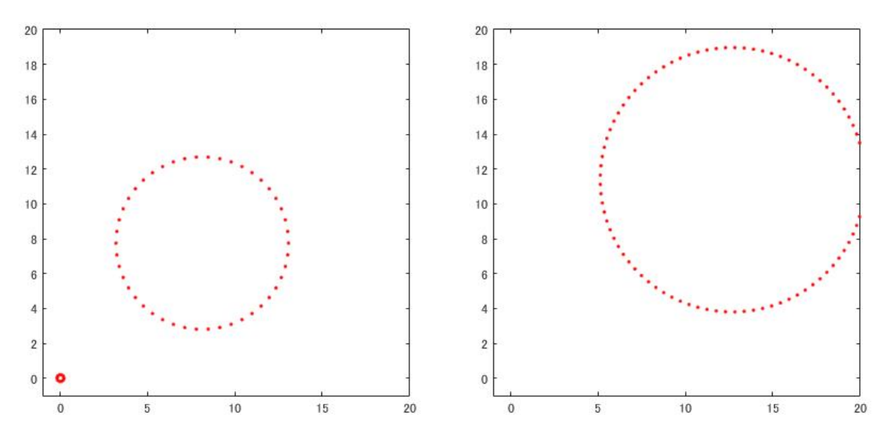
For the binary classification, we introduce the following labels:
| if a generator for is born before and dies after . | |||
| if exists. |
The class label of the data set is then given by . By this construction, identifying requires relatively smooth function in the area of long lifetimes, while classifying the existing of needs delicate control of the resolution around the diagonal.
4.2.2 SVM results
SVMs are trained from persistence diagrams given by 100 data sets, and evaluated with 100 independent test data sets. As a positive definite kernel , we choose the Gaussian kernel and the linear kernel . For a weight function , we use the proposed function , the piecewise linear weighting function defined in Section 4.1.3, and an unweighted function . The hyper-parameters in the PWGK and in the PSSK are chosen by the 10-fold cross-validation, and the degree in is set as . For and , while they originally consider only the inner product, we also apply the Gaussian kernels on RKHS following Equation (11). Since can be seen as a discretization of the -linear kernel, we also construct another kernel of persistence image by replacing with , which is considered as a discretization of the PWGK. In order to check whether the persistence image with is an appropriate discretization of the PWGK, we try several mesh size .
| Linear | Gaussian | ||
| PWGK | |||
| kernel | weight | ||
| 75.7 2.31 | 85.8 5.19 (PWGK) | ||
| 75.8 2.47 () | 85.6 5.01 (PWGK, ) | ||
| 76.0 2.39 | 86.0 4.98 (PWGK) | ||
| 49.3 2.72 | 52.3 6.60 | ||
| 53.8 4.76 | 55.1 8.42 | ||
| 49.3 6.92 | 51.8 3.52 | ||
| 51.0 6.84 | 55.7 8.68 | ||
| 50.5 6.90 | 53.0 4.89 | ||
| PWGK with Persistence image | |||
| 48.8 3.75 () | 52.0 5.65 () | ||
| 49.2 5.77 () | 51.8 7.23 () | ||
| 75.0 2.20 () | 85.8 4.15 () | ||
| PSSK | 50.5 5.60 () | 53.6 6.69 | |
| Persistence landscape | 50.6 5.92 () | 48.8 4.25 | |
| Persistence image | |||
| 51.1 4.38 ) | 51.7 6.86 | ||
| 49.0 6.14 ) | 52.3 7.21 | ||
| 54.5 8.76 ) | 52.1 6.70 | ||
In Table 1, we can see that the PWGK and the Gaussian kernel on the persistence image with and large mesh size show higher classification rates ( accuracy) than the other methods (, , and ). Although the -Gaussian kernel and the persistence image with the original weight discount noisy generators, the classification rates are close the chance level. These unfavorable results must be caused by the difficulty in handling the local and global locations of generators simultaneously. While the result of the persistence image with a large mesh size is similar to that of the PWGK (e.g., and ), a small mesh size gives bad approximation results (e.g., and ). The reason is because a small mesh size makes rough pixels, and itself and noisy generators are treated in some rough pixel. On the other hand, we remark that a large mesh size needs much computational time since the computational complexity of the persistence image depends on .
We observe that the classification accuracies are not sensitive to . Thus, in the rest of this paper, we set because the assumption in Theorem 3.3 ensures the continuity in the kernel embedding of persistence diagrams and all data points are obtained from .
4.3 Analysis of granular system
We apply the PWGK, the PSSK, the persistence landscape, and the persistence image to persistence diagrams obtained by experimental data in a granular packing system [FSCS13]. In this example, a partially crystallized packing with monosized beads (diameter mm, polydispersity mm) in a container is obtained by experiments, where the configuration of the beads is imaged by means of X-ray Computed Tomography. One of the fundamental interests in the study of granular packings is to understand the transition from random packings to crystallized packings. In particular, the maximum packing density that random packings can attain is still a controversial issue (e.g., see [TTD00]). Here, we apply the change point analysis to detect .
In oder to observe configurations of various densities, we divide the original full system into cubical subsets containing approximately beads. The data are provided by the authors of the paper [FSCS13]. The packing densities of the subsets range from to . [STR+17] computed a persistence diagram for each subset by taking the beads configuration as a finite subset in , and found that the persistence diagrams characterize different configurations in random packings (small ) and crystallized packings (large ). Hence, it is expected that the change point analysis applied to these persistence diagrams can detect the maximum packing density as a transition from the random to crystallized packings.
Our strategy is to regard the maximum packing density as the change point and detect it from a collection of persistence diagrams made by beads configurations of granular systems, where is the index of the packing densities listed in the increasing order. As a statistical quantity for the change point detection, we use the kernel Fisher discriminant ratio [HMB09] defined by
| (18) |
where the empirical mean element and the empirical covariance operator with data through are given by
respectively, and is a regularization parameter (in this paper we set ). The index achieving the maximum of corresponds to the estimated change point. In Figure 8, all the four methods detect as the sharp maximizer of the KFDR. This result indicates that the maximum packing density exists in the interval and supports the traditional observation [Ano72].

We also apply kernel principal component analysis (KPCA) to the same collection of the 35 persistence diagrams. Figure 9 shows the -dimensional KPCA plots where each green triangle (resp. red circle) indicates the persistence diagram of random packing (resp. crystallized packing). We can see clear two-cluster structure corresponding to two physical states.

4.4 Analysis of
When we rapidly cool down the liquid state of , it avoids the usual crystallization and changes into a glass state. Understanding the liquid-glass transition is an important issue for the current physics and industrial applications [GS07]. Glass is an amorphous solid, which does not have a clear structure in the configuration of molecules, but it is also known that the medium distance structure such as rings have important influence on the physical properties of the material. It is thus promising to apply the persistent homology to express the topological and geometrical structure of the glass configuration. For estimating the glass transition temperature by simulations, a traditional physical method is to prepare atomic configurations of for a certain range of temperatures by molecular dynamics simulations, and then draw the temperature-enthalpy graph. The graph consists of two lines in high and low temperatures with slightly different slopes which correspond to the liquid and the glass states, respectively, and the glass transition temperature is conventionally estimated as an interval of the transient region combining these two lines (e.g., see [Ell90]). However, since the slopes of two lines are close to each other, determining the interval is a subtle problem. Usually only the rough estimate of the interval is available. Hence, we apply our framework of topological data analysis with kernels to detect the glass transition temperature.
Let be a collection of the persistence diagrams made by atomic configurations of and sorted by the decreasing order of the temperature. The same data was used in the previous works by [HNH+16, NHH+15]. The interval of the glass transition temperature estimated by the conventional method explained above is , which corresponds to .
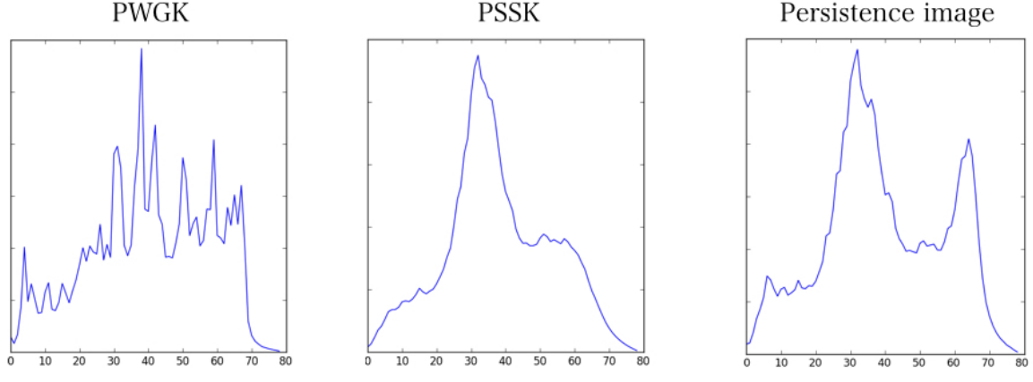
In Figure 10, the KFDR plots show that the change point is estimated as by the PWGK, by the PSSK, and by the persistence image. For the persistence landscape, we cannot obtain the KFDR or the KPCA results with reasonable computational time.
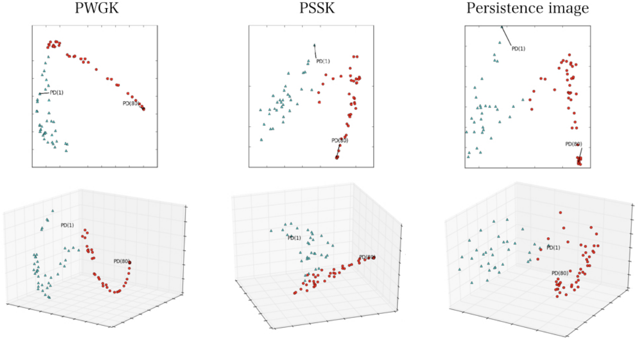
As we see from the -dimensional plots given by KPCA (Figure 11), the PWGK presents the clear phase change between before (green triangle) and after (red circle) the change point determined by the KFDR. This strongly suggests that the glass transition occurs at the detected change point. On the other hand, we cannot observe clear two-cluster structure in the KPCA plots of the PSSK and the persistence image. We also remark that the detailed cluster structure is observed in the -dimensional KPCA plots of the PWGK.
4.5 Protein classification
We apply the PWGK to two classification tasks studied in [CMW+15]. They introduced the molecular topological fingerprint (MTF) as a feature vector constructed from the persistent homology, and used it for the input to the SVM. The MTF is given by the -dimensional vector whose elements consist of the persistences of some specific generators1414 14 The MTF method is not a general method for persistence diagrams because some elements of the MTF vector are specialized for protein data, e.g., the ninth element of the MTF vector is defined by the number of Betti bars that locate at Å, divided by the number of atoms. For the details, see [CMW+15]. in persistence diagrams. We compare the performance between the PWGK and the MTF method under the same setting of the SVM reported in [CMW+15].
The first task is a protein-drug binding problem, where the binding and non-binding of drug to the M2 channel protein of the influenza A virus is to be classified. For each of the two forms, 15 data were obtained by NMR experiments, and 10 data are used for training and the remaining for testing. We randomly generate 100 ways of partitions and calculate the average classification rates.
In the second problem, the taut and relaxed forms of hemoglobin are to be classified. For each form, 9 data were collected by the X-ray crystallography. We select one data from each class for testing and use the remaining for training. All the 81 combinations are performed to calculate the CV classification rates.
The results of the two problems are shown in Table 2. We can see that the PWGK achieves better performance than the MTF in both problems.
| Protein-Drug | Hemoglobin | |
|---|---|---|
| PWGK | 100 | 88.90 |
| MTF | (nbd) 93.91 / (bd) 98.31 | 84.50 |
5 Conclusion and Discussions
One of the contributions of this paper is to introduce a kernel framework to topological data analysis with persistence diagrams. We applied the kernel embedding approach to vectorize the persistence diagrams, which enables us to utilize any standard kernel methods for data analysis. Another contribution is to propose a kernel specific to persistence diagrams, that is called persistence weighted Gaussian kernel (PWGK). As a significant advantage, our kernel enables one to control the effect of persistence in data analysis. We have also proven the stability property with respect to the distance in the Hilbert space. Furthermore, we have analyzed the synthesized and real data by using the proposed kernel. The change point detection, the principal component analysis, and the support vector machine derived meaningful results for the tasks. From the viewpoint of computations, our kernel can utilize an efficient approximation to compute the Gram matrix.
One of the main theoretical results of this paper is the stability of the PWGK (Theorem 3.3). It is obtained as a corollary of Proposition 3.2 by restricting the class of persistence diagrams to that obtained from ball model filtrations. The reason of this restriction is because the total persistence can be bounded from above independent of the persistence diagram. Thus, one direction to extend this work is to examine the boundedness condition about the total persistence of other persistence diagrams, for example obtained from sub-level sets or Rips complexes.
Another direction to extend this work is to generalize the class of weight functions. The reason of the choice of is mainly for the stability property, but in principle, we can apply any weight function to data analysis. Then, the question is what types of weight functions have a stability property with respect to the bottleneck or -Wasserstein distance. Even if we do not concern about stability properties, which weight function is practically good for data analysis? Suppose generators close to the diagonal are sometimes seen as important features. Then, our statistical framework can treat such small generators as significant ones by a weight function which has large weight close to the diagonal, while other statistical methods for persistence diagrams always see small generators as noisy ones.
Acknowledgement
We thank Ulrich Bauer for giving us useful comments in Section 4.1.1, and Mohammad Saadatfar and Takenobu Nakamura for providing experimental and simulation data used in Section 4.3 and 4.4. This work is partially supported by JST CREST Mathematics (15656429), JSPS KAKENHI Grant Number 26540016, Structural Materials for Innovation Strategic Innovation Promotion Program D72, Materials research by Information Integration” Initiative (MI2I) project of the Support Program for Starting Up, Innovation Hub from JST, and JSPS Research Fellow (17J02401).
Appendix A Topological tools
This section summarizes some topological tools used in the paper. To study topological properties algebraically, simplicial complexes are often considered as basic objects. We start with a brief explanation of simplicial complexes, and gradually increase the generality from simplicial homology to singular and persistent homology. For more details, see [Hat02].
A.1 Simplicial complex
We first introduce a combinatorial geometric model called simplicial complex to define homology. Let be a finite set (not necessarily points in a metric space). A simplicial complex with the vertex set is defined by a collection of subsets in satisfying the following properties:
- 1.
for , and
- 2.
if and , then .
Each subset with vertices is called a -simplex. We denote the set of -simplices by . A subcollection which also becomes a simplicial complex (with possibly less vertices) is called a subcomplex of .
We can visually deal with a simplicial complex as a polyhedron by pasting simplices in into a Euclidean space. The simplicial complex obtained in this way is called a geometric realization, and its polyhedron is denoted by . In this context, the simplices with small correspond to points (), edges (), triangles (), and tetrahedra ().
Example A.1.
Figure 12 shows two polyhedra of simplicial complexes
A.2 Homology
A.2.1 Simplicial homology
The procedure to define homology is summarized as follows:
- 1.
Given a simplicial complex , build a chain complex . This is an algebraization of characterizing the boundary.
- 2.
Define homology by quotienting out certain subspaces in characterized by the boundary.
We begin with the procedure 1 by assigning orderings on simplices. When we deal with a -simplex as an ordered set, there are orderings on . For , we define an equivalence relation on two orderings of such that they are mapped to each other by even permutations. By definition, two equivalence classes exist, and each of them is called an oriented simplex. An oriented simplex is denoted by , and its opposite orientation is expressed by adding the minus . We write for the equivalence class including . For , we suppose that we have only one orientation for each vertex.
Let be a field. We construct a -vector space as
for and for . Here, for a set is a vector space over such that the elements of formally form a basis of the vector space. Furthermore, we define a linear map called the boundary map by the linear extension of
| (19) |
where means the removal of the vertex . We can regard the linear map as algebraically capturing the -dimensional boundary of a -dimensional object.
For example, the image of the -simplex is given by , which is the boundary of (see Figure 12).
In practice, by arranging some orderings of the oriented - and - simplices, we can represent the boundary map as a matrix with the entry given by the coefficient in (19). For the simplicial complex in Example A.1, the matrix representations and of the boundary maps are given by
Here, the -simplices (resp. -simplices) are ordered by (resp. , , ).
We call a sequence of the vector spaces and linear maps
the chain complex of . As an easy exercise, we can show . Hence, the subspaces and satisfy . Then, the -th (simplicial) homology is defined by taking the quotient space
Intuitively, the dimension of counts the number of -dimensional holes in and each generator of the vector space corresponds to these holes. We remark that the homology as a vector space is independent of the orientations of simplices.
For a subcomplex of , the inclusion map naturally induces a linear map in homology . Namely, an element is mapped to , where the equivalence class is taken in each vector space.
For example, the simplicial complex in Example A.1 has
from (A.2.1). Hence , meaning that there are no -dimensional hole (ring) in . On the other hand, since and , we have , meaning that consists of one ring. Hence, the induced linear map means that the ring in disappears in under .
A topological space is called triangulable if there exists a geometric realization of a simplicial complex whose polyhedron is homeomorphic1515 15 A continuous map is said to be homeomorphic if is bijective and the inverse is also continuous. to . For such a triangulable topological space, the homology is defined by . This is well-defined, since a different geometric realization provides an isomorphic homology.
A.2.2 Singular homology
We here extend the homology to general topological spaces. Let be the standard basis of (i.e., , 1 at -th position, and 0 otherwise), and set
We also denote the inclusion by .
For a topological space , a continuous map is called a singular -simplex, and let be the set of -simplices. We construct a -vector space as
The boundary map is defined by the linear extension of
Even in this setting, we can show that , and hence the subspaces and satisfy . Then, the -th (singular) homology is similarly defined by
It is known that, for a triangulable topological space, the homology of this definition is isomorphic to that defined in A.2.1. From this reason, we hereafter identify simplicial and singular homology.
The induced linear map in homology for an inclusion pair of topological space is similarly defined as in A.2.1.
Appendix B Total persistence
Let be a triangulable compact metric space. For a Lipschitz function , we define the degree- total persistence over by
for , where is the amplitude of . Let be a triangulated simplicial complex of by a homeomorphism . The diameter of a simplex and the mesh of the triangulation are defined by and , respectively. Furthermore, let us set . Then, the degree- total persistence over is bounded from above as follows:
Lemma B.1 ([CSEHM10]).
Let be a triangulable compact metric space and be a tame Lipschitz function. Then, is bounded from above by
where is the Lipschitz constant of .
For a compact triangulable subspace in , the number of -cubes with length covering is bounded from above by , and hence there exists some constant depending only on such that .
For , we can find the upper bounds for the both terms as follows:
and
Then, the upper bound of the total persistence is given as follows:
Lemma B.2.
Let be a triangulable compact subspace in and . For any Lipschitz function ,
where is a constant depending only on .
In the case of a finite subset , there always exists an -ball containing for some , which is a triangulable compact subspace in . Moreover, by estimating , we show Lemma 2.4 as a corollary of Lemma B.2:
Lemma 2.4.
The Lipschitz constant of is , because, for any ,
Moreover,
because and . Thus, for some constant depending only on , we have
∎
For a persistence diagram , we construct a -dimensional vector
Then, the degree- total persistence is represented as
where denotes the -norm of . Since , we have
Proposition B.3.
If and is bounded from above, is also bounded from above.
Appendix C Lemmata for Proposition 3.2
Lemma C.1.
For any , .
Lemma C.2.
For any , the difference of persistences is less than or equal to .
Proof.
For , we have
∎
Lemma C.3.
For any , we have
Appendix D Remark on the bottleneck stability of the PWGK
Let be a positive definite kernel on persistence diagrams. Then,
defines a semi-metric on persistence diagrams. A positive definite kernel is said to be additive if and trivial if for any persistence diagrams . It is shown that a non-trivial additive kernel does not satisfy the stability for by giving a counterexample.
Proposition D.1 ([RHBK15]).
Let be a non-trivial additive positive definite kernel on persistence diagrams such that for the diagonal set . Then, for any , there exists no constant such that
Proof.
Since is non-trivial, there exists a persistence diagram such that . Then, for any , we compute both distance between and the diagonal set :
Hence, cannot be bounded by with a constant . ∎
Actually, since the kernel defined by is non-trivial, additive, and , it seems that the PWGK would not satisfy the bottleneck stability and it contradicts Theorem 3.3. However, when this counterexample is applied to Proposition 3.2, because and , we obtain
In other words, Proposition 3.2 is not affected by in and Theorem 3.3 does not contradict with Proposition D.1.
References
- [AEK+17] Henry Adams, Tegan Emerson, Michael Kirby, Rachel Neville, Chris Peterson, Patrick Shipman, Sofya Chepushtanova, Eric Hanson, Francis Motta, and Lori Ziegelmeier. Persistence images: A stable vector representation of persistent homology. Journal of Machine Learning Research, 18(8):1–35, 2017.
- [Ano72] Anonymous. What is random packing? Nature, 239:488–489, 1972.
- [BD17] Peter Bubenik and Paweł Dłotko. A persistence landscapes toolbox for topological statistics. Journal of Symbolic Computation, 78:91–114, 2017.
- [BKRW14] Ulrich Bauer, Michael Kerber, Jan Reininghaus, and Hubert Wagner. Mathematical Software – ICMS 2014: 4th International Congress, Seoul, South Korea, August 5-9, 2014. Proceedings, chapter PHAT – Persistent Homology Algorithms Toolbox, pages 137–143. Springer Berlin Heidelberg, Berlin, Heidelberg, 2014.
- [Bub15] Peter Bubenik. Statistical topological data analysis using persistence landscapes. Journal of Machine Learning Research, 16(1):77–102, 2015.
- [Car09] Gunnar Carlsson. Topology and data. Bulletin of the American Mathematical Society, 46(2):255–308, 2009.
- [CdSO14] Frédéric Chazal, Vin de Silva, and Steve Oudot. Persistence stability for geometric complexes. Geometriae Dedicata, 173(1):193–214, 2014.
- [CGLM15] Frédéric Chazal, Marc Glisse, Catherine Labruère, and Bertrand Michel. Convergence rates for persistence diagram estimation in topological data analysis. Journal of Machine Learning Research, 16:3603–3635, 2015.
- [CIdSZ08] Gunnar Carlsson, Tigran Ishkhanov, Vin de Silva, and Afra Zomorodian. On the local behavior of spaces of natural images. International journal of computer vision, 76(1):1–12, 2008.
- [CMW+15] Zixuan Cang, Lin Mu, Kedi Wu, Kristopher Opron, Kelin Xia, and Guo-Wei Wei. A topological approach for protein classification. Molecular Based Mathematical Biology, 3(1), 2015.
- [COO15] Mathieu Carrière, Steve Oudot, and Maks Ovsjanikov. Local signatures using persistence diagrams. preprint, 2015.
- [CSEH07] David Cohen-Steiner, Herbert Edelsbrunner, and John Harer. Stability of persistence diagrams. Discrete & Computational Geometry, 37(1):103–120, 2007.
- [CSEHM10] David Cohen-Steiner, Herbert Edelsbrunner, John Harer, and Yuriy Mileyko. Lipschitz functions have -stable persistence. Foundations of computational mathematics, 10(2):127–139, 2010.
- [DLY15] Tran Kai Frank Da, Sébastien Loriot, and Mariette Yvinec. 3D alpha shapes. In CGAL User and Reference Manual. CGAL Editorial Board, 4.7 edition, 2015.
- [dSG07] Vin de Silva and Robert Ghrist. Coverage in sensor networks via persistent homology. Algebraic & Geometric Topology, 7(1):339–358, 2007.
- [DUJ77] Joseph Diestel and J Jerry Uhl Jr. Vector measures. with a foreword by bj pettis. mathematical surveys, no. 15. American Mathematical Society, Providence, RI, 56:12216, 1977.
- [Ell90] Stephen R. Elliott. Physics of amorphous materials (2nd). Longman London; New York, 1990.
- [ELZ02] Herbert Edelsbrunner, David Letscher, and Afra Zomorodian. Topological persistence and simplification. Discrete and Computational Geometry, 28(4):511–533, 2002.
- [FLR+14] Brittany Terese Fasy, Fabrizio Lecci, Alessandro Rinaldo, Larry Wasserman, Sivaraman Balakrishnan, and Aarti Singh. Confidence sets for persistence diagrams. The Annals of Statistics, 42(6):2301–2339, 2014.
- [FSCS13] Nicolas Francois, Mohammad Saadatfar, R Cruikshank, and A Sheppard. Geometrical frustration in amorphous and partially crystallized packings of spheres. Physical review letters, 111(14):148001, 2013.
- [GFT+07] Arthur Gretton, Kenji Fukumizu, Choon H. Teo, Le Song, Bernhard Schölkopf, and Alex J Smola. A kernel statistical test of independence. In Advances in Neural Information Processing Systems, pages 585–592, 2007.
- [GHI+15] Marcio Gameiro, Yasuaki Hiraoka, Shunsuke Izumi, Miroslav Kramar, Konstantin Mischaikow, and Vidit Nanda. A topological measurement of protein compressibility. Japan Journal of Industrial and Applied Mathematics, 32(1):1–17, 2015.
- [GS07] Neville G Greaves and Sabyasachi Sen. Inorganic glasses, glass-forming liquids and amorphizing solids. Advances in Physics, 56(1):1–166, 2007.
- [Hat02] Allen Hatcher. Algebraic topology. Cambridge University Press, 2002.
- [HMB09] Zaid Harchaoui, Eric Moulines, and Francis R. Bach. Kernel change-point analysis. In Advances in Neural Information Processing Systems, pages 609–616, 2009.
- [HNH+16] Yasuaki Hiraoka, Takenobu Nakamura, Akihiko Hirata, Emerson G Escolar, Kaname Matsue, and Yasumasa Nishiura. Hierarchical structures of amorphous solids characterized by persistent homology. Proceedings of the National Academy of Sciences, 113(26):7035–7040, 2016.
- [KHF16] Genki Kusano, Yasuaki Hiraoka, and Kenji Fukumizu. Persistence weighted gaussian kernel for topological data analysis. In International Conference on Machine Learning, pages 2004–2013, 2016.
- [KZP+07] Peter M Kasson, Afra Zomorodian, Sanghyun Park, Nina Singhal, Leonidas J Guibas, and Vijay S Pande. Persistent voids: a new structural metric for membrane fusion. Bioinformatics, 23(14):1753–1759, 2007.
- [LCK+11] Hyekyoung Lee, Moo K Chung, Hyejin Kang, Bung-Nyun Kim, and Dong Soo Lee. Discriminative persistent homology of brain networks. In Biomedical Imaging: From Nano to Macro, 2011 IEEE International Symposium on, pages 841–844. IEEE, 2011.
- [MFDS12] Krikamol Muandet, Kenji Fukumizu, Francesco Dinuzzo, and Bernhard Schölkopf. Learning from distributions via support measure machines. In Advances in neural information processing systems, pages 10–18, 2012.
- [MFSSar] Krikamol Muandet, Kenji Fukumizu, Bharath K. Sriperumbudur, and Bernhard Schölkopf. Kernel mean embedding of distributions: A review and beyonds. Foundations and Trends in Machine Learning, To appear.
- [NHH+15] Takenobu Nakamura, Yasuaki Hiraoka, Akihiko Hirata, Emerson G Escolar, and Yasumasa Nishiura. Persistent homology and many-body atomic structure for medium-range order in the glass. Nanotechnology, 26(304001), 2015.
- [PET+14] Giovanni Petri, Paul Expert, Federico Turkheimer, Robin Carhart-Harris, David Nutt, Peter J Hellyer, and Francesco Vaccarino. Homological scaffolds of brain functional networks. Journal of The Royal Society Interface, 11(101):20140873, 2014.
- [RHBK15] Jan Reininghaus, Stefan Huber, Ulrich Bauer, and Roland Kwitt. A stable multi-scale kernel for topological machine learning. In In Proceedings of the IEEE Conference on Computer Vision and Pattern Recognition(CVPR), pages 4741–4748, 2015.
- [RR07] Ali Rahimi and Benjamin Recht. Random features for large-scale kernel machines. In Advances in neural information processing systems, pages 1177–1184, 2007.
- [RT16] Vanessa Robins and Katharine Turner. Principal component analysis of persistent homology rank functions with case studies of spatial point patterns, sphere packing and colloids. Physica D: Nonlinear Phenomena, 334:99–117, 2016.
- [SFG13] Le Song, Kenji Fukumizu, and Arthur Gretton. Kernel embeddings of conditional distributions: A unified kernel framework for nonparametric inference in graphical models. IEEE Signal Processing Magazine, 30(4):98–111, 2013.
- [SFL11] Bharath K. Sriperumbudur, Kenji Fukumizu, and Gert R. G. Lanckriet. Universality, characteristic kernels and rkhs embedding of measures. The Journal of Machine Learning Research, 12:2389–2410, 2011.
- [SGSS07] Alex Smola, Arthur Gretton, Le Song, and Bernhard Schölkopf. A hilbert space embedding for distributions. In In Algorithmic Learning Theory: 18th International Conference, pages 13–31. Springer, 2007.
- [SMI+08] Gurjeet Singh, Facundo Memoli, Tigran Ishkhanov, Guillermo Sapiro, Gunnar Carlsson, and Dario L Ringach. Topological analysis of population activity in visual cortex. Journal of vision, 8(8):11, 2008.
- [STR+17] Mohammad Saadatfar, Hiroshi Takeuchi, Vanessa Robins, Nicolas Francois, and Yasuaki Hiraoka. Pore configuration landscape of granular crystallization. Nature Communications, 8:15082 EP, 2017.
- [TTD00] Salvatore Torquato, Thomas M Truskett, and Pablo G Debenedetti. Is random close packing of spheres well defined? Physical review letters, 84(10):2064, 2000.
- [XW14] Kelin Xia and Guo-Wei Wei. Persistent homology analysis of protein structure, flexibility, and folding. International journal for numerical methods in biomedical engineering, 30(8):814–844, 2014.
- [ZC05] Afra Zomorodian and Gunnar Carlsson. Computing persistent homology. Discrete & Computational Geometry, 33(2):249–274, 2005.