Sliced Wasserstein Kernel for Persistence Diagrams

Mathieu Carrière Marco Cuturi Steve Oudot

Abstract

Persistence diagrams play a key role in topological data analysis (TDA), in which they are routinely used to describe topological properties of complicated shapes. persistence diagrams enjoy strong stability properties and have proven their utility in various learning contexts. They do not, however, live in a space naturally endowed with a Hilbert structure and are usually compared with non-Hilbertian distances, such as the bottleneck distance. To incorporate persistence diagrams in a convex learning pipeline, several kernels have been proposed with a strong emphasis on the stability of the resulting RKHS distance w.r.t. perturbations of the persistence diagrams. In this article, we use the Sliced Wasserstein approximation of the Wasserstein distance to define a new kernel for persistence diagrams, which is not only provably stable but also discriminative (with a bound depending on the number of points in the persistence diagrams) w.r.t. the first diagram distance between persistence diagrams. We also demonstrate its practicality, by developing an approximation technique to reduce kernel computation time, and show that our proposal compares favorably to existing kernels for persistence diagrams on several benchmarks.

1 Introduction

Topological Data Analysis (TDA) is an emerging trend in data science, grounded on topological methods to design descriptors for complex data—see e.g. [5] for an introduction to the subject. The descriptors of TDA can be used in various contexts, in particular statistical learning and geometric inference, where they provide useful insight into the structure of data. Applications of TDA can be found in a number of scientific areas, including computer vision [26], materials science [20], and brain science [37], to name a few. The tools developed in TDA are built upon persistent homology theory [15, 29], and their main output is a descriptor called persistence diagram, which encodes the topology of a space at all scales in the form of a point cloud with multiplicities in the plane $\mathbb{R}^{2}$ —see Section 2.1 for more details.

Persistence diagrams as features.

The main strength of persistence diagrams is their stability with respect to perturbations of the data [9, 11]. On the downside, their use in learning tasks is not straightforward. Indeed, a large class of learning methods, such as SVM or PCA, requires a Hilbert structure on the descriptors space, which is not the case for the space of persistence diagrams. Actually, many simple operators of $\mathbb{R}^{n}$ , such as addition, average or scalar product, have no analogues in that space. Mapping persistence diagrams to vectors in $\mathbb{R}^{n}$ or in some infinite-dimensional Hilbert space is one possible approach to facilitate their use in discriminative settings.

Related work.

A series of recent contributions have proposed kernels for persistence diagrams, falling into two classes. The first class of methods builds explicit feature maps: one can, for instance, compute and sample functions extracted from persistence diagrams [4, 1, 35]; sort the entries of the distance matrices of the persistence diagrams [6]; treat the points of the persistence diagrams as roots of a complex polynomial, whose coefficients are concatenated [14]. The second class of methods, which is more relevant to our work, defines implicitly feature maps by focusing instead on building kernels for persistence diagrams. For instance, [34] use solutions of the heat differential equation in the plane and compare them with the usual $L^{2}(\mathbb{R}^{2})$ dot product. [23] handle a persistence diagram as a discrete measure on the plane, and follow by using kernel mean embeddings with Gaussian kernels—see Section 4 for precise definitions. Both kernels are provably stable, in the sense that the metric they induce in their respective reproducing kernel Hilbert space (RKHS) is bounded above by the distance between persistence diagrams. Although these kernels are injective, there is no evidence that their induced RKHS distances are discriminative and therefore follow the geometry of the diagram distances, which are more widely accepted distances to compare persistence diagrams.

More generally, one of the reasons why the derivation of kernels for persistence diagrams is not straightforward is that the natural metrics between persistence diagrams, the diagram distances are not negative semi-definite. Indeed, these diagram distances are very similar to the Wasserstein distance [41, §6] between probability measures, which is not negative semi-definite. However, a relaxation of this metric called the Sliced Wasserstein distance [31] has recently been shown to be negative semi-definite and was used to derive kernels for probability distributions in [21].

Contributions.

In this article, we use the Sliced Wasserstein distance of [31] to define a new kernel for persistence diagrams, which we prove to be both stable and discriminative. Specifically, we provide distortion bounds on the Sliced Wasserstein distance that quantify its ability to mimic the diagram distances between persistence diagrams. This is in contrast to other kernels for persistence diagrams, which only focus on stability. We also propose a simple approximation algorithm to speed up the computation of that kernel, confirm experimentally its discriminative power and show that it outperforms experimentally both proposals of [23] and [34] in several supervised classification problems.

2 Background

2.1 Persistent Homology

Refer to caption — Figure 1: Sketch of persistent homology: (a) the horizontal lines are the boundaries of sublevel sets $f((-\infty,t])$ , which are colored in decreasing shades of grey. The vertical dotted lines are the boundaries of their different connected components. For instance, a new connected component is created in the sublevel set $f^{-1}((-\infty,t])$ when $t=f(p)$ , and it is merged (destroyed) when $t=f(s)$ ; its lifespan is represented by a copy of the point with coordinates $(f(p),f(s))$ in the persistence diagram of $f$ (Figure (c)); (b) a piecewise-linear approximation $g$ (blue) of the function $f$ (red) from sampled values; (c) superposition of $\mathrm{Dg}(f)$ (red) and $\mathrm{Dg}(g)$ (blue), showing the partial matching of minimum cost (magenta) between the two persistence diagrams.

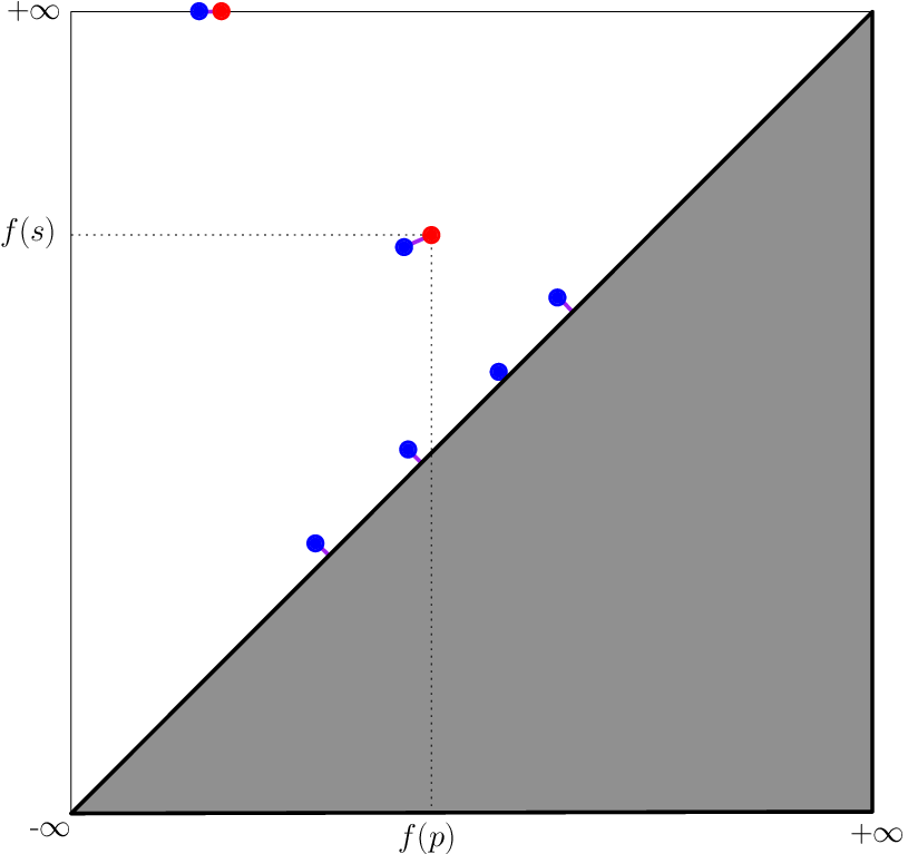
Persistent homology is a technique inherited from algebraic topology for computing stable descriptors on real-valued functions. Given $f:X\to\mathbb{R}$ as input, persistent homology outputs a planar point set with multiplicities, called the persistence diagram of $f$ and denoted by $\mathrm{Dg}(f)$ . Note that the coordinates of the points belong to the extended real line $\mathbb{R}_{\text{ext}}=\mathbb{R}\cup\{+\infty\}$ . See Figure 1 for an example. To understand the meaning of each point in this diagram, it suffices to know that, to compute $\mathrm{Dg}(f)$ , persistent homology considers the family of sublevel sets of $f$ , i.e. the sets of the form $f^{-1}((-\infty,t])$ for $t\in\mathbb{R}$ , and it records the topological events (e.g. creation or merge of a connected component, creation or filling of a loop, void, etc.) that occur in $f^{-1}((-\infty,t])$ as $t$ ranges from $-\infty$ to $+\infty$ . Then, each point $p\in\mathrm{Dg}(f)$ represents the lifespan of a particular topological feature (connected component, loop, void, etc.), with its creation and destruction times as coordinates. See again Figure 1 for an illustration.

For the interested reader, we point out that the mathematical tool used by persistent homology to track the topological events in the family of sublevel sets is homological algebra, which turns the parametrized family of sublevel sets into a parametrized family of vector spaces and linear maps. Computing persistent homology then boils down to computing a family of bases for the vector spaces, which are compatible with the linear maps. It will be no surprise to the reader familiar with matrix reduction techniques that the simplest way to implement the compatible basis computation is using Gaussian elimination.

Distance between persistence diagrams.

We now define the $p$ th diagram distance between persistence diagrams. Let $p\in\mathbb{N}$ and $\mathrm{Dg}_{1},\mathrm{Dg}_{2}$ be two persistence diagrams. Let $\Gamma:\mathrm{Dg}_{1}\supseteq A\rightarrow B\subseteq\mathrm{Dg}_{2}$ be a partial bijection between $\mathrm{Dg}_{1}$ and $\mathrm{Dg}_{2}$ . Then, for any point $x\in A$ , the $p$ -cost of $x$ is defined as $c_{p}(x)=\|x-\Gamma(x)\|_{\infty}^{p}$ , and for any point $y\in(\mathrm{Dg}_{1}\sqcup\mathrm{Dg}_{2})\setminus(A\sqcup B)$ , the $p$ -cost of $y$ is defined as $c^{\prime}_{p}(y)=\|y-\pi_{\Delta}(y)\|_{\infty}^{p}$ , where $\pi_{\Delta}$ is the projection onto the diagonal $\Delta=\{(x,x):x\in\mathbb{R}\}$ . The cost $\operatorname{c}_{p}(\Gamma)$ is defined as: $\operatorname{c}_{p}(\Gamma)=(\sum_{x}c_{p}(x)+\sum_{y}c^{\prime}_{p}(y))^{1/p}.$ We then define the $p$ th diagram distance $d_{p}$ as the cost of the best partial bijection:

d_{p}(\mathrm{Dg}_{1},\mathrm{Dg}_{2})=\inf_{\Gamma}\operatorname{c}_{p}(\Gamma).

In the particular case $p=+\infty$ , the cost of $\Gamma$ is defined as $\operatorname{c}(\Gamma)=\max\{\max_{x}c_{1}(x)+\max_{y}c^{\prime}_{1}(y)\}.$ The corresponding distance $d_{\infty}$ is often called the bottleneck distance. One can show that $d_{p}\rightarrow d_{\infty}$ when $p\rightarrow+\infty$ . A fundamental property of persistence diagrams is their stability with respect to (small) perturbations of their originating functions. Indeed, the stability theorem [2, 8, 10, 13] asserts that for any $f,g:X\to\mathbb{R}$ , we have

d_{\infty}(\mathrm{Dg}(f),\,\mathrm{Dg}(g))\leq\|f-g\|_{\infty},

(1)

In practice, persistence diagrams can be used as descriptors for data via the choice of appropriate filtering functions $f$ , e.g. distance to the data in the ambient space, eccentricity, curvature, etc. The main strengths of the obtained descriptors are: (a) to be provably stable as mentioned previously; (b) to be invariant under reparametrization of the data; and (c) to encode information about the topology of the data, which is complementary and of an essentially different nature compared to geometric or statistical quantities. These properties have made persistence diagrams useful in a variety of contexts, including the ones mentioned in the introduction of the paper. For further details on persistent homology and on applications of persistence diagrams, the interested reader can refer e.g. to [29] and the references therein.

Notation.

Let ${\mathcal{D}}$ be the space of persistence diagrams with at most countably many points, ${\mathcal{D}}_{\rm f}^{\rm b}$ be the space of finite and bounded persistence diagrams, and ${\mathcal{D}}_{N}^{\rm b}$ be the space of bounded persistence diagrams with less than $N$ points. Obviously, we have the following sequence of (strict) inclusions: ${\mathcal{D}}_{N}^{\rm b}\subset{\mathcal{D}}_{\rm f}^{\rm b}\subset{\mathcal{D}}$ .

2.2 Kernel Methods

Positive Definite Kernels. Given a set $X$ , a function $k:X\times X\to\mathbb{R}$ is called a positive definite kernel if for all integers $n$ , for all families $x_{1},\cdots,x_{n}$ of points in $X$ , the matrix $[k(x_{i},x_{j})]_{i,j}$ is itself positive semi-definite. For brevity we will refer to positive definite kernels as kernels in the rest of the paper. It is known that kernels generalize scalar products, in the sense that, given a kernel $k$ , there exists a Reproducing Kernel Hilbert Space (RKHS) $\mathcal{H}_{k}$ and a feature map $\phi:X\to\mathcal{H}_{k}$ such that $k(x_{1},x_{2})=\langle\phi(x_{1}),\phi(x_{2})\rangle_{\mathcal{H}_{k}}$ . A kernel $k$ also induces a distance $d_{k}$ on $X$ that can be computed as the Hilbert norm of the difference between two embeddings:

d_{k}^{2}(x_{1},x_{2})\stackrel{{\scriptstyle\mbox{\tiny def.}}}{{=}}k(x_{1},x_{1})+k(x_{2},x_{2})-2\,k(x_{1},x_{2}).

We will be particularly interested in this distance, since one of the goals we will aim for will be that of designing a kernel $k$ for persistence diagrams such that $d_{k}$ has low distortion with respect to the first diagram distance $d_{1}$ .

Negative Definite and RBF Kernels.

A standard way to construct a kernel is to exponentiate the negative of a Euclidean distance. Indeed, the Gaussian kernel for vectors with parameter $\sigma>0$ does follow that template approach: $k_{\sigma}(x,y)={\rm exp}\left(-\frac{\|x-y\|^{2}}{2\sigma^{2}}\right)$ . An important theorem of [3] (Theorem 3.2.2, p.74) states that such an approach to build kernels, namely setting

k_{\sigma}(x,y)\stackrel{{\scriptstyle\mbox{\tiny def.}}}{{=}}{\rm exp}\left(-\frac{f(x,y)}{2\sigma^{2}}\right),

for an arbitrary function $f$ can only yield a valid positive definite kernel for all $\sigma>0$ if and only if $f$ is a conditionally negative definite function, namely that, for all integers $n$ , for all $x_{1},\cdots,x_{n}\in X$ , and for all $a_{1},\cdots,a_{n}\in\mathbb{R}$ such that $\sum_{i}a_{i}=0$ , one has $\sum_{i,j}a_{i}a_{j}f(x_{i},x_{j})\leq 0$ .

Unfortunately, as observed experimentally in Appendix A of [33], $d_{1}$ is not conditionally negative definite (in practice, it only suffices to sample a family of point clouds to observe experimentally that more often than not the inequality above will be violated for a particular weight vector $a$ ). Actually, as observed in [30], even the square of the diagram distances $d_{p}$ cannot be used to define Gaussian kernels. Indeed, it was noted in Theorem 6 of [16] that, if the square of a distance $d$ defined on a geodesic space $X$ is conditionally negative definite, then the metric space $X$ is flat, or CAT $(0)$ . However, since the metric space ${\mathcal{D}}$ , equipped with $d_{p}$ , $p\in\mathbb{N}\cup\{+\infty\}$ , is not CAT $(k)$ for any $k>0$ —which is due to the non-uniqueness of geodesics, see [40]—it follows that $d_{p}^{2}$ is not conditionally negative definite.

In this article, we use an approximation of $d_{1}$ with the Sliced Wasserstein distance, which is provably conditionally negative definite, and we use it to define a RBF kernel that can be easily tuned thanks to its bandwidth parameter $\sigma$ .

2.3 Wasserstein distance for unnormalized measures on $\mathbb{R}$

The Wasserstein distance [41, §6] is a distance between probability measures. For reasons that will become clear in the next section, we will focus on a variant of that distance: the 1-Wasserstein distance for nonnegative, not necessarily normalized, measures on the real line [36, §2]. Let $\mu$ and $\nu$ be two nonnegative measures on the real line such that $|\mu|=\mu(\mathbb{R})$ and $|\nu|=\nu(\mathbb{R})$ are equal to the same number $r$ . We define the three following objects:

		$\displaystyle\mathcal{W}(\mu,\nu)=\inf_{P\in\Pi(\mu,\nu)}\iint_{\mathbb{R}\times\mathbb{R}}\|x-y\|P({\rm d}x,{\rm d}y)$		(2)
		$\displaystyle\mathcal{Q}_{r}(\mu,\nu)=r\int_{\mathbb{R}}\|M^{-1}(x)-N^{-1}(x)\|{\rm d}x$		(3)
		$\displaystyle\mathcal{L}(\mu,\nu)=\inf_{f\in 1-\text{Lipschitz}}\int_{\mathbb{R}}f(x)[\mu({\rm d}x)-\nu({\rm d}x)]$		(4)

where $\Pi(\mu,\nu)$ is the set of measures on $\mathbb{R}^{2}$ with marginals $\mu$ and $\nu$ , and $M^{-1}$ and $N^{-1}$ the generalized quantile functions of the probability measures $\mu/r$ and $\nu/r$ respectively.

Proposition 2.1.

We have $\mathcal{W}=\mathcal{Q}_{r}=\mathcal{L}$ . Additionally (i) $\mathcal{Q}_{r}$ is conditionally negative definite on the space of measures of mass $r$ ; (ii) for any three positive measures $\mu,\nu,\gamma$ such that $|\mu|=|\nu|$ , we have $\mathcal{L}(\mu+\gamma,\nu+\gamma)=\mathcal{L}(\mu,\nu)$ .

Proof.

The equality between (2) and (3) is known for probability measures on the real line—see Proposition 2.17 in [36] for instance, and can be trivially generalized to unnormalized measures. The equality between (2) and (4) is due to the well known Kantorovich duality for a distance cost [41, Particular case 5.4] which can also be trivially generalized to unnormalized measures, which proves the main statement of the proposition.

The definition of $Q_{r}$ shows that the Wasserstein distance is the $l_{1}$ norm of $rM^{-1}-rN^{-1}$ , and is therefore conditionally negative definite (as the $l_{1}$ distance between two direct representations of $\mu$ and $\nu$ as functions $rM^{-1}$ and $rN^{-1}$ ), proving point (i). The second statement is immediate. ∎

Remark 2.2.

For two unnormalized uniform empirical measures $\mu=\sum_{i=1}^{n}\delta_{x_{i}}$ and $\nu=\sum_{i=1}^{n}\delta_{y_{i}}$ of the same size, with ordered $x_{1}\leq\cdots\leq x_{n}$ and $y_{1}\leq\cdots\leq y_{n}$ , one has: $\mathcal{W}(\mu,\nu)=\sum_{i=1}^{n}|x_{i}-y_{i}|=\|X-Y\|_{1}$ , where $X=(x_{1},\cdots,x_{n})\in\mathbb{R}^{n}$ and $Y=(y_{1},\cdots,y_{n})\in\mathbb{R}^{n}$ .

3 The Sliced Wasserstein Kernel

3.1 The Sliced Wasserstein Kernel

In this section we define a new kernel between persistence diagrams, called the Sliced Wasserstein kernel, based on the Sliced Wasserstein metric of [31]. The idea underlying this metric is to slice the plane with lines passing through the origin, to project the measures onto these lines where $\mathcal{W}$ is computed, and to integrate those distances over all possible lines. Formally:

Definition 3.1.

Given $\theta\in\mathbb{R}^{2}$ with $\|\theta\|_{2}=1$ , let $L(\theta)$ denote the line $\{\lambda\,\theta:\lambda\in\mathbb{R}\}$ , and let $\pi_{\theta}:\mathbb{R}^{2}\rightarrow L(\theta)$ be the orthogonal projection onto $L(\theta)$ . Let $\mathrm{Dg}_{1},\mathrm{Dg}_{2}$ be two persistence diagrams, and let $\mu_{1}^{\theta}=\sum_{p\in\mathrm{Dg}_{1}}\delta_{\pi_{\theta}(p)}$ and $\mu_{1\Delta}^{\theta}=\sum_{p\in\mathrm{Dg}_{1}}\delta_{\pi_{\theta}\circ\pi_{\Delta}(p)}$ , and similarly for $\mu_{2}^{\theta}$ , where $\pi_{\Delta}$ is the orthogonal projection onto the diagonal. Then, the Sliced Wasserstein distance is defined as:

{\rm SW}(\mathrm{Dg}_{1},\mathrm{Dg}_{2})\stackrel{{\scriptstyle\mbox{\tiny def.}}}{{=}}\frac{1}{2\pi}\int_{\mathbb{S}_{1}}\mathcal{W}(\mu_{1}^{\theta}+\mu_{2\Delta}^{\theta},\mu_{2}^{\theta}+\mu_{1\Delta}^{\theta}){\rm d}\theta.

Note that, by symmetry, one can restrict on the half-circle $[-\frac{\pi}{2},\frac{\pi}{2}]$ and normalize by $\pi$ instead of $2\pi$ . Since $\mathcal{Q}_{r}$ is conditionally negative definite, we can deduce that ${\rm SW}$ itself is conditionally negative definite:

Lemma 3.2.

${\rm SW}$ is conditionally negative definite on ${\mathcal{D}}_{\rm f}^{\rm b}$ .

Proof.

Let $n\in\mathbb{N}^{*}$ , $a_{1},\cdots,a_{n}\in\mathbb{R}$ such that $\sum_{i}a_{i}=0$ and $\mathrm{Dg}_{1},\cdots,\mathrm{Dg}_{n}\in{\mathcal{D}}_{\rm f}^{\rm b}$ . Given $1\leq i\leq n$ , we let $\tilde{\mu}_{i}^{\theta}=\mu_{i}^{\theta}+\sum_{q\in\mathrm{Dg}_{k},k\neq i}\delta_{\pi_{\theta}\circ\pi_{\Delta}(q)}$ , $\tilde{\mu}_{ij\Delta}^{\theta}=\sum_{p\in\mathrm{Dg}_{k},k\neq i,j}\delta_{\pi_{\theta}\circ\pi_{\Delta}(p)}$ and $d=\sum_{i}|\mathrm{Dg}_{i}|$ . Then:

		$\displaystyle\sum_{i,j}a_{i}a_{j}\mathcal{W}(\mu_{i}^{\theta}+\mu_{j\Delta}^{\theta},\mu_{j}^{\theta}+\mu_{i\Delta}^{\theta})=\sum_{i,j}a_{i}a_{j}\mathcal{L}(\mu_{i}^{\theta}+\mu_{j\Delta}^{\theta},\mu_{j}^{\theta}+\mu_{i\Delta}^{\theta})$
		$\displaystyle=\sum_{i,j}a_{i}a_{j}\mathcal{L}(\mu_{i}^{\theta}+\mu_{j\Delta}^{\theta}+\mu_{ij\Delta}^{\theta},\mu_{j}^{\theta}+\mu_{i\Delta}^{\theta}+\mu_{ij\Delta}^{\theta})$
		$\displaystyle=\sum_{i,j}a_{i}a_{j}\mathcal{L}(\tilde{\mu}_{i}^{\theta},\tilde{\mu}_{j}^{\theta})=\sum_{i,j}a_{i}a_{j}\mathcal{Q}_{d}(\tilde{\mu}_{i}^{\theta},\tilde{\mu}_{j}^{\theta})\leq 0$

The result follows by linearity of integration.

∎

Hence, the theorem of [3] allows us to define a valid kernel with:

k_{\rm SW}(\mathrm{Dg}_{1},\mathrm{Dg}_{2})\stackrel{{\scriptstyle\mbox{\tiny def.}}}{{=}}{\rm exp}\left(-\frac{{\rm SW}(\mathrm{Dg}_{1},\mathrm{Dg}_{2})}{2\sigma^{2}}\right).

(5)

3.2 Metric Equivalence

We now give the main theoretical result of this article, which states that ${\rm SW}$ is strongly equivalent to $d_{1}$ . This has to be compared with [34] and [23], which only prove stability and injectivity. Our equivalence result states that $k_{\rm SW}$ , in addition to be stable and injective, preserves the metric between persistence diagrams, which should intuitively lead to an improvement of the classification power. This intuition is illustrated in Section 4 and Figure 6, where we show an improvement of classification accuracies on several benchmark applications.

3.2.1 Stability

Theorem 3.3.

${\rm SW}$ is stable with respect to $d_{1}$ on ${\mathcal{D}}_{\rm f}^{\rm b}$ . For any $\mathrm{Dg}_{1},\mathrm{Dg}_{2}\in{\mathcal{D}}_{\rm f}^{\rm b}$ , one has:

{\rm SW}(\mathrm{Dg}_{1},\mathrm{Dg}_{2})\leq 2\sqrt{2}d_{1}(\mathrm{Dg}_{1},\mathrm{Dg}_{2}).

Proof.

Let $\theta\in\mathbb{R}^{2}$ be such that $\|\theta\|_{2}=1$ . Let $\mathrm{Dg}_{1},\mathrm{Dg}_{2}\in{\mathcal{D}}_{\rm f}^{\rm b}$ , and let $\mathrm{Dg}_{1}^{\theta}=\{\pi_{\theta}(p):p\in\mathrm{Dg}_{1}\}\cup\{\pi_{\theta}\circ\pi_{\Delta}(q):q\in\mathrm{Dg}_{2}\}$ and $\mathrm{Dg}_{2}^{\theta}=\{\pi_{\theta}(q):q\in\mathrm{Dg}_{2}\}\cup\{\pi_{\theta}\circ\pi_{\Delta}(p):p\in\mathrm{Dg}_{1}\}$ . Let $\gamma^{*}$ be the one-to-one bijection between $\mathrm{Dg}_{1}^{\theta}$ and $\mathrm{Dg}_{2}^{\theta}$ induced by $\mathcal{W}(\mu_{1}^{\theta}+\mu_{2\Delta}^{\theta},\mu_{2}^{\theta}+\mu_{1\Delta}^{\theta})$ , and let $\gamma$ be the one-to-one bijection between $\mathrm{Dg}_{1}\cup\pi_{\Delta}(\mathrm{Dg}_{2})$ and $\mathrm{Dg}_{2}\cup\pi_{\Delta}(\mathrm{Dg}_{1})$ induced by the partial bijection achieving $d_{1}(\mathrm{Dg}_{1},\mathrm{Dg}_{2})$ . Then $\gamma$ naturally induces a one-to-one matching $\gamma_{\theta}$ between $\mathrm{Dg}_{1}^{\theta}$ and $\mathrm{Dg}_{2}^{\theta}$ with:

\gamma_{\theta}=\{(\pi_{\theta}(p),\pi_{\theta}(q)):(p,q)\in\gamma\}\cup\{(\pi_{\theta}\circ\pi_{\Delta}(p),\pi_{\theta}\circ\pi_{\Delta}(q)):(p,q)\in\gamma,\ p,q\not\in{\rm im}(\pi_{\Delta})\}.

Now, one has the following inequalities:

		$\displaystyle\mathcal{W}(\mu_{1}^{\theta}+\mu_{2\Delta}^{\theta},\mu_{2}^{\theta}+\mu_{1\Delta}^{\theta})=\sum_{(x,y)\in\gamma^{*}}\|x-y\|$
		$\displaystyle\leq\sum_{(\pi_{\theta}(p),\pi_{\theta}(q))\in\gamma_{\theta}}\|\langle p,\theta\rangle-\langle q,\theta\rangle\|{\rm\ since\ }\gamma_{\theta}{\rm\ is\ not\ the\ optimal\ matching\ between\ }\mathrm{Dg}_{1}^{\theta}{\rm\ and\ }\mathrm{Dg}_{2}^{\theta}$
		$\displaystyle\leq\sum_{(\pi_{\theta}(p),\pi_{\theta}(q))\in\gamma_{\theta}}\\|p-q\\|_{2}\text{ by the Cauchy-Schwarz inequality since }\\|\theta\\|_{2}=1$
		$\displaystyle\leq\sqrt{2}\sum_{(\pi_{\theta}(p),\pi_{\theta}(q))\in\gamma_{\theta}}\\|p-q\\|_{\infty}{\rm\ since\ }\\|\cdot\\|_{2}\leq\sqrt{2}\\|\cdot\\|_{\infty}$
		$\displaystyle\leq 2\sqrt{2}\sum_{(p,q)\in\gamma}\\|p-q\\|_{\infty}{\rm\ since\ }\\|\pi_{\Delta}(p)-\pi_{\Delta}(q)\\|_{\infty}\leq\\|p-q\\|_{\infty}$
		$\displaystyle=2\sqrt{2}d_{1}(\mathrm{Dg}_{1},\mathrm{Dg}_{2})$

Hence, we have ${\rm SW}(\mathrm{Dg}_{1},\mathrm{Dg}_{2})\leq 2\sqrt{2}d_{1}(\mathrm{Dg}_{1},\mathrm{Dg}_{2})$ . ∎

We now prove the discriminativity of ${\rm SW}$ . For this, we need a stronger assumption on the persistence diagrams, namely their cardinalities have not only to be finite, but also bounded by some $N\in\mathbb{N}^{*}$ .

3.2.2 Discriminativity

Theorem 3.4.

${\rm SW}$ is discriminative with respect to $d_{1}$ on ${\mathcal{D}}_{N}^{\rm b}$ . For any $\mathrm{Dg}_{1},\mathrm{Dg}_{2}\in X$ , one has:

\frac{1}{2M}d_{1}(\mathrm{Dg}_{1},\mathrm{Dg}_{2})\leq{\rm SW}(\mathrm{Dg}_{1},\mathrm{Dg}_{2}),

where $M=1+2N(2N-1)$ .

Proof.

Let $\mathrm{Dg}_{1},\mathrm{Dg}_{2}\in{\mathcal{D}}_{N}^{\rm b}$ . Let $\mathbb{S}^{+}_{1}\subseteq\mathbb{S}_{1}$ be the subset of the circle delimited by the angles $\left[-\frac{\pi}{2},\frac{\pi}{2}\right]$ . Let us consider the following set:

\Theta_{1}=\left\{\theta\in\mathbb{S}^{+}_{1}:\exists p_{1},p_{2}\in\mathrm{Dg}_{1}\text{ such that }\langle\theta,p_{2}-p_{1}\rangle=0\right\},

and similarly:

\Theta_{2}=\left\{\theta\in\mathbb{S}^{+}_{1}:\exists q_{1},q_{2}\in\mathrm{Dg}_{2}\text{ such that }\langle\theta,q_{2}-q_{1}\rangle=0\right\}.

Now, we let $\Theta=\Theta_{1}\cup\Theta_{2}\cup\left\{-\frac{\pi}{2},\frac{\pi}{2}\right\}$ be the union of these sets, and sort $\Theta$ in decreasing order. One has $|\Theta|\leq 2N(2N-1)+2=M+1$ since a vector $\theta$ that is orthogonal to a line defined by a specific pair of points $(p_{1},p_{2})$ appears exactly once in $\mathbb{S}_{1}^{+}$ .

For any $\theta$ that is between two consecutive $\theta_{k},\theta_{k+1}\in\Theta$ , the order of the projections onto $L(\theta)$ of the points of both $\mathrm{Dg}_{1}$ and $\mathrm{Dg}_{2}$ remains the same. Given any point $p\in\mathrm{Dg}_{1}\cup\pi_{\Delta}(\mathrm{Dg}_{2})$ , we let $\gamma(p)\in\mathrm{Dg}_{2}\cup\pi_{\Delta}(\mathrm{Dg}_{1})$ be its matching point according to the matching given by $\mathcal{W}(\mu_{1}^{\theta}+\mu_{2\Delta}^{\theta},\mu_{2}^{\theta}+\mu_{1\Delta}^{\theta})$ . Then, one has the following equalities:

	$\displaystyle\int_{\theta_{k}}^{\theta_{k+1}}$	$\displaystyle\mathcal{W}(\mu_{1}^{\theta}+\mu_{2\Delta}^{\theta},\mu_{2}^{\theta}+\mu_{1\Delta}^{\theta})\ {\rm d}\theta$
		$\displaystyle=\int_{\theta_{k}}^{\theta_{k+1}}\underset{p\in\mathrm{Dg}_{1}\cup\pi_{\Delta}(\mathrm{Dg}_{2})}{\sum}\|\langle p-\gamma(p),\theta\rangle\|\ {\rm d}\theta$
		$\displaystyle=\underset{p\in\mathrm{Dg}_{1}\cup\pi_{\Delta}(\mathrm{Dg}_{2})}{\sum}\\|p-\gamma(p)\\|_{2}\int_{0}^{\theta_{k+1}-\theta_{k}}\|{\rm cos}\left(\alpha_{p}+\beta\right)\|\ {\rm d}\beta{\rm\ where\ }\alpha_{p}=\angle(p-\gamma(p),\theta_{k})$

Figure 2: The integral of

|{\rm cos}(\cdot)|

has a lower bound that depends on the length of the integral support. In particular, when

\theta_{k+1}-\theta_{k}\leq\pi

, this integral is more than

\frac{\left(\theta_{k+1}-\theta_{k}\right)^{2}}{2\pi}

by the Cauchy-Schwarz inequality.

We need to lower bound $\int_{0}^{\theta_{k+1}-\theta_{k}}|{\rm cos}\left(\alpha_{p}+\beta\right)|d\beta$ . Since $\theta_{k+1}-\theta_{k}\leq\pi$ , one can show that this integral cannot be less than $\frac{\left(\theta_{k+1}-\theta_{k}\right)^{2}}{2\pi}$ using cosine concavity—see Figure 2. Hence, we now have the following lower bound:

	$\displaystyle\int_{\theta_{k}}^{\theta_{k+1}}$	$\displaystyle\mathcal{W}(\mu_{1}^{\theta}+\mu_{2\Delta}^{\theta},\mu_{2}^{\theta}+\mu_{1\Delta}^{\theta})\ {\rm d}\theta\geq\frac{\left(\theta_{k+1}-\theta_{k}\right)^{2}}{2\pi}\underset{p\in\mathrm{Dg}_{1}\cup\pi_{\Delta}(\mathrm{Dg}_{2})}{\sum}\\|p-\gamma(p)\\|_{2}$
		$\displaystyle\geq\frac{\left(\theta_{k+1}-\theta_{k}\right)^{2}}{2\pi}\underset{p\in\mathrm{Dg}_{1}\cup\pi_{\Delta}(\mathrm{Dg}_{2})}{\sum}\\|p-\gamma(p)\\|_{\infty}\geq\ \frac{\left(\theta_{k+1}-\theta_{k}\right)^{2}}{2\pi}\underset{\begin{subarray}{c}p\notin\pi_{\Delta}(\mathrm{Dg}_{2})\\ {\rm\ or\ }\gamma(p)\notin\pi_{\Delta}(\mathrm{Dg}_{1})\end{subarray}}{\sum}\\|p-\gamma(p)\\|_{\infty}$
		$\displaystyle\geq\frac{\left(\theta_{k+1}-\theta_{k}\right)^{2}}{2\pi}d_{1}(\mathrm{Dg}_{1},\mathrm{Dg}_{2}).$

Let $\Theta=\left\{\theta_{1}=-\frac{\pi}{2},\theta_{2},...,\theta_{|\Theta|}=\frac{\pi}{2}\right\}$ . Then, one has:

	$\displaystyle{\rm SW}(\mathrm{Dg}_{1},\mathrm{Dg}_{2})$	$\displaystyle=\frac{1}{\pi}\int_{-\frac{\pi}{2}}^{\frac{\pi}{2}}\mathcal{W}(\mu_{1}^{\theta}+\mu_{2\Delta}^{\theta},\mu_{2}^{\theta}+\mu_{1\Delta}^{\theta})\ {\rm d}\theta=\frac{1}{\pi}\sum_{k=1}^{\|\Theta\|-1}\int_{\theta_{k}}^{\theta_{k+1}}\mathcal{W}(\mu_{1}^{\theta}+\mu_{2\Delta}^{\theta},\mu_{2}^{\theta}+\mu_{1\Delta}^{\theta})\ {\rm d}\theta$
		$\displaystyle\geq\left(\sum_{k=1}^{\|\Theta\|-1}\left(\theta_{k+1}-\theta_{k}\right)^{2}\right)\frac{d_{1}(\mathrm{Dg}_{1},\mathrm{Dg}_{2})}{2\pi^{2}}$
		$\displaystyle\geq\frac{\pi^{2}}{\|\Theta\|-1}\frac{d_{1}(\mathrm{Dg}_{1},\mathrm{Dg}_{2})}{2\pi^{2}}\text{ by the Cauchy-Schwarz inequality}$
		$\displaystyle\geq\frac{d_{1}(\mathrm{Dg}_{1},\mathrm{Dg}_{2})}{2M}$

Hence, ${\rm SW}$ is discriminative. ∎

In particular, Theorems 3.3 and 3.4 allow us to show that $d_{\rm SW}$ , the distance induced by $k_{\rm SW}$ in its RKHS, is also equivalent to $d_{1}$ in a broader sense: there exist continuous, positive and monotone functions $g,h$ such that $g(0)=h(0)=0$ and $h\circ d_{1}\leq d_{\rm SW}\leq g\circ d_{1}$ .

The condition on the cardinalities of persistence diagrams can be relaxed. Indeed, one can prove that the feature map $\phi_{\rm SW}$ induced by $k_{\rm SW}$ is injective when the persistence diagrams are only assumed to be finite and bounded:

Proposition 3.5.

The feature map $\phi_{\rm SW}$ is continuous and injective with respect to $d_{1}$ on ${\mathcal{D}}_{\rm f}^{\rm b}$ .

Proof.

Note that if the persistence diagrams have bounded cardinalities, Proposition 3.5 is an immediate consequence of Theorem 3.4. One has that $\phi_{\rm SW}$ is continous since $d_{\rm SW}$ is stable (cf Theorem 3.3). Now, let $\mathrm{Dg}_{1},\mathrm{Dg}_{2}\in{\mathcal{D}}_{\rm f}^{\rm b}$ . such that $d_{\rm SW}(\mathrm{Dg}_{1},\mathrm{Dg}_{2})=\|\phi_{\rm SW}(\mathrm{Dg}_{1})-\phi_{\rm SW}(\mathrm{Dg}_{2})\|=0$ . We necessarily have ${\rm SW}(\mathrm{Dg}_{1},\mathrm{Dg}_{2})=0$ . Assume that $d_{1}(\mathrm{Dg}_{1},\mathrm{Dg}_{2})>0$ . Then, there must be a point $p$ in $\mathrm{Dg}_{1}$ that is not in $\mathrm{Dg}_{2}$ . The Sliced Wasserstein distance being $0$ , there must be, for every $\theta\in\mathbb{S}_{1}$ , a point $q_{\theta}$ in $\mathrm{Dg}_{2}$ that has the same projection onto $L(\theta)$ as $p$ : $\pi_{\theta}(q_{\theta})=\pi_{\theta}(p)$ , i.e. $q_{\theta}\in(\pi_{\theta}(p),p)$ , the line defined by the pair $\pi_{\theta}(p),p$ . All these lines $(\pi_{\theta}(p),p)$ intersect at $p\neq q_{\theta}$ . Thus, $q_{\theta_{1}}\neq q_{\theta_{2}}$ for any $\theta_{1}\neq\theta_{2}$ , hence $\mathrm{Dg}_{2}$ must include an infinite number of points, which is impossible. Thus, $d_{1}(\mathrm{Dg}_{1},\mathrm{Dg}_{2})=0$ and $\phi_{\rm SW}$ is injective.

∎

In particular, $k_{\rm SW}$ can be turned into a universal kernel by considering ${\rm exp}(k_{\rm SW})$ (cf Theorem 1 in [25]). This can be useful in a variety of tasks, including tests on distributions of persistence diagrams.

3.3 Computation

Approximate computation.

In practice, we propose to approximate $k_{\rm SW}$ in $O(N{\rm log}(N))$ time using Algorithm 1. This algorithm first samples $M$ directions in the half-circle $\mathbb{S}^{+}_{1}$ ; it then computes, for each sample $\theta_{i}$ and for each persistence diagram $\mathrm{Dg}$ , the scalar products between the points of $\mathrm{Dg}$ and $\theta_{i}$ , to sort them next in a vector $V_{\theta_{i}}(\mathrm{Dg})$ . Finally, the $\ell_{1}$ -norm between the vectors is averaged over the sampled directions: ${\rm SW}_{M}(\mathrm{Dg}_{1},\mathrm{Dg}_{2})=\frac{1}{M}\sum_{i=1}^{M}\|V_{\theta_{i}}(\mathrm{Dg}_{1})-V_{\theta_{i}}(\mathrm{Dg}_{2})\|_{1}.$ Note that one can easily adapt the proof of Lemma 3.2 to show that ${\rm SW}_{M}$ is negative semi-definite by using the linearity of the sum. Hence, this approximation remains a kernel. If the two persistence diagrams have cardinalities bounded by $N$ , then the running time of this procedure is $O(MN{\rm log}(N))$ . This approximation of $k_{\rm SW}$ is useful since, as shown in Section 4, we have observed empirically that just a few directions are sufficient to get good classification accuracies.

Algorithm 1 Approximate computation of

{\rm SW}

Input:

\mathrm{Dg}_{1}=\{p^{1}_{1},\cdots,p^{1}_{N_{1}}\}

\mathrm{Dg}_{2}=\{p^{2}_{1},\cdots,p^{2}_{N_{2}}\},M

Add

\pi_{\Delta}(\mathrm{Dg}_{1})

\mathrm{Dg}_{2}

and vice-versa.

Let

{\rm SW}=0

;

\theta=-\pi/2

;

s=\pi/M

;

for

i=1,\cdots,M

Store the products

\langle p_{k}^{1},\theta\rangle

in an array

V_{1}

;

Store the products

\langle p_{k}^{2},\theta\rangle

in an array

V_{2}

;

Sort

V_{1}

and

V_{2}

in ascending order;

{\rm SW}={\rm SW}+s\|V_{1}-V_{2}\|_{1}

;

\theta=\theta+s

;

end for

Output:

(1/\pi){\rm SW}

;

Exact computation.

A persistence diagram is said to be in general position if it has no triplet of aligned points. If the persistence diagrams have cardinalities bounded by $N$ , then the exact kernel computation for persistence diagrams in general position can be done in $O(N^{2}{\rm log}(N))$ time with Algorithm 2. In practice, given $\mathrm{Dg}_{1}$ and $\mathrm{Dg}_{2}$ , we slightly modify them with infinitesimally small random perturbations. The resulting persistence diagrams $\tilde{\mathrm{Dg}}_{1}$ and $\tilde{\mathrm{Dg}}_{2}$ are in general position and we can approximate $k_{\rm SW}(\mathrm{Dg}_{1},\mathrm{Dg}_{2})$ with $k_{\rm SW}(\tilde{\mathrm{Dg}}_{1},\tilde{\mathrm{Dg}}_{2})$ .

Algorithm 2 Exact computation of

{\rm SW}

Input:

\mathrm{Dg}_{1}=\{p^{1}_{1},\cdots,p^{1}_{N_{1}}\}

with

|\mathrm{Dg}_{1}|=N_{1}

\mathrm{Dg}_{2}=\{p^{2}_{1},\cdots,p^{2}_{N_{2}}\}

with

|\mathrm{Dg}_{2}|=N_{2}

1 Let

\Theta^{1}=[],\Theta^{2}=[],V_{1}=[],V_{2}=[]

B_{1}=[[]\ ...\ []]

B_{2}=[[]\ ...\ []]

{\rm SW}=0

;

2 for $i=1,\cdots,N_{1}$ do

3 Add

p^{2}_{N_{2}+i}=\pi_{\Delta}(p^{1}_{i})

\mathrm{Dg}_{2}

;

4 for $i=1,\cdots,N_{2}$ do

5 Add

p^{1}_{N_{1}+i}=\pi_{\Delta}(p^{2}_{i})

\mathrm{Dg}_{1}

;

6 for $i=1,2$ do

7 for $j=1,\cdots,N_{1}+N_{2}-1$ do

8 for $k=j+1,\cdots,N_{1}+N_{2}$ do

9 Add

\angle\left[p^{i}_{j}-p^{i}_{k}\right]^{\perp}\in\left[-\frac{\pi}{2},\frac{\pi}{2}\right]

\Theta^{i}

;

10 Sort

A^{i}

in ascending order;

11 for $j=1,\cdots,N_{1}+N_{2}$ do

12 Add

\langle p_{j}^{i},[0,-1]\rangle

V_{i}

;

13 Sort

V_{i}

in ascending order;

14 Let

f_{i}:p^{i}_{j}\mapsto{\rm position\ of\ }\left(p_{j}^{i},-\frac{\pi}{2}\right){\rm\ in\ }V_{i}

;

15 for $j=1,\cdots,(N_{1}+N_{2})(N_{1}+N_{2}-1)/2$ do

16 Let

k_{1},k_{2}

such that

\Theta^{i}[j]=\angle\left[p^{i}_{k_{1}}-p^{i}_{k_{2}}\right]^{\perp}

;

17 Add

\left(p^{i}_{k_{1}},\Theta^{i}[j]\right)

B_{i}\left[f_{i}(p^{i}_{k_{1}})\right]

; Add

\left(p^{i}_{k_{2}},\Theta^{i}[j]\right)

B_{i}\left[f_{i}(p^{i}_{k_{2}})\right]

;

18 Swap

f_{i}(p^{i}_{k_{1}})

and

f_{i}(p^{i}_{k_{2}})

;

19 for $j=1,\cdots,N_{1}+N_{2}$ do

20 Add

\left(p^{i}_{j},\frac{\pi}{2}\right)

B_{i}\left[f_{i}(p_{j}^{i})\right];

21 for $i=1,\cdots,N_{1}+N_{2}$ do

22 Let

k_{1}=0

k_{2}=0

;

23 Let

\theta_{m}=-\frac{\pi}{2}

and

\theta_{M}={\rm min}\{B_{1}[i][k_{1}]_{2},B_{2}[i][k_{2}]_{2}\}

;

24 while $\theta_{m}\neq\frac{\pi}{2}$ do

{\rm SW}={\rm SW}+\|B_{1}[i][k_{1}]_{1}-B_{2}[i][k_{2}]_{1}\|_{2}\int_{0}^{\theta_{M}-\theta_{m}}{\rm cos}(\angle\left(B_{1}[i][k_{1}]_{1}-B_{2}[i][k_{2}]_{1},\theta_{m}\right)+\theta){\rm d}\theta

;

\theta_{m}=\theta_{M}

;

27 if

\theta_{M}==B_{1}[i][k_{1}]_{2}

then

k_{1}=k_{1}+1

; else

k_{2}=k_{2}+1

;

\theta_{M}={\rm min}\{B_{1}[i][k_{1}]_{2},B_{2}[i][k_{2}]_{2}\}

;

29 return

\frac{1}{\pi}{\rm SW}

;

4 Experiments

In this section, we compare $k_{\rm SW}$ to $k_{\rm PSS}$ and $k_{\rm PWG}$ on several benchmark applications for which persistence diagrams have been proven useful. We compare these kernels in terms of classification accuracies and compuational cost. We review first our experimental setting, and review these tasks one by one.

Experimental setting

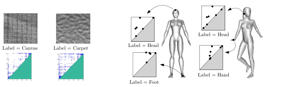
All kernels are handled with the LIBSVM [7] implementation of $C$ -SVM, and results are averaged over 10 runs on a 2.4GHz Intel Xeon E5530 Quad Core. The cost factor $C$ is cross-validated in the following grid: $\{0.001,0.01,0.1,1,10,100,1000\}$ . Table 1 summarizes the properties of the datasets we consider, namely number of labels, as well as training and test instances for each task. Figure 3 and 4 illustrate how we use persistence diagrams to represent complex data. We first describe the two baselines we considered, along with their parameterization, followed by our proposal.

Task	Training	Test	Labels
Orbit	175	75	5
Texture	240	240	24
Human	415	1618	8
Airplane	300	980	4
Ant	364	1141	5
Bird	257	832	4
FourLeg	438	1097	6
Octopus	334	1447	2
Fish	304	905	3

Table 1: Number of instances in the training set, the test set and number of labels.

Task	$k_{\rm PSS}$ ( $10^{-3}$ )	$k_{\rm PWG}$ (1000)	$k_{\rm SW}$ (6)
Orbit	$63.6\pm 1.2$	$77.7\pm 1.2$	${\bf 83.7}\pm 0.5$
Texture	${\bf 98.8}\pm 0.0$	$95.8\pm 0.0$	$96.1\pm 0.4$
Task	$k_{\rm PSS}$	$k_{\rm PWG}$	$k_{\rm SW}$
Human	$68.5\pm 2.0$	$64.2\pm 1.2$	${\bf 74.0}\pm 0.2$
Airplane	$65.4\pm 2.4$	$61.3\pm 2.9$	${\bf 72.6}\pm 0.2$
Ant	$86.3\pm 1.0$	$87.4\pm 0.5$	${\bf 92.3}\pm 0.2$
Bird	$67.7\pm 1.8$	${\bf 72.0}\pm 1.2$	$67.0\pm 0.5$
FourLeg	$67.0\pm 2.5$	$64.0\pm 0.6$	${\bf 73.0}\pm 0.4$
Octopus	$77.6\pm 1.0$	$78.6\pm 1.3$	${\bf 85.2}\pm 0.5$
Fish	$76.1\pm 1.6$	${\bf 79.8}\pm 0.5$	$75.0\pm 0.4$

Table 2: Classification accuracies (%) for the benchmark applications.

Task	$k_{\rm PSS}$ ( $10^{-3}$ )	$k_{\rm PWG}$ (1000)	$k_{\rm SW}$ (6)
Orbit	$N(124\pm 8.4)$	$N(144\pm 14)$	$415\pm 7.9+NC$
Texture	$N(165\pm 27)$	$N(101\pm 9.6)$	$482\pm 68+NC$
Task	$k_{\rm PSS}$	$k_{\rm PWG}$	$k_{\rm SW}$	$k_{\rm SW}$ (10)
Human	$N(29\pm 0.3)$	$N(318\pm 22)$	$2270\pm 336+NC$	$107\pm 14+NC$
Airplane	$N(0.8\pm 0.03)$	$N(5.6\pm 0.02)$	$44\pm 5.4+NC$	$10\pm 1.6+NC$
Ant	$N(1.7\pm 0.01)$	$N(12\pm 0.5)$	$92\pm 2.8+NC$	$16\pm 0.4+NC$
Bird	$N(0.5\pm 0.01)$	$N(3.6\pm 0.02)$	$27\pm 1.6+NC$	$6.6\pm 0.8+NC$
FourLeg	$N(10\pm 0.07)$	$N(113\pm 13)$	$604\pm 25+NC$	$52\pm 3.2+NC$
Octopus	$N(1.4\pm 0.01)$	$N(11\pm 0.8)$	$75\pm 1.4+NC$	$14\pm 2.1+NC$
Fish	$N(1.2\pm 0.004)$	$N(9.6\pm 0.03)$	$72\pm 4.8+NC$	$12\pm 1.1+NC$

Table 3: Gram matrices computation time (s) for the benchmark applications. As explained in the text,

N

represents the size of the set of possible parameters, and we have

N=13

for

k_{\rm PSS}

N=5\times 5\times 5=125

for

k_{\rm PWG}

and

N=3\times 5=15

for

k_{\rm SW}

C

is a constant that depends only on the training size. In all our applications, it is less than

0.1

PSS.

The Persistence Scale Space kernel $k_{\rm PSS}$ [34] is defined as the scalar product of the two solutions of the heat diffusion equation with initial Dirac sources located at the points of the persistence diagram. It has the following closed form expression:

k_{\rm PSS}(\mathrm{Dg}_{1},\mathrm{Dg}_{2})=\frac{1}{8\pi t}\sum_{p\in\mathrm{Dg}_{1}}\sum_{q\in\mathrm{Dg}_{2}}{\rm exp}\left(-\frac{\|p-q\|^{2}}{8t}\right)-{\rm exp}\left(-\frac{\|p-\bar{q}\|^{2}}{8t}\right),

where $\bar{q}=(y,x)$ is the symmetric of $q=(x,y)$ along the diagonal. Since there is no clear heuristic on how to tune $t$ , this parameter is chosen in the applications by ten-fold cross-validation with random 50%-50% training-test splits and with the following set of $N_{\rm PSS}=13$ values: $0.001$ , $0.005$ , $0.01$ , $0.05$ , $0.1$ , $0.5$ , $1$ , $5$ , $10$ , $50$ , $100$ , $500$ and $1000$ .

PWG.

Let $K,p>0$ and $\mathrm{Dg}_{1}$ and $\mathrm{Dg}_{2}$ be two persistence diagrams. Let $k_{\rho}$ be the Gaussian kernel with parameter $\rho>0$ . Let $\mathcal{H}_{\rho}$ be the RKHS associated to $k_{\rho}$ .

Let $\mu_{1}=\sum_{x\in\mathrm{Dg}_{1}}{\rm arctan}(K{\rm pers}(x)^{p})k_{\rho}(\cdot,x)\in\mathcal{H}_{\rho}$ be the kernel mean embedding of $\mathrm{Dg}_{1}$ weigthed by the diagonal distances. Let $\mu_{2}$ be defined similarly. Let $\tau>0$ . The Persistence Weighted Gaussian kernel $k_{\rm PWG}$ [23, 24] is defined as the Gaussian kernel with parameter $\tau$ on $\mathcal{H}_{\rho}$ :

k_{\rm PWG}(\mathrm{Dg}_{1},\mathrm{Dg}_{2})={\rm exp}\left(-\frac{\|\mu_{1}-\mu_{2}\|_{\mathcal{H}_{\rho}}}{2\tau^{2}}\right).

The authors in [23] provide heuristics to compute $K$ , $\rho$ and $\tau$ and give a rule of thumb to tune $p$ . Hence, in the applications we select $p$ according to the rule of thumb, and we use ten-fold cross-validation with random 50%-50% training-test splits to chose $K$ , $\rho$ and $\tau$ . The ranges of possible values is obtained by multiplying the values computed with the heuristics with the following range of $5$ factors: $0.01$ , $0.1$ , $1$ , $10$ and $100$ , leading to $N_{\rm PWG}=5\times 5\times 5=125$ different sets of parameters.

Parameters for $k_{\rm SW}$ .

The kernel we propose has only one parameter, the bandwidth $\sigma$ in Eq. 5, which we choose using ten-fold cross-validation with random 50%-50% training-test splits. The range of possible values is obtained by computing the squareroot of the median, the first and the last deciles of all ${\rm SW}(\mathrm{Dg}_{i},\mathrm{Dg}_{j})$ in the training set, then by multiplying these values by the following range of $5$ factors: $0.01$ , $0.1$ , $1$ , $10$ and $100$ , leading to $N_{\rm SW}=5\times 3=15$ possible values.

Parameter Tuning.

The bandwidth of $k_{\rm SW}$ is, in practice, easier to tune than the parameters of its two competitors when using grid search. Indeed, as is the case for all infinitely divisible kernels, the Gram matrix does not need to be recomputed for each choice of $\sigma$ , since it only suffices to compute all the Sliced Wasserstein distances between persistence diagrams in the training set once. On the contrary, neither $k_{\rm PSS}$ nor $k_{\rm PWG}$ share this property, and require recomputations for each hyperparameter choice. Note however that this improvement may no longer hold if one uses other methods to tune parameters. For instance, using $k_{\rm PWG}$ without cross-validation is possible with the heuristics given by the authors in [23], and leads to smaller training times, but also to worse accuracies.

4.1 3D shape segmentation

Our first task, whose goal is to produce point classifiers for 3D shapes, follows that presented in [6].

Data.

We use some categories of the mesh segmentation benchmark of Chen et al. [12], which contains 3D shapes classified in several categories (“airplane”, “human”, “ant”…). For each category, our goal is to design a classifier that can assign, to each point in the shape, a label that describes the relative location of that point in the shape. For instance, possible labels are, for the human category, “head”, “torso”, “arm”… To train classifiers, we compute a persistence diagram per point using the geodesic distance function to this point—see [6] for details. We use 1-dimensional persistent homology (0-dimensional would not be informative since the shapes are connected, leading to solely one point with coordinates $(0,+\infty)$ per persistence diagram). For each category, the training set contains one hundredth of the points of the first five 3D shapes, and the test set contains one hundredth of the points of the remaining shapes in that category. Points in training and test sets are evenly sampled. See Figure 4. Here, we focus on comparison between persistence diagrams, and not on achieving state-of-the-art results. It has been proven that persistence diagrams bring complementary information to classical descriptors in this task—see [6], hence reinforcing their discriminative power with appropriate kernels is of great interest. Finally, since data points are in $\mathbb{R}^{3}$ , we set the $p$ parameter of $k_{\rm PWG}$ to $5$ .

Results.

Classification accuracies are given in Table 2. For most categories, $k_{\rm SW}$ outperforms competing kernels by a significant margin. The variance of the results over the run is also less than that of its competitors. However, training times are not better in general. Hence, we also provide the results for an approximation of $k_{\rm SW}$ with $10$ directions. As one can see from Table 2 and from Figure 5, this approximation leaves the accuracies almost unchanged, while the training times become comparable with the ones of the other competitors. Moreover, according to Figure 5, using even less directions would slightly decrease the accuracies, but still outperform the competitors performances, while decreasing even more the training times.

4.2 Orbit recognition

In our second experiment, we use synthetized data. The goal is to retrieve parameters of dynamical system orbits, following an experiment proposed in [1].

Data.

We study the linked twist map, a discrete dynamical system modeling fluid flow. It was used in [19] to model flows in DNA microarrays. Its orbits can be computed given a parameter $r>0$ and initial positions $(x_{0},y_{0})\in[0,1]\times[0,1]$ as follows:

\left\{\begin{array}[]{l}x_{n+1}=x_{n}+ry_{n}(1-y_{n})\ \ \ \ \ \ \ \ \ \ \ {\rm mod}\ 1\\ y_{n+1}=y_{n}+rx_{n+1}(1-x_{n+1})\ \ \ {\rm mod}\ 1\end{array}\right.

Depending on the values of $r$ , the orbits may exhibit very different behaviors. For instance, as one can see in Figure 3, when $r$ is 3.5, there seems to be no interesting topological features in the orbit, while voids form for $r$ parameters around 4.3. Following [1], we use 5 different parameters $r=2.5,3.5,4,4.1,4.3$ , that act as labels. For each parameter, we generate 100 orbits with 1000 points and random initial positions. We then compute the persistence diagrams of the distance functions to the point clouds with the GUDHI library [39] and we use them (in all homological dimensions) to produce an orbit classifier that predicts the parameter values, by training over a 70%-30% training-test split of the data. Since data points are in $\mathbb{R}^{2}$ , we set the $p$ parameter of $k_{\rm PWG}$ to $4$ .

Results.

Since the persistence diagrams contain thousands of points, we use kernel approximations to speed up the computation of the Gram matrices. In order for the approximation error to be bounded by $10^{-3}$ , we use an approximation of $k_{\rm SW}$ with $6$ directions (as one can see from Figure 5, this has a small impact on the accuracy), we approximate $k_{\rm PWG}$ with $1000$ random Fourier features [32], and we approximate $k_{\rm PSS}$ using Fast Gauss Transform [27] with a normalized error of $10^{-10}$ . One can see from Table 2 that the accuracy is increased a lot with $k_{\rm SW}$ . Concerning training times, there is also a large improvement since we tune the parameters with grid search. Indeed, each Gram matrix needs not be recomputed for each parameter when using $k_{\rm SW}$ .

4.3 Texture classification

Our last experiment is inspired from [34] and [26]. We use the OUTEX00000 data base [28] for texture classification.

Data.

persistence diagrams are obtained for each texture image by computing first the sign component of CLBP descriptors [17] with radius $R=1$ and $P=8$ neighbors for each image, and then compute the persistent homology of this descriptor using the GUDHI library [39]. See Figure 4. Note that, contrary to the experiment of [34], we do not downsample the images to $32\times 32$ images, but keep the original $128\times 128$ images. Following [34], we restrict the focus to 0-dimensional persistent homology. We also use the first 50%-50% training-test split given in the database to produce classifiers. Since data points are in $\mathbb{R}^{2}$ , we set the $p$ parameter of $k_{\rm PWG}$ to $4$ .

Results

We use the same approximation procedure as in Section 4.2. According to Figure 5, even though the approximation of ${\rm SW}$ is rough, this has again a small impact on the accuracy, while reducing the training time by a significant margin. As one can see from Table 2, using $k_{\rm PSS}$ leads to almost state-of-the-art results [28, 17], closely followed by the accuracies of $k_{\rm SW}$ and $k_{\rm PWG}$ . The best timing is given by $k_{\rm SW}$ , again because we use grid search. Hence, $k_{\rm SW}$ almost achieves the best result, and its training time is better than the ones of its competitors, due to the grid search parameter tuning.

Figure 6: We show how the metric

d_{1}

is distorted. Each point represents a pair of persistence diagrams and its abscissae is the first diagram distance between them. Depending on the point color, its ordinate is the logarithm of the distance between persistence diagrams in the RKHS induced by either

k_{\rm PSS}

(blue points),

k_{\rm PWG}

(green points),

k_{\rm SW}

(red points) and a Gaussian kernel on

d_{1}

(black points).

4.4 Metric Distortion.

To illustrate the equivalence theorem, we also show in Figure 6 a scatter plot where each point represents the comparison of two persistence diagrams taken from the Airplane segmentation data set. Similar plots can be obtained with the other datasets considered here. For all points, the x-axis quantifies the first diagram distance $d_{1}$ for that pair, while the y-axis is the logarithm of the RKHS distance induced by either $k_{\rm SW}$ , $k_{\rm PSS}$ , $k_{\rm PWG}$ or a Gaussian kernel directly applied to $d_{1}$ , to obtain comparable quantities. We use the parameters given by the cross-validation procedure described above. One can see that the distances induced by $k_{\rm SW}$ are less spread than the others, suggesting that the metric induced by $k_{\rm SW}$ is more discriminative. Moreover the distances given by $k_{\rm SW}$ and the Gaussian kernel on $d_{1}$ exhibit the same behavior, suggesting that $k_{\rm SW}$ is the best natural equivalent of a Gaussian kernel for persistence diagrams.

5 Conclusion

In this article, we introduce the Sliced Wasserstein kernel, a new kernel for persistence diagrams that is provably equivalent to the first diagram distance between persistence diagrams. We provide fast algorithms to approximate it, and show on several datasets substantial improvements in accuracy and training times (when tuning parameters is done with grid search) over competing kernels. A particularly appealing property of that kernel is that it is infinitely divisible, substantially facilitating the tuning of parameters through cross validation.

Acknowledgements.

SO was supported by ERC grant Gudhi and by ANR project TopData. MC was supported by a chaire de l’IDEX Paris Saclay.

References

[1] Henry Adams, Tegan Emerson, Michael Kirby, Rachel Neville, Chris Peterson, Patrick Shipman, Sofya Chepushtanova, Eric Hanson, Francis Motta, and Lori Ziegelmeier. Persistence Images: A Stable Vector Representation of Persistent Homology. Journal of Machine Learning Research, 18(8):1–35, 2017.
[2] Ulrich Bauer and Michael Lesnick. Induced matchings and the algebraic stability of persistence barcodes. Journal of Computational Geometry, 6(2):162–191, 2015.
[3] Christian Berg, Jens Christensen, and Paul Ressel. Harmonic Analysis on Semigroups: Theory of Positive Definite and Related Functions. Springer, 1984.
[4] Peter Bubenik. Statistical Topological Data Analysis using Persistence Landscapes. Journal of Machine Learning Research, 16:77–102, 2015.
[5] Gunnar Carlsson, Vin de Silva, and Dmitriy Morozov. Zigzag Persistent Homology and Real-valued Functions. In Proceedings of the 25th Symposium on Computational Geometry, pages 247–256, 2009.
[6] Mathieu Carrière, Steve Oudot, and Maks Ovsjanikov. Stable Topological Signatures for Points on 3D Shapes. Computer Graphics Forum, 34, 2015.
[7] C. Chang and C. Lin. LIBSVM: A library for support vector machines. ACM Transactions on Intelligent Systems and Technology, 2:1–27, 2011. Software available at http://www.csie.ntu.edu.tw/~cjlin/libsvm.
[8] Frédéric Chazal, David Cohen-Steiner, Marc Glisse, Leonidas Guibas, and Steve Oudot. Proximity of Persistence Modules and their Diagrams. In Proceedings of the 25th Symposium on Computational Geometry, pages 237–246, 2009.
[9] Frédéric Chazal, David Cohen-Steiner, Leonidas Guibas, Facundo Mémoli, and Steve Oudot. Gromov-Hausdorff Stable Signatures for Shapes using Persistence. Computer Graphics Forum, pages 1393–1403, 2009.
[10] Frédéric Chazal, Vin de Silva, Marc Glisse, and Steve Oudot. The Structure and Stability of Persistence Modules. Springer, 2016.
[11] Frédéric Chazal, Vin de Silva, and Steve Oudot. Persistence stability for geometric complexes. Geometriae Dedicata, pages 1–22, 2013.
[12] X. Chen, A. Golovinskiy, and T. Funkhouser. A Benchmark for 3D Mesh Segmentation. ACM Transactions on Graphics, 28(3):1–12, 2009.
[13] David Cohen-Steiner, Herbert Edelsbrunner, and John Harer. Stability of Persistence Diagrams. Discrete and Computational Geometry, 37(1):103–120, 2007.
[14] Barbara di Fabio and Massimo Ferri. Comparing persistence diagrams through complex vectors. CoRR, abs/1505.01335, 2015.
[15] Herbert Edelsbrunner and John Harer. Computational Topology: an introduction. AMS Bookstore, 2010.
[16] Aasa Feragen, François Lauze, and Søren Hauberg. Geodesic exponential kernels: When curvature and linearity conflict. In IEEE Conference on Computer Vision and Pattern Recognition, pages 3032–3042, 2015.
[17] Zhenhua Guo, Lei Zhang, and David Zhang. A completed modeling of local binary pattern operator for texture classification. IEEE Transaction on Image Processing, pages 1657–1663, 2010.
[18] Juha Heinonen. Lectures on Analysis on Metric Spaces. Springer, 2001.
[19] Jan-Martin Hertzsch, Rob Sturman, and Stephen Wiggins. DNA microarrays: design principles for maximizing ergodic, chaotic mixing. In Small, volume 3, pages 202–218, 2007.
[20] Yasuaki Hiraoka, Takenobu Nakamura, Akihiko Hirata, Emerson Escolar, Kaname Matsue, and Yasumasa Nishiura. Hierarchical structures of amorphous solids characterized by persistent homology. In Proceedings of the National Academy of Science, volume 26, 2016.
[21] Soheil Kolouri, Yang Zou, and Gustavo Rohde. Sliced Wasserstein Kernels for Probability Distributions. In IEEE Conference on Computer Vision and Pattern Recognition, pages 5258–5267, 2016.
[22] Hermann König. Eigenvalue Distribution of Compact Operators. Operator Theory: Advances and Applications. Birkhäuser, 1986.
[23] Genki Kusano, Kenji Fukumizu, and Yasuaki Hiraoka. Persistence Weighted Gaussian Kernel for Topological Data Analysis. In Proceedings of the 33rd International Conference on Machine Learning, pages 2004–2013, 2016.
[24] Genki Kusano, Kenji Fukumizu, and Yasuaki Hiraoka. Kernel method for persistence diagrams via kernel embedding and weight factor. CoRR, abs/1706.03472, 2017.
[25] Roland Kwitt, Stefan Huber, Marc Niethammer, Weili Lin, and Ulrich Bauer. Statistical Topological Data Analysis - A Kernel Perspective. In Advances in Neural Information Processing Systems 28, pages 3070–3078, 2015.
[26] Chunyuan Li, Maks Ovsjanikov, and Frédéric Chazal. Persistence-Based Structural Recognition. In IEEE Conference on Computer Vision and Pattern Recognition, pages 2003–2010, 2014.
[27] Vlad Morariu, Balaji Srinivasan, Vikas Raykar, Ramani Duraiswami, and Larry Davis. Automatic online tuning for fast Gaussian summation. In Advances in Neural Information Processing Systems 21, pages 1113–1120, 2009.
[28] Timo Ojala, Topi Mäenpää, Matti Pietikäinen, Jaakko Viertola, Juha Kyllönen, and Sami Huovinen. Outex - new framework for empirical evaluation of texture analysis algorithms. In Proceedings of the 16th International Conference on Pattern Recognition, pages 701–706, 2002.
[29] Steve Oudot. Persistence Theory: From Quiver Representations to Data Analysis. Number 209 in Mathematical Surveys and Monographs. American Mathematical Society, 2015.
[30] Tullia Padellini and Pierpaolo Brutti. Supervised Learning with Indefinite Topological Kernels. CoRR, abs/1709.07100, 2017.
[31] Julien Rabin, Gabriel Peyré, Julie Delon, and Marc Bernot. Wasserstein barycenter and its application to texture mixing. In International Conference on Scale Space and Variational Methods in Computer Vision, pages 435–446, 2011.
[32] Ali Rahimi and Benjamin Recht. Random Features for Large-Scale Kernel Machines. In Advances in Neural Information Processing Systems 20, pages 1177–1184, 2008.
[33] Jan Reininghaus, Stefan Huber, Ulrich Bauer, and Roland Kwitt. A Stable Multi-Scale Kernel for Topological Machine Learning. CoRR, abs/1412.6821, 2014.
[34] Jan Reininghaus, Stefan Huber, Ulrich Bauer, and Roland Kwitt. A Stable Multi-Scale Kernel for Topological Machine Learning. In IEEE Conference on Computer Vision and Pattern Recognition, 2015.
[35] Vanessa Robins and Katharine Turner. Principal Component Analysis of Persistent Homology Rank Functions with case studies of Spatial Point Patterns, Sphere Packing and Colloids. Physica D: Nonlinear Phenomena, 334:1–186, 2016.
[36] Filippo Santambrogio. Optimal transport for applied mathematicians. Springer, 2015.
[37] Gurjeet Singh, Facundo Mémoli, Tigran Ishkhanov, Guillermo Sapiro, Gunnar Carlsson, and Dario Ringach. Topological analysis of population activity in visual cortex. Journal of Vision, 8, 2008.
[38] Ingo Steinwart and Clint Scovel. Mercer’s theorem on general domains: on the interaction between measures, kernels, and RKHSs. Constructive Approximation, 35:363–417, 2012.
[39] The GUDHI Project. GUDHI User and Reference Manual. GUDHI Editorial Board, 2015.
[40] Katharine Turner, Yuriy Mileyko, Sayan Mukherjee, and John Harer. Fréchet Means for Distributions of Persistence Diagrams. Discrete and Computational Geometry, 52(1):44–70, 2014.
[41] Cédric Villani. Optimal transport : old and new. Springer, 2009.

		$\displaystyle\mathcal{W}(\mu_{1}^{\theta}+\mu_{2\Delta}^{\theta},\mu_{2}^{\theta}+\mu_{1\Delta}^{\theta})=\sum_{(x,y)\in\gamma^{*}}\|x-y\|$
		$\displaystyle\leq\sum_{(\pi_{\theta}(p),\pi_{\theta}(q))\in\gamma_{\theta}}\|\langle p,\theta\rangle-\langle q,\theta\rangle\|{\rm\ since\ }\gamma_{\theta}{\rm\ is\ not\ the\ optimal\ matching\ between\ }\mathrm{Dg}_{1}^{\theta}{\rm\ and\ }\mathrm{Dg}_{2}^{\theta}$
		$\displaystyle\leq\sum_{(\pi_{\theta}(p),\pi_{\theta}(q))\in\gamma_{\theta}}\\|p-q\\|_{2}\text{ by the Cauchy-Schwarz inequality since }\\|\theta\\|_{2}=1$
		$\displaystyle\leq\sqrt{2}\sum_{(\pi_{\theta}(p),\pi_{\theta}(q))\in\gamma_{\theta}}\\|p-q\\|_{\infty}{\rm\ since\ }\\|\cdot\\|_{2}\leq\sqrt{2}\\|\cdot\\|_{\infty}$
		$\displaystyle\leq 2\sqrt{2}\sum_{(p,q)\in\gamma}\\|p-q\\|_{\infty}{\rm\ since\ }\\|\pi_{\Delta}(p)-\pi_{\Delta}(q)\\|_{\infty}\leq\\|p-q\\|_{\infty}$
		$\displaystyle=2\sqrt{2}d_{1}(\mathrm{Dg}_{1},\mathrm{Dg}_{2})$

	$\displaystyle{\rm SW}(\mathrm{Dg}_{1},\mathrm{Dg}_{2})$	$\displaystyle=\frac{1}{\pi}\int_{-\frac{\pi}{2}}^{\frac{\pi}{2}}\mathcal{W}(\mu_{1}^{\theta}+\mu_{2\Delta}^{\theta},\mu_{2}^{\theta}+\mu_{1\Delta}^{\theta})\ {\rm d}\theta=\frac{1}{\pi}\sum_{k=1}^{\|\Theta\|-1}\int_{\theta_{k}}^{\theta_{k+1}}\mathcal{W}(\mu_{1}^{\theta}+\mu_{2\Delta}^{\theta},\mu_{2}^{\theta}+\mu_{1\Delta}^{\theta})\ {\rm d}\theta$
		$\displaystyle\geq\left(\sum_{k=1}^{\|\Theta\|-1}\left(\theta_{k+1}-\theta_{k}\right)^{2}\right)\frac{d_{1}(\mathrm{Dg}_{1},\mathrm{Dg}_{2})}{2\pi^{2}}$
		$\displaystyle\geq\frac{\pi^{2}}{\|\Theta\|-1}\frac{d_{1}(\mathrm{Dg}_{1},\mathrm{Dg}_{2})}{2\pi^{2}}\text{ by the Cauchy-Schwarz inequality}$
		$\displaystyle\geq\frac{d_{1}(\mathrm{Dg}_{1},\mathrm{Dg}_{2})}{2M}$

Sliced Wasserstein Kernel for Persistence Diagrams

Abstract

1 Introduction

Persistence diagrams as features.

Related work.

Contributions.

2 Background

2.1 Persistent Homology

Distance between persistence diagrams.

Notation.

2.2 Kernel Methods

Negative Definite and RBF Kernels.

2.3 Wasserstein distance for unnormalized measures on ℝ\mathbb{R}

Proposition 2.1.

Proof.

Remark 2.2.

3 The Sliced Wasserstein Kernel

3.1 The Sliced Wasserstein Kernel

Definition 3.1.

Lemma 3.2.

Proof.

3.2 Metric Equivalence

3.2.1 Stability

Theorem 3.3.

Proof.

3.2.2 Discriminativity

Theorem 3.4.

Proof.

Proposition 3.5.

Proof.

3.3 Computation

Approximate computation.

Exact computation.

4 Experiments

Experimental setting

PSS.

PWG.

Parameters for kSWk_{\rm SW}.

Parameter Tuning.

4.1 3D shape segmentation

Data.

Results.

4.2 Orbit recognition

Data.

Results.

4.3 Texture classification

Data.

Results

4.4 Metric Distortion.

5 Conclusion

Acknowledgements.

References

2.3 Wasserstein distance for unnormalized measures on $\mathbb{R}$

Parameters for $k_{\rm SW}$ .