Chebyshev-Taylor parameterization of stable/unstable manifolds for periodic orbits: implementation and applications

J.D. Mireles James Maxime Murray Address: Department of mathematical sciences, Florida Atlantic University, 777 glades road
Boca Raton, Florida, 33431, United States of America
jmirelesjames@fau.edu
mmurray2016@fau.edu

Abstract

This paper develops Chebyshev-Taylor spectral methods for studying stable/unstable manifolds attached to periodic solutions of differential equations. The work exploits the parameterization method – a general functional analytic framework for studying invariant manifolds. Useful features of the parameterization method include the fact that it can follow folds in the embedding, recovers the dynamics on the manifold through a simple conjugacy, and admits a natural notion of a-posteriori error analysis. Our approach begins by deriving a recursive system of linear differential equations describing the Taylor coefficients of the invariant manifold. We represent periodic solutions of these equations as solutions of coupled systems of boundary value problems. We discuss the implementation and performance of the method for the Lorenz system, and for the planar circular restricted three and four body problems. We also illustrate the use of the method as a tool for computing cycle-to-cycle connecting orbits.

Key words. periodic orbit, (un)stable manifold, parameterization method, boundary value problems, automatic differentiation, Chebyshev polynomials

1 Introduction

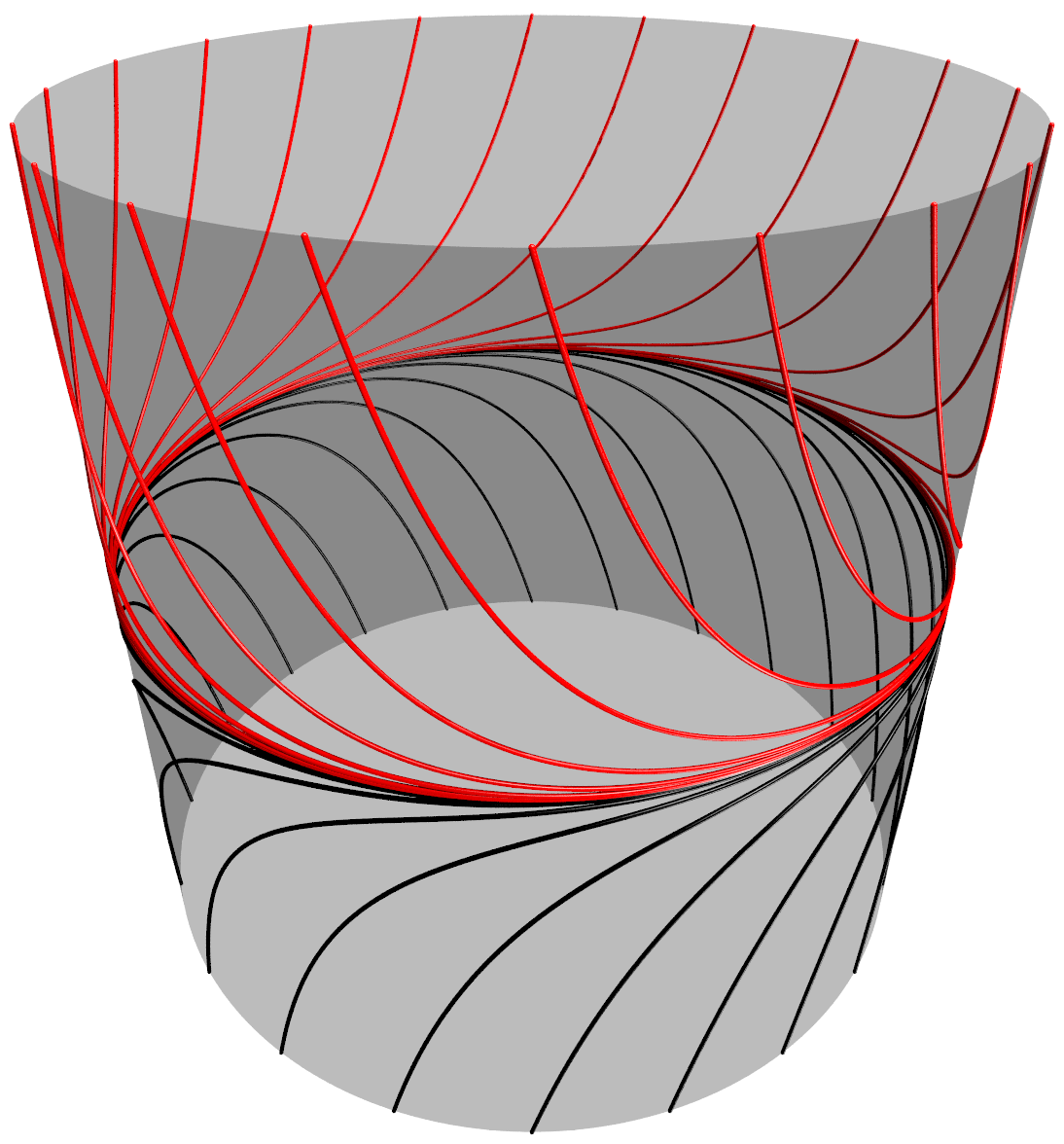
Periodic solutions of differential equations are the basic building blocks of recurrence in nonlinear dynamics. Moreover, hyperbolic periodic orbits and their heteroclinic/homoclinic connections are natural generators of chaotic motions. Since a heteroclinic/homoclinic orbit will approach a periodic solution along its local stable/unstable manifolds, computational methods for studying these manifolds are of great interest. A schematic description of the stable manifold of a periodic orbit, beside an actual stable manifold in the Lorenz system are illustrated in Figure 1. See any of the works Canalias and Masdemont, [2006]; Font et al., [2009]; Jorba, [1999]; Jorba and Masdemont, [1999]; Jorba and Villanueva, [1998]; Krauskopf et al., [2005]; Masdemont, [2011]; Osinga, [2003]; Simó, [1998]; Simó, [1988]; Simó, [1989] for more discussion, but we caution that any such list will hardly scratch the surface of the relevant literature.

The stable/unstable normal bundles of a periodic solution approximate the stable/unstable manifolds to first order, and these bundles are obtained by studying the equations of first variation – or equivalently – by solving certain periodic eigenvalue problems. Higher order jets of the invariant manifold could be studied via higher order equations of variation, however the complexity of these equations grows exponentially with the order of the jet. More efficient methods for studying the jets are obtained by reformulating the invariant manifold as the solution of an operator equation, and studying the operator equation via numerical methods.

The parameterization method is a general functional analytic framework for studying invariant manifolds Cabré et al., 2003a []; Cabré et al., 2003b []; Cabré et al., [2005]; Canadell and Haro, [2014]; Figueras and Haro, [2012]; Figueras and Haro, [2013]; Haro and de la Llave, 2006a []; Haro and de la Llave, 2006b []; Haro and de la Llave, [2007] whose goal is to find a chart/covering map conjugating the dynamics on the invariant manifold to a simple and well understood model (correctly choosing this model is part of the method). By viewing the conjugacy as an operator equation for the unknown chart, the problem is susceptible to numerical methods. We will see below that the operator equation of interest in the present work is actually a PDE with prescribed periodic data.

This operator equation is referred to as the invariance equation. The unknown parameterization is not required to be the graph of a function, and hence is able to follow folds in the embedding. See again Figure 1. Since the invariance equation is based on a dynamical conjugacy, the parameterization method recovers the dynamics on the manifold in addition to the embedding. By now there is a small industry devoted to the parameterization method, and a review of the literature would take us far afield. We refer the interested reader to the recent book on the subject Haro et al., [2016], where many examples and much more complete discussion of the literature is found.

Refer to caption — Figure 1: The local stable manifold attached to a periodic orbit $\gamma(t)$ : (LEFT) schematic representation of the stable manifold, i.e. it is the union of all solutions accumulating at $\gamma$ as $t\to\infty$ (periodic orbit shown here as the green loop). The unstable manifold is the same but with orbits approaching the periodic orbit asymptotically in backward time. (RIGHT) local stable manifold of an actual periodic orbit near the Lorenz attractor. This manifold is computed using the techniques of the present work. In particular, changes in color in the figure indicate the transitions from one Chebyshev domain to another.

The present work is not the first numerical treatment of parameterized stable/unstable manifolds attached to periodic orbits, and indeed we build on the earlier studies of Cabré et al., [2005]; Castelli et al., [2015]; Guillamon and Huguet, [2009]; Huguet and de la Llave, [2013]. As in these earlier studies, we make a formal Taylor series arguments which analytically reduces the invariance equation before making any numerical computations. Since the coefficients of the Taylor series are themselves periodic functions, the formal power matching scheme leads to so called homological equations describing the unknown coefficients. In the present case of a periodic orbit, the homological equations are linear ordinary differential equations with periodic coefficients and periodic forcing. We solve these linear homological equations recursively using numerical spectral methods. By computing the formal series solution to high order we obtain an approximate solution which describes the stable/unstable manifold far from the periodic orbit.

In the earlier works just cited the differential equations – describing the periodic orbit, describing the normal bundles, and the homological equations describing the higher order jets – are all solved using Fourier spectral methods. Fourier methods are both efficient and accurate when applied to periodic solutions of moderate length. This efficiency is due in part to the fact that differentiation is a diagonal operation in the transform domain, and in part to the fact that the FFT speeds up evaluation of nonlinearities. However, the decay rate of the Fourier coefficients gets increasingly slow as the period/harmonic complexity of the orbit grow. In practice this means that it is necessary to compute more and more Fourier coefficients, and for long enough orbits the Fourier approximation becomes impractical.

There is much recent interest in numerical methods based on Chebyshev spectral approximation of solutions to boundary value problems. We refer the interested reader to Driscoll et al., [2008]; Platte and Trefethen, [2010]; Trefethen, [2007]; Trefethen, [2013] and the references discussed there in. The present work builds on techniques developed by a number of authors which use Chebyshev spectral methods to compute long periodic solutions of differential equations Gameiro et al., [2016]; Lessard and Reinhardt, [2014]; van den Berg and Sheombarsing, [2016]. The merit of this approach is that the Chebyshev spectral methods posess many of the advantages of Fourier series – for example differentiation is a tri-diagonal operation in the transform domain and the fast cosine transform is available for evaluating nonlinearities – but Chebyshev series apply to non-periodic boundary value problems. Treating a periodic solution as a series of coupled boundary value problems – on smaller domains – facilitates control of the decay rates of the coefficients.

Motivated by these developments, the present work applies Chebyshev methods not only the periodic orbit – but also to the computation of the normal bundles and the homological equations for the higher order jets. The result is a computational method for finding Chebyshev-Taylor expansions of the local stable/unstable manifolds attached to periodic orbits. Our method applies to more complicated orbits and their attached invariant manifolds than could be studied using only the Fourier-Taylor approach.

Remark 1.1 (Connecting orbits and extensions of local stable/unstable manifolds).

Of course computing local stable/unstable manifolds attached to periodic orbits is only a means to an end. In applications we are often interested in either using the local manifolds to compute connecting orbits, or to grow larger portions of the invariant manifold in order to study the global dynamics. While in the present work we do consider a number of example computations for connecting orbits, we do not make any serious attempt to numerically grow larger local manifolds. This is because the literature on computational methods for growing invariant manifolds is extensive and well developed. The interested reader will want to consult the review paper Krauskopf et al., [2005] for a thorough overview of the literature, and will find other powerful methods and fuller discussion in England et al., [2005]; Osinga, [2000]; Osinga, [2003]. We only note that the methods developed in the present work could be combined with existing continuation methods for even better results. This is especially true for methods which exploit the curvature or other differential geometric properties of the manifold.

Remark 1.2 (Automatic differentiation and polynomial nonlinearities).

Multiplication of Taylor and Chebyshev series is straight forward thanks to the Cauchy product in the former case and the discrete cosine convolution operation in the later. Then formal series manipulations for polynomial nonlinearities are especially transparent in Chebyshev-Taylor bases. In the present work we are interested in applications coming from celestial mechanics which involve non-polynomial vector fields. In order to simplify matters we exploit methods of automatic differentiation and transform to the polynomial setting, albeit in a higher dimensional phase space. This is discussed in detail in Section 2.3.

The use of automatic differentiation is a convenience rather than a necessity, as the FFT could be used to evaluate general nonlinearities. In fact, even after automatic differentiation we use the fast cosine transform to evaluate higher order polynomial nonlinearities in the present work. Nevertheless, the use of automatic differentiation in the present work simplifies the implementation details of our algorithms – as all our computations are reduced to Newton’s method for large polynomial systems. Automatic differentiation also simplifies a-posteriori error analysis for the method, which when followed to its logical conclusion provides mathematically rigorous validated error bounds for the parameterizations.

2 Review of the parameterization method

As already mentioned in the introduction, the parameterization method is much more general than what we actually use in the present work. We refer the reader again to the book Haro et al., [2016]. In the following section we review some basic notions in the very simple setting of an orientable local manifold associated with one stable/unstable Floquet exponent. Generalities such as multiple stable/unstable exponents, complex conjugate exponents, and non-orientable bundles are discussed in detail in Castelli et al., [2015]. The methods of the present work apply in these more general setting with only obvious modifications. We focus on the one dimensional case to simplify the exposition.

2.1 Parameterization of stable/unstable manifolds attached to periodic orbits

Let $\Omega\subset\mathbb{R}^{M}$ be an open set and $g\colon\Omega\to\mathbb{R}^{M}$ be a real analytic vector field. Suppose that $\gamma\colon\mathbb{R}\to\mathbb{R}^{M}$ is a $T$ -periodic solution of the first order ordinary differential equation

\dot{x}=g(x),

that is we assume that $\gamma^{\prime}(t)=g(\gamma(t))$ with $\gamma(t+T)=\gamma(t)$ for all $t\in\mathbb{R}$ . Suppose also that $\gamma$ has one stable Floquet exponent

\lambda\in\mathbb{R},\quad\quad\quad\mbox{with }\quad\quad\quad\lambda<0,

so that (by the stable manifold theorem) there exists a two dimensional manifold of solutions which converge exponentially fast to the periodic orbit $\gamma$ . Let $v\colon\mathbb{R}\to\mathbb{R}^{M}$ denote the stable normal bundle of $\gamma(t)$ , associated with the exponent $\lambda$ . We assume that $v$ is an orientable bundle, so that $v(t)$ is $T$ periodic as well. We note that $(v,\lambda)$ solve the eigenvalue problem

\frac{d}{dt}v(t)=Dg(\gamma(t))v(t)-\lambda v(t),

subject to some normalization, perhaps $\|v(t)\|=1$ for all $t\in\mathbb{R}$ (though in numerical applications we will choose other normalizations).

The goal of the parameterization method is to find a smooth function $P\colon[0,T]\times[-1,1]\to\mathbb{R}^{M}$ solving the invariance equation

\frac{\partial}{\partial t}P(t,\sigma)+\lambda\sigma\frac{\partial}{\partial\sigma}P(t,\sigma)=g(P(t,\sigma)),

(1)

subject to the first order constraints

P(t,0)=\gamma(t),

(2)

and

\frac{\partial}{\partial\sigma}P(t,0)=v(t).

(3)

Then geometric content of Equation (1) is illustrated in Figure 2, but one easily checks that the image of $P$ is a stable manifold.

Indeed, let $P$ be a smooth solution of Equation (1) subject to the first order constraints. Choose any $\sigma_{0}\in(-1,1)$ and define the curve $x\colon[0,\infty)\to\mathbb{R}^{M}$ by

x(t)=P(t,e^{\lambda t}\sigma_{0}).

Then

	$\displaystyle\frac{d}{dt}x(t)$	$\displaystyle=DP(t,e^{\lambda t}\sigma_{0})\left(\begin{array}[]{c}1\\ e^{\lambda t}\lambda\sigma_{0}\end{array}\right)$
		$\displaystyle=\frac{\partial}{\partial t}P(t,e^{\lambda t}\sigma_{0})+\lambda\sigma_{0}e^{\lambda t}\frac{\partial}{\partial\sigma}P(t,e^{\lambda t}\sigma_{0})$
		$\displaystyle=g(P(t,e^{\lambda t}\sigma_{0}))$
		$\displaystyle=g(x(t)),$

as $e^{\lambda t}\sigma_{0}\in(-1,1)$ for all $t\geq 0$ . Then $x(t)$ is a solution curve for the differential equation having $x(0)=P(0,\sigma_{0})$ . Moreover for any $t_{0}\in[0,L]$ , since $P$ is continuous we have that

	$\displaystyle\lim_{t\to\infty}P(t_{0},e^{\lambda t}\sigma_{0})$	$\displaystyle=P\left(t_{0},\lim_{t\to\infty}e^{\lambda t}\sigma_{0}\right)$
		$\displaystyle=P(t_{0},0)$
		$\displaystyle=\gamma(t_{0}),$

that is, a point on the image of $P$ accumulates at the periodic orbit $\gamma$ with asymptotic phase $\gamma(t_{0})$ . In particular, the image of $P$ is a local stable manifold for $\gamma$ .

One can actually prove more. For example if $P$ solves Equation (1) subject to the first order constraints, then $P$ actually satisfies the flow conjugacy

\displaystyle P(s+t,e^{\lambda t}\sigma)=\Phi(P(s,\sigma),t)

(4)

for all $t\geq 0$ . Here $\Phi$ is the flow generated by the vector field $g$ . The meaning of this flow conjugacy is illustrated in Figure 3. The proof of the flow conjugacy is given for example in Castelli et al., [2015]. In the same reference it is shown that solutions of Equation (1) are unique up to the choice of the eigenfunction $v(t)$ . (Any constant multiple of $v$ is a parameterization of the stable normal bundle, but up to this choice of scaling the solution is unique). If the solution $P$ exists, it is as regular as $g$ . In this case $P$ is real analytic if $g$ is Cabré et al., 2003b []; Cabré et al., [2005]. Moreover, in the case of one stable exponent, there exists a choice of scaling small enough that the solution $P$ exists, and is analytic. See Cabré et al., 2003a []; Cabré et al., [2005]; Huguet and de la Llave, [2013].

2.2 Formal series and the reduction to homological equations

Since $P$ exists and is analytic it makes sense to seek a power series solution

P(t,\sigma)=\sum_{\alpha=0}^{\infty}A_{\alpha}(t)\sigma^{\alpha},

(5)

where $\sigma\in(-1,1)$ and the functions $A_{\alpha}\colon\mathbb{R}\to\mathbb{R}^{M}$ are analytic and $T$ -periodic. Plugging the power series into Equation (1), expanding the nonlinearities, and matching like powers leads to equations for the unknown Taylor coefficient functions.

Example: the Lorenz system in the specific case of the Lorenz field we have that $M=3$ , and that the vector field $g$ is given by

g(x,y,z)=\left(\begin{array}[]{c}\sigma(y-x)\\ x\rho-xz-y\\ xy-\beta z\end{array}\right),

where $\beta,\rho,\sigma$ are positive constants. Suppose that $\gamma(t)=(x(t),y(t),z(t))$ is an analytic period- $T$ orbit with stable (or unstable) exponent $\lambda$ and that $v(t)=(v_{1}(t),v_{2}(t),v_{3}(t))$ is an analytic $T$ -periodic parameterization of the stable normal bundle. We look for

P(t,s)=\sum_{\alpha=0}^{\infty}A_{\alpha}(t)s^{\alpha}=\sum_{\alpha=0}^{\infty}\left(\begin{array}[]{c}a^{(1,\alpha)}(t)\\ a^{(2,\alpha)}(t)\\ a^{(3,\alpha)}(t)\end{array}\right)s^{\alpha}

Then

A_{0}(t)=\gamma(t),\quad\quad\quad\mbox{and}\quad\quad\quad A_{1}(t)=v(t).

Since

\frac{\partial}{\partial t}P(t,s)+\lambda s\frac{\partial}{\partial s}P(t,s)=\sum_{\alpha=0}^{\infty}\left(\frac{d}{dt}A_{\alpha}(t)+\alpha\lambda A_{\alpha}(t)\right)s^{\alpha},

and

\displaystyle g(P(t,s))

\displaystyle=\sum_{\alpha=0}^{\infty}\left(\begin{array}[]{c}\sigma\left(a^{(2,\alpha)}-a^{(1,\alpha)}\right)\\ \rho a^{(1,\alpha)}-a^{(2,\alpha)}-\sum_{\beta=0}^{\alpha}a^{(1,\alpha-\beta)}a^{(3,\beta)}\\ -\beta a^{(3,\alpha)}+\sum_{\beta=0}^{\alpha}a^{(1,\alpha-\beta)}a^{(2,\beta)}\end{array}\right)s^{\alpha},

equating and matching like powers of $s$ leads to

	$\displaystyle\frac{d}{dt}A_{\alpha}(t)+\alpha\lambda A_{\alpha}(t)$	$\displaystyle=\left(\begin{array}[]{c}\sigma\left(a^{(2,\alpha)}-a^{(1,\alpha)}\right)\\ \rho a^{(1,\alpha)}-a^{(2,\alpha)}-\sum_{\beta=0}^{\alpha}a^{(1,\alpha-\beta)}a^{(3,\beta)}\\ -\beta a^{(3,\alpha)}+\sum_{\beta=0}^{\alpha}a^{(1,\alpha-\beta)}a^{(2,\beta)}\end{array}\right)$
		$\displaystyle=\left(\begin{array}[]{c}\sigma\left(a^{(2,\alpha)}-a^{(1,\alpha)}\right)\\ \rho a^{(1,\alpha)}-a^{(2,\alpha)}-a^{(1,\alpha)}a^{(3,0)}-a^{(3,\alpha)}a^{(1,0)}\\ -\beta a^{(3,\alpha)}+a^{(1,\alpha)}a^{(2,0)}+a^{(2,\alpha)}a^{(1,0)}\end{array}\right)+\left(\begin{array}[]{c}0\\ -\sum_{\beta=1}^{\alpha-1}a^{(1,\alpha-\beta)}a^{(3,\beta)}\\ \sum_{\beta=1}^{\alpha-1}a^{(1,\alpha-\beta)}a^{(2,\beta)}\end{array}\right).$

Noting that

	$\displaystyle\left(\begin{array}[]{c}\sigma\left(a^{(2,\alpha)}-a^{(1,\alpha)}\right)\\ \rho a^{(1,\alpha)}-a^{(2,\alpha)}-a^{(1,\alpha)}a^{(3,0)}-a^{(3,\alpha)}a^{(1,0)}\\ -\beta a^{(3,\alpha)}+a^{(1,\alpha)}a^{(2,0)}+a^{(2,\alpha)}a^{(1,0)}\end{array}\right)$	$\displaystyle=\left[\begin{array}[]{ccc}-\sigma&\sigma&0\\ \rho-z(t)&1&-x(t)\\ y(t)&x(t)&-\beta\end{array}\right]A_{\alpha}(t)$
		$\displaystyle=Dg(\gamma(t))A_{\alpha}(t),$

define the functions $g_{\alpha}$ by

g_{\alpha}(A_{1}(t),\ldots,A_{\alpha-1}(t)):=\left(\begin{array}[]{c}0\\ -\sum_{\beta=1}^{\alpha-1}a^{(1,\alpha-\beta)}(t)a^{(3,\beta)}(t)\\ \sum_{\beta=1}^{\alpha-1}a^{(1,\alpha-\beta)}(t)a^{(2,\beta)}(t)\end{array}\right).

We write $g_{\alpha}(P)$ for short. Now we seek $A_{\alpha}(t)$ the $T$ -periodic solution of the equation

\frac{d}{dt}A_{\alpha}(t)-\left(Dg(\gamma(t))-\lambda\alpha\mbox{Id}\right)A_{\alpha}(t)=g_{\alpha}(P),

(6)

which we refer to as the homological equation for $P$ . Note that this is a linear inhomogeneous first order ordinary differential equation with periodic coefficients, and that the right hand side is independent of $A_{\alpha}$ . Indeed, $g_{\alpha}$ depends recursively on lower order terms. The Floquet theory guarantees that our homological equation has a unique periodic solution for each $\alpha\geq 2$ . Then we recursively solve the equations to order $N$ and have the approximate solution

P^{N}(t,s)=\sum_{\alpha=0}^{N}A_{\alpha}(t)s^{\alpha}.

Remark 2.1 (A-posteriori error analysis).

Truncation error analysis is treated carefully in Castelli et al., [2017]. Note that the analysis in that reference is independent of the basis used to represent $A_{\alpha}(t)$ : only the implementation exploits that these functions are given as Fourier series. Then the methods of the work just cited apply directly to the expansions used in the present work. The key to the analysis in Castelli et al., [2017] is that the approximation $P^{N}$ have small defect. In the present work we only check the defect numerically, and postpone to an upcoming work more careful analysis of the errors for our Chebyshev-Taylor approximations.

The calculations above generalizes to any polynomial vector field in the obvious way, and we have that the $A_{\alpha}$ satisfy homological equations of exactly the form given in Equation (6). Only the term $Dg(\gamma(t))$ and the form of the recursive functions $g_{\alpha}(P)$ depend explicitly on the form of the vector field $g$ . In the other examples in the present work we simply write down the correct homological equations and leave the derivations as an exercise for the interested reader.

2.3 A dynamical perspective on automatic differentiation

The term automatic differentiation refers to a whole suite of methods for managing the complexity of problems involving high order derivatives. These methods exploit the fact that differentiation and multiplication are related through the chain rule. For a general introduction and an overview of the literature we refer to Rall and Corliss, [1996]; Bücker and Corliss, [2006], though in the present work our use of the term is much closer to that of Chapter $2$ of Haro et al., [2016] and also Jorba and Zou, [2005]. See also Chapter $4.7$ of Knuth, [1998]. The discussion of the literature in this last reference is especially illuminating, though the reference does not use the “automatic differentiation” terminology.

While automatic differentiation can be viewed as a technique for computing transcendental functions of polynomials (where the result should again be expressed as a polynomial), automatic differentiation can also bee seen as a technique transforming non-polynomial into polynomial problems by appending additional polynomial differential equations. The solutions of the appended differential equations are required to give the non-polynomial terms of the original problem. When viewed this way it is possible to use automatic differentiation to solve problems involving Fourier and Chebyshev rather than just Taylor bases. Such extensions are discussed for example in Lessard et al., [2016], where automatic differentiation is simply viewed as a change of variables which transforms the given problem to a polynomial problem.

In general a change of variables will disturb the orbit structure of a differential equation, unless the change of variables induces a dynamical (semi)-conjugacy. This issue is considered at length in Kepley and Mireles James, [2017], where a dynamical systems interpretation of automatic differentiation is introduced. We adopt this interpretation here as well. So, suppose that $U\subset\mathbb{R}^{d}$ is an open set and that $f\colon U\to\mathbb{R}^{d}$ is a real analytic vector field with non-polynomial nonlinearity. From the perspective of the present work, the goal of automatic differentiation is to find a mapping $R\colon U\to\mathbb{R}^{D}$ with $D>d$ and a polynomial vector field $F\colon\mathbb{R}^{D}\to\mathbb{R}^{D}$ having that

\pi_{d}(R(\mathbf{x}))=\mathbf{x},

where $\pi_{d}\colon\mathbb{R}^{D}\to\mathbb{R}^{d}$ is the projection into the lower dimensional space, and that

DR(\mathbf{x})f(\mathbf{x})=F(R(\mathbf{x})),\quad\quad\quad\quad\mbox{for all }\mathbf{x}\in U.

(7)

This leads to the following observations.

$\bullet$

Since $\pi_{d}R=\mbox{Id}_{d}$ , it follows that

$\pi_{d}F(R(\mathbf{x}))=f(\mathbf{x}),$

so that the original field is recovered by projection.
$\bullet$

Equation (7) is an infinitesimal conjugacy, and implies that $R$ maps orbits of $f$ to orbits of $F$ . Moreover it says that graph of $R$ is invariant under the flow generated by $F$ .
$\bullet$

Then when we solve the differential equations given by $F$ with initial conditions on the graph of $R$ , we can recover the orbits of $f$ simply by projecting.

The procedure for choosing $R$ and $F$ is best illustrated through examples, but it is worth noting that $R$ will have the same domain as $f$ . So even though $F$ is polynomial and hence entire, the composition of $F\circ R$ will have the same singularities as $f$ .

Example: Consider the Kepler problem

	$\displaystyle x^{\prime}$	$\displaystyle=y$
	$\displaystyle y^{\prime}$	$\displaystyle=-\frac{M}{\|x\|^{3}}x.$

We introduce the new variable

z=\frac{1}{|x|}=\frac{1}{\sqrt{x^{2}}},

and note that away from the origin one has

z^{\prime}=\frac{d}{dt}(x^{2})^{-1/2}=\frac{-1}{2}\left(x^{2}\right)^{-3/2}2x^{\prime}=-z^{3}y.

Then taking

R(x,y)=\left(\begin{array}[]{c}x\\ y\\ \frac{1}{|x|}\end{array}\right),\quad\quad\quad\mbox{and}\quad\quad\quad F(x,y,z)=\left(\begin{array}[]{c}y\\ -Mz^{3}x\\ -z^{3}y\end{array}\right),

one easily checks the conjugacy Equation (7), and also that the first two components of $F\circ R$ recover $f$ . Solution curves of the vector field $F$ with initial conditions on the graph of $R$ recover solutions of the Kepler problem as long as they remain on the graph of $R$ . That is, if

\left(\begin{array}[]{c}x^{\prime}\\ y^{\prime}\\ z^{\prime}\end{array}\right)=F(x,y,z),\quad\quad\quad\mbox{and }\left(\begin{array}[]{c}x(0)\\ y(0)\\ z(0)\end{array}\right)=R(x_{0},y_{0}),

then $x(t),y(t)$ is a solution of the Kepler problems as long as $x(t),y(t),z(t)$ is on the graph of $R$ . Moreover, the trajectory leaves the graph of $R$ if and only if there is a collision in the the Kepler problem. This example is typical of automatic differentiation for problems in celestial mechanics. A thorough discussion – from the dynamical systems point of view – of automatic differentiation for the circular restricted four body problem is found in Kepley and Mireles James, [2017].

3 Chebyshev Expansion for Periodic Solutions of $\dot{u}(t)=h(u(t),t)$

The periodic orbit $\gamma$ , its stable/unstable normal bundle $v(t)$ , and the higher order Taylor coefficients $A_{\alpha}(t)$ for $2\leq\alpha\leq N$ are all periodic solutions of non-autonomous differential equations of the form

\displaystyle\dot{u}(t)=h(u(t),t),

with period $\tau$ , and where $h:\mathbb{R}^{M}\times\mathbb{R}\to\mathbb{R}^{M}$ . In each case we look for a solutions $v:[0,\tau]\to\mathbb{R}^{M}$ satisfying the boundary value problem

\displaystyle\begin{cases}\dot{v}(t)=h(v(t),t),\\ v(0)=v(\tau).\end{cases}

(8)

We develop a Chebyshev scheme to solve this class of problems.

To begin, break the solution into sub-pieces using the following mesh. Let $0=t_{0}<t_{1}<t_{2}<\ldots<t_{D}=\tau$ , and for $i=1,\ldots,D$ define $v^{i}(t)$ on $[t_{i-1},t_{i}]$ such that

v^{i}(t)=v(t).

Thus, each $v^{i}(t)$ is a solution of $\dot{u}(t)=h(u(t),t)$ . Moreover, at each of the points $t_{i}$ , $1\leq i\leq D-1$ , two different pieces are defined and they must agree. Then we impose the boundary conditions

\displaystyle\begin{cases}\dot{v}^{i}(t)=h(v^{i}(t),t),&\\ v^{i}(t_{i-1})=v^{i-1}(t_{i-1}),\end{cases}

(9)

for $i\neq 1$ , and to impose periodicity

\displaystyle\begin{cases}\dot{v}^{1}(t)=h(v^{1}(t),t),&\\ v^{1}(t_{0})=v^{D}(t_{D}).\end{cases}

We want to expand each piece $v^{i}(t)$ using Chebyshev polynomials. To do so, we first rescale the problem to the interval $[-1,1]$ . First, note that since there are no time dependence in $g$ (the original system for which we compute the periodic orbit) we can translate the time domain to some interval $[-L_{i},L_{i}]$ and then rescale time $t\mapsto\frac{t}{L_{i}}$ , so that the solution satisfies

\displaystyle\dot{v}^{i}(t)=L_{i}h(v^{i}(t),t),

(10)

for all $i=1,\ldots,D$ .

For the time varying case, i.e. the case of the bundles and the homological equations, the solution will depend on the lower power $\alpha$ of the coefficient in question. Since the bundles and Taylor coefficients of the parameterization are all periodic with the same period, we choose a fixed mesh for all the problems. That is, the number of subdomains $D$ will be the same at every step. Moreover each $L_{i}$ is a fixed proportion of the global period. So $L_{i}=p_{i}L$ for $p_{i}\in(0,1]$ some given constant. In applications unless otherwise specified we use a uniform mesh, so that $p_{i}=\frac{1}{D}$ for all $i$ .

We introduce a Chebyshev expansion for each sub-piece $v^{i}$ that are now defined on $[-1,1]$ . Let $v^{(i,j)}:[-1,1]\to\mathbb{R}$ denote the $j-$ th component of $v^{i}$ for all $i=1,\ldots,M$ . For any $i=1,\ldots,D$ and $j=1,\ldots,M$ , we set

\displaystyle v^{(i,j)}(t)\,\stackrel{{\scriptstyle\mbox{\tiny{\raisebox{0.0pt}[0.0pt][0.0pt]{def}}}}}{{=}}\,a_{0}^{(i,j)}+2\sum_{k=1}^{\infty}a_{k}^{(i,j)}T_{k}(t),

(11)

where $T_{k}$ is the $k-$ th Chebyshev polynomial, which are defined as follows.

Definition 3.1.

The Chebyshev polynomials $T_{k}:[-1,1]\rightarrow\mathbb{R}$ , $k=0,1,2,\dots$ are defined by $T_{0}(t)=1$ and $T_{1}(t)=t$ and the recurrence relation

T_{k+1}(t)=2tT_{k}(t)-T_{k-1}(t),\quad k\geq 1.

It is well known that these polynomials satisfy $T_{k}(\cos\theta)=\cos(k\theta)$ , a fact which can be used to prove further results relating the Chebyshev series to results from Fourier analysis.

Definition 3.2.

We denote the set of unknown Chebyshev coefficients of the full periodic orbit $v$ by

A=\left(A^{(1)},A^{(2)},\ldots,A^{(D)}\right).

So that for every $i=1,2\ldots,M$ , $A^{(i)}$ represent the set of coefficients of the $i-$ th piece of $v$ defined on the interval $[t_{i-1},t_{i}]$ . Moreover, for a fixed $k$ , $A_{k}^{(i)}\in\mathbb{R}^{M}$ since each has an image included in $\mathbb{R}^{M}$ , which are all expanded using distinct Chebyshev expansions. Finally, $a_{k}^{(i,j)}$ denotes the $k-$ th coefficient of the $j-$ th dimension of $v^{i}$ .

To rewrite the system as an operator defined on the set $A$ we integrate (10) from $-1$ to $t$ and obtain

\displaystyle v^{i}(t)-v^{i}(-1)=L_{i}\int_{-1}^{t}h(v^{i}(s),s)ds.

(12)

Note that $h:[-1,1]\to\mathbb{R}^{M}$ , since it depends on the lower and current term of the expansion of the parameterization which all are defined on $[-1,1]$ after rescaling time. Thus it can also be expanded using Chebyshev polynomials. We set

h^{j}(v^{i}(t),t)=c_{0}^{(i,j)}+2\sum_{k=1}^{\infty}c_{k}^{(i,j)}T_{k}(t),

and substitute both Chebyshev expansions in (12) to get an equation whose only time dependence is in the Chebyshev polynomials themselves/the integral. We use the recurrence formulas for the integral of the Chebyshev polynomials and rewrite the initial condition so that after simplification the Chebyshev coefficients need to satisfy a set of conditions defined in the space of Chebyshev coefficients. That is, for all $i=1,\ldots,D$ , $j=1,\ldots,M$ and $k\geq 0$ , we define

f_{k}^{(i,j)}(L,A)=0.

Each $f_{k}^{(i,j)}(L,A)$ is given by

\displaystyle f_{k}^{(i,j)}(L,A)\,\stackrel{{\scriptstyle\mbox{\tiny{\raisebox{0.0pt}[0.0pt][0.0pt]{def}}}}}{{=}}\,\begin{cases}\displaystyle\left(a_{0}^{(i-1,j)}+2\sum_{l=1}^{\infty}a_{l}^{(i-1,j)}\right)-\left(a_{0}^{(i,j)}+2\sum_{l=1}^{\infty}a_{l}^{(i,j)}(-1)^{l}\right),&\mbox{if}\;k=0\\ 2ka_{k}^{(i,j)}+L_{i}c_{k\pm 1}^{(i,j)},&\mbox{if}\;k>0.\end{cases}

(13)

Definition 3.3.

We write $c_{k\pm 1}$ to denote $c_{k\pm 1}:=c_{k+1}-c_{k-1}$ .

We omit the derivation of the operators $f_{k}^{(i,j)}$ . For further details, and to see why the term $k=0$ does not depend on the vector field but only on the boundary condition, we refer to Lessard and Reinhardt, [2014].

The boundary condition provides the initial component for the new problem, that is for the case $f_{0}^{(i,j)}$ . So we use the form given in Equation (13) for every subintervals except for the case $i=1$ , for which we use

\displaystyle f_{0}^{(1,j)}(L,A)=\left(a_{0}^{(D,j)}+2\sum_{l=1}^{\infty}a_{l}^{(D,j)}\right)-\left(a_{0}^{(1,j)}+2\sum_{l=1}^{\infty}a_{l}^{(1,j)}(-1)^{l}\right).

(14)

The operator involves coefficients of the Chebyshev expansion of $h$ , which we need to write in terms of the unknowns $A$ . Since the Chebyshev expansion of a sum (or difference) of two functions $f$ and $g$ will be given by the sum (or difference) of the Chebyshev coefficients of $f$ and $g$ , and since we assume $h$ to be polynomial, the only other case to handle is a product. We use the following Lemma.

Lemma 3.4.

If $f(t)$ and $g(t)$ are expanded with Chebyshev series so that

f(t)=a_{0}+2\sum_{k=1}^{\infty}a_{k}T_{k}(t)\quad\mbox{and}\quad g(t)=b_{0}+2\sum_{k=1}^{\infty}b_{k}T_{k}(t),

then $f(t)g(t)=(a\ast b)_{0}+2\displaystyle\sum_{k=1}^{\infty}(a\ast b)_{k}T_{k}(t)$ . Here $\ast$ denotes the discrete convolution product

(a\ast b)_{k}=\sum_{\begin{subarray}{c}k_{1}+k_{2}=k\\ k_{1},k_{2}\in\mathbb{Z}\end{subarray}}a_{|k_{1}|}b_{|k_{2}|}.

Therefore, we can completely rewrite each $f_{k}^{(i,j)}$ without the coefficients $c_{k}$ . To compute an approximation of the solution, we consider a finite dimension approximation

\displaystyle F=\left\{f_{k}^{(i,j)}:1\leq i\leq D,1\leq j\leq M,0\leq k\leq m-1\right\},

so that $F:\mathbb{R}^{mMD}\to\mathbb{R}^{mMD}$ . Note that the boundary conditions introduce a dependence between each subdomain, hence we solve the equations simultaneously. In the case $\alpha\geq 2$ one can directly use Newton’s method to find $\bar{A}$ such that $F(\bar{A})\approx 0$ , where $\bar{A}$ is a finite dimensional approximation of the unknowns $A$ with same dimension as $F$ .

The first order data: In the case $\alpha=0$ or $\alpha=1$ , we have additional unknowns hence we also need to add phase conditions. For the periodic orbit $\gamma$ , the period $\tau$ is an unknown. For the eigenvalue equation defining the stable/unstable bundles it is the eigenvalue/Floquet exponent which is unknown. In both cases we must balance the equations.

For the periodic orbit $\gamma(t)$ , we replace $h(v(t),t)$ by the given vector field $g(v(t))$ . Note that for any $s$ , the time translated solution $\gamma_{s}(t)=\gamma(t+s)$ is still a solution of the problem since it is periodic and satisfies $\dot{\gamma_{s}}(t)=g(\gamma_{s}(t))$ . In order to isolate a solution we impose a Poincaré condition

\displaystyle\dot{p}_{0}\cdot(p_{0}-\gamma(0))=0,

(15)

for some $p_{0}\in\mathbb{R}^{M}$ with $\dot{p_{0}}:=g(p_{0})$ . This condition translates into a condition on $v^{1}(-1)$ after applying the proper change of variable to Chebyshev coefficients as

\displaystyle\dot{p_{0}}\cdot p_{0}-\sum_{j=1}^{M}\dot{v_{0}}^{(j)}\left(a_{0,0}^{(1,j)}+2\sum_{k=1}^{\infty}a_{0,k}^{(1,j)}(-1)^{k}\right)=0.

(16)

The normal bundle satisfies the eigenvalue problem

\dot{v}(t)=Dg(\gamma(t))v(t)-\lambda v(t),

where $Dg(\gamma(t))$ is the periodic matrix given by the derivative of $g$ evaluated at the periodic orbit. It follows that any rescaling $kv(t)$ of the bundle is again a solution associated to the same eigenvalue $\lambda$ . To isolate a solution we fix $\|v(0)\|=K$ , where we are free to choose $K$ . In term of the Chebyshev coefficients

\displaystyle\sum_{j=1}^{M}\left(a_{0}^{(1,j)}+2\sum_{k=1}^{\infty}a_{k}^{(1,j)}(-1)^{k}\right)^{2}-K=0.

For simplicity we truncate this condition to

\displaystyle\sum_{j=1}^{M}\sum_{k=0}^{k_{0}}\left(a_{k}^{(1,j)}\right)^{2}-K=0,

(17)

which still isolates an eigenfunction.

4 Examples

We introduce the following operator to simplify the expansion of the operator $F$ in each example.

Definition 4.1.

Let $(j_{1},\ldots,j_{n})$ be a set consisting of hyperscript corresponding to component of the solution. That is $1\leq j_{k}\leq M$ for all $k=1,\ldots,n$ , we denote their Cauchy product of convolutions by

\mathcal{C}_{\alpha,k}^{(i)}(j_{1},\ldots,j_{n})=\sum_{\begin{subarray}{c}\alpha_{1}+\ldots+\alpha_{n}=\alpha\\ \alpha_{j}\in\mathbb{Z}^{+}\end{subarray}}\sum_{\begin{subarray}{c}k_{1}+\ldots+k_{n}=k\\ k_{j}\in\mathbb{Z}\end{subarray}}a_{\alpha_{1},k_{1}}^{(i,j_{1})}a_{\alpha_{2},k_{2}}^{(i,j_{2})}\cdots a_{\alpha_{n},k_{n}}^{(i,j_{n})}.

Note that the case $\alpha=0$ simply returns the convolution product.

4.1 The example of the Lorenz system

All of our numerical computations use the classical parameter values $\beta=\frac{8}{3}$ , $\rho=27$ and $\sigma=10$ . The operator defining the unknowns $A_{\alpha}(t)$ is given by

	$\displaystyle f^{(i,1)}_{\alpha,k}(A_{\alpha})$	$\displaystyle=2ka_{\alpha,k}^{(i,1)}+L_{i}\bigg(-\lambda\alpha a_{\alpha,k\pm 1}^{(i,1)}+\sigma(a_{\alpha,k\pm 1}^{(i,2)}-a_{\alpha,k\pm 1}^{(i,1)})\bigg)$
	$\displaystyle f^{(i,2)}_{\alpha,k}(A_{\alpha})$	$\displaystyle=2ka_{\alpha,k}^{(i,2)}+L_{i}\bigg(-\lambda\alpha a_{\alpha,k\pm 1}^{(i,2)}+\rho a_{\alpha,k\pm 1}^{(i,1)}-\mathcal{C}_{\alpha,k\pm 1}^{(i)}(2,3)-a_{\alpha,k\pm 1}^{(i,2)}\bigg),$
	$\displaystyle f^{(i,3)}_{\alpha,k}(A_{\alpha})$	$\displaystyle=2ka_{\alpha,k}^{(i,3)}+L_{i}\bigg(-\lambda\alpha a_{\alpha,k\pm 1}^{(i,3)}+\mathcal{C}_{\alpha,k\pm 1}^{(i)}(1,2)-\beta a_{\alpha,k\pm 1}^{(i,3)}\bigg),$

with $k\geq 1$ . The formula for $k=0$ is omitted since it is already explicitly given in (13). Note that $\mathcal{C}$ involves the lower order terms $A_{\beta}$ for $\beta\leq\alpha$ but we are only solving for $A_{\alpha}$ with the lower order terms fixed.

Only the $\alpha=0$ problem is nonlinear in the unknown Chebyshev coefficients and this requires a good initial guess to obtain a periodic orbit. In the present work we use the data from Viswanath, [2003] as the input for a Newton method. For each $\alpha$ we truncate and consider the finite dimensional problem

\hat{A}_{\alpha}=\left\{a_{\alpha,k}^{(i,j)}:0\leq k\leq m-1,1\leq i\leq D,1\leq j\leq 3\right\}.

The corresponding truncated operator is such that $F:\mathbb{R}^{3mD+1}\to\mathbb{R}^{3mD+1}$ for $\alpha=0,1$ and $F:\mathbb{R}^{3mD}\to\mathbb{R}^{3mD}$ in the remaining cases.

In Figure 5 we computed the stable manifold for two periodic orbits. For these computations we use $D=10$ Chebyshev domains, $m=50$ Chebyshev coefficients per domain, and $N=50$ Taylor nodes. The time rescaling in the operator (i.e. half the period) is $L\approx 1.1530$ for the shorter orbit and $L\approx 1.9101$ for the longer one. Each color represent a different subdomain of the Chebyshev time decomposition.

In Figure 6 we extended the manifold on the right of figure 5 by integrating backward in time $100$ points evenly distributed on the boundary of the parameterization. The orbits were computed by integrating backward in time for $t=0.5$ . Using the conjugacy relation (4), we have that one would need to integrate for $t=2.5212$ to go from $\sigma\approx 10^{-16}$ to the boundary $\sigma=1$ . Thus, allowing the utilization of much smaller time lapse to get a good extension of the attractor for this orbit. The discretization of the continued manifold is very coarse, but the example is only included to show that nearly all the “slow” dynamics of the manifold is captured by the parameterization. Once we start integrating the local manifold orbits move away very rapidly.

A-posteriori error analysis: Since computing a local invariant manifold with the parameterization method does not necessarily involve a small parameter, its not always clear what it means to talk about “the order” of the error. This is especially true when polynomials of high degree are used to approximate the manifold in a large neighborhood of the periodic orbit. In this case it is more natural to use the notion of defect to quantify errors, and we exploit the fact that the parameterization satisfies a conjugacy equation.

That is, since the equation (4) must be satisfied, we define

Err(t_{0}):=\sup_{s\in[0,\tau]}\sup_{\sigma\in[-1,1]}\left\|P(s+t_{0},e^{\lambda t_{0}}\sigma)-\Phi(P(s,\sigma),t_{0})\right\|,

and $t_{0}$ is some fixed test time. Sampling points in $[0,\tau]$ with $\sigma=\pm 1$ leads to a useful and numerically accessible estimate.

Some heuristics are also helpful. For example we find that choosing $N$ and $K$ so that the norm of the last Taylor component is around machine precision leads to excellent results. A useful norm for making this assessment is

\|a_{N}\|=\max_{i=1,\ldots,D}\sum_{j=1}^{3}\sum_{k=0}^{m-1}\left|a_{N,k}^{(i,j)}\right|,

as this involves only sums of the known coefficients.

We test the conjugacy for $t_{0}=10^{-5}$ and $t_{0}=1$ with $200$ different starting points evenly distributed on the parameterization of the manifold and then took the average of the resulting errors. The results are displayed in table 1. From this table, one can note that the choice of $N$ and $K$ are such that the conjugacy error remains considerably small for longer period of time while the norm of the last Taylor sequence is not too far beyond machine precision.

$N$	$t_{0}=10^{-5}$	$t_{0}=1$
$20$	$9.1859\times 10^{-4}$	$4.9280\times 10^{-1}$
$40$	$4.2205\times 10^{-5}$	$1.2568\times 10^{-2}$
$60$	$1.2725\times 10^{-6}$	$2.6406\times 10^{-4}$
$80$	$3.1854\times 10^{-8}$	$8.0463\times 10^{-6}$
$100$	$7.2073\times 10^{-10}$	$3.404\times 10^{-8}$

$K$	$\\|a_{100}\\|$
$50$	$7.4728\times 10^{-55}$
$100$	$8.4136\times 10^{-40}$
$150$	$5.3647\times 10^{-31}$
$200$	$9.4729\times 10^{-25}$
$250$	$6.6372\times 10^{-20}$

Table 1: Error for the conjugacy test for different Taylor dimension when

m=10

D=50

K=250

and

k_{0}=10

(left). Norm of the last Taylor dimension for different choices of

K

when

m=10

D=50

N=100

and

k_{0}=10

(right).

4.1.1 Short Connecting orbit

Following the convention established in Lessard et al., [2014] we say that there is a short connection from $\gamma_{1}$ to $\gamma_{2}$ if the local parameterization of the unstable manifold of $\gamma_{1}$ intersects the local parameterization of the stable manifold of $\gamma_{2}$ . (Here we are assuming that $\gamma_{1,2}$ come equipped with some choice of local manifold parameterizations. In fact it is more correct to say that the connection is short relative to these fixed parameterizations). In this case one can establish the existence of a connection without the use of any numerical integration. The fact this is possible provides another illustration of the fact that our manifold computations are in some sense not local.

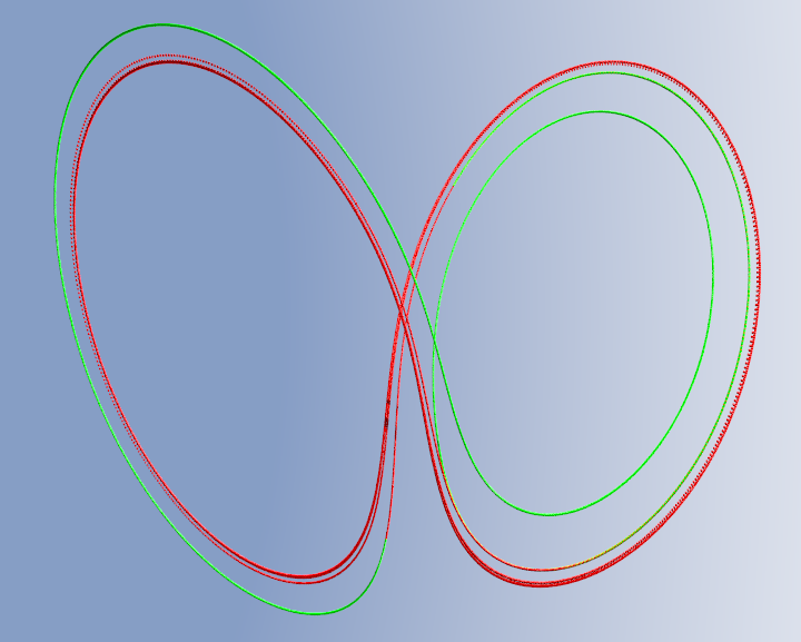
In Figure 7 we display the stable manifold of the orbit AB and the unstable manifold of ABB in Lorenz and observe several intersection of the two manifolds. The boundary of the unstable manifold crosses the stable manifold giving a connecting orbit. Let $P:[0,2L_{1}]\times[-1,1]\to\mathbb{R}^{3}$ denote the parameterization of the local stable manifold of the periodic orbit AB, whose period is $2L_{1}$ . Similarly, let $Q:[0,2L_{2}]\times[-1,1]\to\mathbb{R}^{3}$ be the parameterization of the unstable manifold of the periodic orbit ABB, whose period is given by $2L_{2}$ . Once the unstable manifold is restricted to one of its boundary circles only $3$ unknowns remain. We set $x=(\theta_{s},\sigma_{s},\theta_{u})$ so that the desired intersection is a zero of

S(x)=P(\theta_{s},\sigma_{s})-Q(\theta_{u},1).

Therefore $S:\mathbb{R}^{3}\to\mathbb{R}^{3}$ and it is possible to apply Newton’s method to obtain an approximation of the solution. Using this approach, we found

x\approx(1.942170529091222,0.000000560679355,1.253373698262391).

Then the connecting orbit can be computed from those coordinates in the parameter space. Since the value $\sigma_{s}$ of $x$ is already quite small we used the conjugacy relation (4) with $t=2$ and it is already sufficient. For the other half of the connecting orbit, we use (4) again to determine the “time of flight”. In this case, the unstable eigenvalue is $\lambda\approx 0.9947$ , so one would need to integrate backward in time for $t\approx 34.7246$ to obtain $\sigma$ smaller than $10^{-15}$ . Lets stress this point again: computing this orbit using the linear approximation of the stable/unstable manifolds would require almost $35$ units of time integration to cross from the unstable to the stable normal bundles. Using the parameterized manifolds no integration is necessary and the entire orbit is represented “locally”.

These results are displayed in figure 8. The green curve is the one obtained using the stable manifold while the trajectory in red correspond to the one using the unstable manifold and the time $t=34.7246$ .

4.2 The Circular Restricted Three Body Problem

The circular restricted three body problem (CRTBP) describes the evolution of a massless particle moving in the gravitational field of two other massive bodies, called the primaries. It is assumed that the primaries move in circular orbits about their center of mass. In this work we focus on the case that the third body moves in the plane of the primaries. In co-rotating coordinates the equations of motion are

\displaystyle\begin{cases}x^{\prime\prime}=2y^{\prime}+\frac{\partial H}{\partial x}\\ y^{\prime\prime}=-2x^{\prime}+\frac{\partial H}{\partial y}\end{cases}

(18)

with

H(x,y)=\frac{1}{2}(x^{2}+y^{2})+\frac{(1-\mu)}{\sqrt{(x+\mu)^{2}+y^{2}}}+\frac{\mu}{\sqrt{(x+\mu-1)^{2}+y^{2}}}.

Here $\mu$ is the mass ratio of the primary bodies. In the rotating frame:

1.

the center of mass is at the origin,
2.

the motion of the primaries is fixed and they sit on the $x-$ axis at $-\mu$ and $1-\mu$ .

This choice of coordinates introduces the Coriolis effect, that is the coordinates are non-inertial.

The CRTBP is much studied as an example in Hamiltonian dynamics and celestial mechanics going back to the work of Poincaré. It is a useful model of the motion of a satellite or astroid influenced by a two body system such as Earth/Moon, Sun/Earth, or Sun/Jupiter. It is also one of the simplest $N$ -body systems which admits chaotic motions, hence is not integrable. For further discussion of this and more general $N-$ body problems, we refer the reader to the books of Belbruno, [2004]; Belbruno, [2007]; Gómez et al., [2001]; Jorba and Masdemont, [1999]; Koon et al., [2000]; Meyer et al., [2009]. See also Alessi et al., [2009]; Belbruno et al., [2013]; Belbruno, [1981]; Canalias and Masdemont, [2006]; Font et al., [2009]; Gómez et al., [2004]; Koon et al., [2001]; Llibre et al., [1985]; Llibre and Simó, [1980]; Martínez and Simó, [2014]; Masdemont, [2005]. This list of references constitutes only the barest introduction to the relevant literature, but much more complete discussion is found in the books and papers just cited.

The system has five relative equilibrium points, also referred to as libration points, and we denote these by $\mathcal{L}_{j}$ with $j=1,2,3,4,5$ . Three of these lie on the $x$ -axis (the co-linear libration points). These are denoted $\mathcal{L}_{1,2,3}$ . See Figure 9 for a schematic representation of the problem.

Each of the co-linear libration points are of saddle $\times$ center stability type. By an application of the Lyapunov center theorem, each of the centers gives rise to one parameter families of periodic orbits. These are known as Lyapunov families. We compute invariant manifolds attached to some Lyapunov orbits below. First we transform to a polynomial problem.

Rewriting (18) as a vector field $\dot{u}=\hat{g}(u)$ gives

\hat{g}(u)=\begin{pmatrix}u^{2}\\ 2u^{4}+u^{1}-\frac{(1-\mu)(u^{1}+\mu)}{\sqrt{(u^{1}+\mu)^{2}+(u^{3})^{2}}^{3}}-\frac{\mu(u^{1}-1+\mu)}{\sqrt{(u^{1}-1+\mu)^{2}+(u^{3})^{2}}^{3}}\\ u^{4}\\ -2u^{2}+u^{3}-\frac{(1-\mu)u^{3}}{\sqrt{(u^{1}+\mu)^{2}+(u^{3})^{2}}^{3}}-\frac{\mu u^{3}}{\sqrt{(u^{1}-1+\mu)^{2}+(u^{3})^{2}}^{3}}\\ \end{pmatrix}.

(19)

This system is non-polynomial and we propose a related polynomial system through the use of automatic differentiation. Following Burgos-García et al., [2017]; Kepley and Mireles James, [2017]; Lessard et al., [2016] and the discussion in Section 2.3 we derive the polynomial vector field

g(v)=\begin{pmatrix}v^{2}\\ 2v^{4}+v^{1}-(1-\mu)(v^{1}+\mu)(v^{5})^{3}-\mu(v^{6})^{3}(v^{1}-1+\mu)\\ v^{4}\\ -2v^{2}+v^{3}-(1-\mu)v^{3}(v^{5})^{3}-\mu v^{3}(v^{6})^{3}\\ -(v^{5})^{3}((v^{1}+\mu)v^{2}+v^{3}v^{4})\\ -(v^{6})^{3}((v^{1}-1+\mu)v^{2}+v^{3}v^{4})\end{pmatrix},

(20)

with the additional (initial condition) constraints

	$\displaystyle v^{5}(0)$	$\displaystyle=\frac{1}{\sqrt{(v^{1}(0)+\mu)^{2}+(v^{3}(0))^{2}}}$
	$\displaystyle v^{6}(0)$	$\displaystyle=\frac{1}{\sqrt{(v^{1}(0)-1+\mu)^{2}+(v^{3}(0))^{2}}}.$

That is, we take $R$ defined by

R(u^{1},u^{2},u^{3},u^{4})=\left(\begin{array}[]{c}u^{1}\\ u^{2}\\ u^{3}\\ u^{4}\\ \frac{1}{\sqrt{(u^{1}+\mu)^{2}+(u^{3})^{2}}}\\ \frac{1}{\sqrt{(u^{1}-1+\mu)^{2}+(u^{3})^{2}}}\end{array}\right),\quad\quad\quad\mbox{and have}\quad DR(\mathbf{u})\hat{g}(\mathbf{u})=g(R(\mathbf{u})),

where $\mathbf{u}=(u^{1},u^{2},u^{3},u^{4})$ . Then the conjugacy of Equation (7) is satisfied. Moreover, one easily checks that $\pi_{4}(g(R(\mathbf{u})))=\hat{g}(\mathbf{u})$ . Of course $R$ is defined only on the complement of the collision set of the CRTBP.

Since periodic orbits in the CRTBP occur in one parameter families parameterized by energy, we fix $L$ and look for a periodic orbit with this half period. Moreover, we use the well known reversible symmetry of the problem to formulate a different boundary condition that will still provide periodic solutions. For example, orbits in a Lyapunov family of one of the co-linear libration points have no velocity in the $x$ direction when they cross the $x$ axis – and the time between the two crossing of the $x$ axis are separated by exactly the half orbit. So that a periodic solution $\gamma$ starting on the $x$ axis with frequency $2L$ will satisfy

\displaystyle\gamma_{2}(0)=0,\quad\gamma_{3}(0)=0,\quad\gamma_{2}\left(2L\right)=0\quad\mbox{and}\quad\gamma_{3}\left(2L\right)=0.

(21)

Remark 4.2.

Note that the last two conditions of (21) could also be $\gamma_{2}(L)=\gamma_{3}(L)=0$ . This would allow us to compute only the half orbit, the symmetry of the problem providing the solution for the second half of the trajectory. The use of Chebyshev expansion would allow such a choice. However, since the periodic orbit is not the final product of our computations, but only an input into the higher order equations we compute full orbits in this work.

For the remaining two conditions, we simply rewrite the initial condition on $v^{5}$ and $v^{6}$ after imposing the symmetry, so that

	$\displaystyle\gamma^{5}(0)=$	$\displaystyle\frac{1}{\|\gamma^{1}(0)+\mu\|},$
	$\displaystyle\gamma^{6}(0)=$	$\displaystyle\frac{1}{\|\gamma^{1}(0)-1+\mu\|}.$

Due to the choice of the boundary condition, time translation of the solution does not satisfy this system. Thus we drop the Poincaré condition previously given and obtain a system that is still fully determined and with isolated solutions (since we don’t solve for the period we dispense with one scalar equation). Two possibilities arise from that remark, one could fix $L$ to a given value and still find an orbit as previously mentioned. The other choice is to use $L$ as a variable and obtain a fully determined system by adding a condition in which the energy level is fixed to a chosen constant. Such a choice is necessary for example if we want to compute heteroclinic connecting orbits.

We summarize the discussion in the following lemma.

Lemma 4.3.

Let $v^{1}(t),v^{2}(t),v^{3}(t),v^{4}(t)$ be periodic function with same period $\omega$ and such that $\dot{v}^{1}=v^{2}$ , $\dot{v}^{3}=v^{4}$ . Let $v^{5}(t),v^{6}(t)$ satisfy

\displaystyle\begin{cases}\dot{v}^{5}(t)=-(v^{5}(t))^{3}((v^{1}(t)+\mu)v^{2}(t)+v^{3}(t)v^{4}(t)),&\\ v^{5}(0)=\frac{1}{\sqrt{(v^{1}(0)+\mu)^{2}+v^{3}(0)^{2}}},&\end{cases}

(22)

and

\displaystyle\begin{cases}\dot{v}^{6}(t)=-(v^{6}(t))^{3}((v^{1}(t)-1+\mu)v^{2}(t)+v^{3}(t)v^{4}(t)),&\\ v^{6}(0)=\frac{1}{\sqrt{(v^{1}(0)-1+\mu)^{2}+(v^{3}(0))^{2}}}.&\end{cases}

(23)

Then $v^{5}(t)$ and $v^{6}(t)$ are periodic with period $\omega$ .

Proof 4.4.

We first note that

w^{5}(t)=\frac{1}{\sqrt{(v^{1}(t)+\mu)^{2}+(v^{3}(t))^{2}}}

is a solution of (22). But by unicity of the solution it follows that $v^{5}(t)=w^{5}(t)$ . Moreover, we have that $w^{5}(t)$ is periodic with period $\omega$ since $v^{1}(t)$ and $v^{3}(t)$ are periodic with period $\omega$ . Thus $v^{5}(t)$ is periodic with period $\omega$ , as desired. For $v^{6}(t)$ , the proof is similar using the fact that

w^{6}(t)=\frac{1}{\sqrt{(v^{1}(t)-1+\mu)^{2}+(v^{3}(t))^{2}}}

is a solution of (23).

To fix the energy we have to use an integral of the CRTBP, namely

E(x,y,\dot{x},\dot{y})=x^{2}+y^{2}+2\frac{1-\mu}{\sqrt{(x+\mu)^{2}+y^{2}}}+2\frac{\mu}{\sqrt{(x-1+\mu)^{2}+y^{2}}}-(\dot{x}^{2}+\dot{y}^{2}),

known as the Jacobi integral. In our system of coordinates, this is

E(v^{1},v^{2},v^{3},v^{4},v^{5},v^{6}):=(v^{1})^{2}+(v^{3})^{2}+2(1-\mu)v^{5}+2\mu v^{6}-((v^{2})^{2}+(v^{4})^{2}).

Since $E$ is constant along any orbit of the system, we evaluate it at the endpoint of the first piece of the Chebyshev decomposition. This leads to a new phase condition that can replace the one previously exhibited at equation (16). In terms of the Chebyshev coefficients it is given by

	$\displaystyle f^{(0)}(A_{0})=$	$\displaystyle\left(a_{0,0}^{(1,1)}+2\displaystyle\sum_{k=1}^{\infty}a_{0,k}^{(1,1)}\right)^{2}+\left(a_{0,0}^{(1,3)}+2\displaystyle\sum_{k=1}^{\infty}a_{0,k}^{(1,3)}\right)^{2}+2(1-\mu)\left(a_{0,0}^{(1,5)}+2\displaystyle\sum_{k=1}^{\infty}a_{0,k}^{(1,5)}\right)$
		$\displaystyle+2\mu\left(a_{0,0}^{(1,6)}+2\displaystyle\sum_{k=1}^{\infty}a_{0,k}^{(1,6)}\right)-\left(a_{0,0}^{(1,2)}+2\displaystyle\sum_{k=1}^{\infty}a_{0,k}^{(1,2)}\right)^{2}-\left(a_{0,0}^{(1,4)}+2\displaystyle\sum_{k=1}^{\infty}a_{0,k}^{(1,4)}\right)^{2}.$		(24)

We now focus on expanding the operator we need to solve in order to obtain the coefficients of the Chebyshev expansion of the $i-$ th component of the solution. In the case $k\geq 1$ , each case is given by

	$\displaystyle f^{(i,1)}_{\alpha,k}(A_{\alpha})=2ka_{\alpha,k}^{(i,1)}-L_{i}\bigg($	$\displaystyle\alpha\lambda a_{\alpha,k\pm 1}^{(i,1)}-a_{\alpha,k\pm 1}^{(i,2)}\bigg),$
	$\displaystyle f^{(i,2)}_{\alpha,k}(A_{\alpha})=2ka_{\alpha,k}^{(i,2)}-L_{i}\bigg($	$\displaystyle\alpha\lambda a_{\alpha,k\pm 1}^{(i,2)}-a_{\alpha,k\pm 1}^{(i,1)}-2a_{\alpha,k\pm 1}^{(i,4)}+(1-\mu)\mathcal{C}_{\alpha,k\pm 1}^{(i)}(1,5,5,5)+\mu\mathcal{C}_{\alpha,k\pm 1}^{(i)}(1,6,6,6)$
		$\displaystyle+(\mu-\mu^{2})\mathcal{C}_{\alpha,k\pm 1}^{(i)}(5,5,5)+(\mu^{2}-\mu)\mathcal{C}_{\alpha,k\pm 1}^{(i)}(6,6,6)\bigg),$
	$\displaystyle f^{(i,3)}_{\alpha,k}(A_{\alpha})=2ka_{\alpha,k}^{(i,3)}-L_{i}\bigg($	$\displaystyle\alpha\lambda a_{\alpha,k\pm 1}^{(i,3)}-a_{\alpha,k\pm 1}^{(i,4)}\bigg),$
	$\displaystyle f^{(i,4)}_{\alpha,k}(A_{\alpha})=2ka_{\alpha,k}^{(i,4)}-L_{i}\bigg($	$\displaystyle\alpha\lambda a_{\alpha,k\pm 1}^{(i,4)}+2a_{\alpha,k\pm 1}^{(i,2)}-a_{\alpha,k\pm 1}^{(i,3)}+(1-\mu)\mathcal{C}_{\alpha,k\pm 1}^{(i)}(3,5,5,5)+\mu\mathcal{C}_{\alpha,k\pm 1}^{(i)}(3,6,6,6)\bigg),$
	$\displaystyle f^{(i,5)}_{\alpha,k}(A_{\alpha})=2ka_{\alpha,k}^{(i,5)}-L_{i}\bigg($	$\displaystyle\alpha\lambda a_{1,k\pm 1}^{(i,5)}+\mathcal{C}_{\alpha,k\pm 1}^{(i)}(1,2,5,5,5)+\mu\mathcal{C}_{\alpha,k\pm 1}^{(i)}(2,5,5,5)+\mathcal{C}_{\alpha,k\pm 1}^{(i)}(3,4,5,5,5)\bigg),$
	$\displaystyle f^{(i,6)}_{\alpha,k}(A_{\alpha})=2ka_{\alpha,k}^{(i,6)}-L_{i}\bigg($	$\displaystyle\alpha\lambda a_{1,k\pm 1}^{(i,6)}+\mathcal{C}_{\alpha,k\pm 1}^{(i)}(1,2,6,6,6)+(\mu-1)\mathcal{C}_{\alpha,k\pm 1}^{(i)}(2,6,6,6)+\mathcal{C}_{\alpha,k\pm 1}^{(i)}(3,4,6,6,6)\bigg).$

The cases $k=0$ are as given in (13) for every $i=2,\ldots,D$ . In the case $i=1$ , for the periodic orbit we use the condition previously given to rewrite the problem as a zero finding of an operator. Those are given by

	$\displaystyle f^{(1,1)}_{0,0}(A_{\alpha})$	$\displaystyle=a_{0,0}^{(D,2)}+2\displaystyle\sum_{k=1}^{\infty}a_{0,k}^{(D,2)}(-1)^{k},$
	$\displaystyle f^{(1,2)}_{0,0}(A_{\alpha})$	$\displaystyle=a_{0,0}^{(D,3)}+2\displaystyle\sum_{k=1}^{\infty}a_{0,k}^{(D,3)}(-1)^{k},$
	$\displaystyle f^{(1,3)}_{0,0}(A_{\alpha})$	$\displaystyle=a_{0,0}^{(1,2)}+2\displaystyle\sum_{k=1}^{\infty}a_{0,k}^{(1,2)},$
	$\displaystyle f^{(1,4)}_{0,0}(A_{\alpha})$	$\displaystyle=a_{0,0}^{(1,3)}+2\displaystyle\sum_{k=1}^{\infty}a_{0,k}^{(1,3)},$
	$\displaystyle f^{(1,5)}_{0,0}(A_{\alpha})$	$\displaystyle=\left(a_{0,0}^{(1,5)}+2\displaystyle\sum_{k=1}^{\infty}a_{0,k}^{(1,5)}(-1)^{k}\right)\left\|a_{0,0}^{(1,1)}+2\displaystyle\sum_{k=1}^{\infty}a_{0,k}^{(1,1)}(-1)^{k}+\mu\right\|-1,$
	$\displaystyle f^{(1,6)}_{0,0}(A_{\alpha})$	$\displaystyle=\left(a_{0,0}^{(1,6)}+2\displaystyle\sum_{k=1}^{\infty}a_{0,k}^{(1,5)}(-1)^{k}\right)\left\|a_{0,0}^{(1,1)}+2\displaystyle\sum_{k=1}^{\infty}a_{0,k}^{(1,1)}(-1)^{k}-1+\mu\right\|-1.$

The operator is now completely determined. In order to approximate the solution we truncate the unknowns and the operator a similar way as for the Lorenz system and obtain an operator such that $F:\mathbb{R}^{6mD+1}\to\mathbb{R}^{6mD+1}$ in the case $\alpha=0,1$ and such that $F:\mathbb{R}^{6mD}\to\mathbb{R}^{6mD}$ in the higher dimensional cases. Again, only the search for the periodic orbit requires a good initial guess to obtain the approximation. Following Lessard et al., [2016] we get an initial guess on which we applied Newton’s method. To present results, we regrouped different orbits with the same level of energy.

Figure 10 illustrates two Lyapunov periodic orbits associated with the libration points $\mathcal{L}_{1}$ and $\mathcal{L}_{2}$ . Both orbit have energy $E=3.17$ and have been computed using $m=50$ Chebyshev nodes and $D=8$ Chebyshev domains. The periods are $L\approx 1.7122$ for the orbit around $\mathcal{L}_{2}$ and $L\approx 1.4242$ for the orbit around $\mathcal{L}_{1}$ . See Figure 11 for an illustration of the numerically computed parameterized invariant manifolds.

We must stress that these computations were preformed for the polynomial equation $\dot{v}=g(v(t))$ , where $g$ is given by (20). To show that a point laying in an invariant manifolds in the polynomial problem corresponds to a point on the manifold for the original CRTBP we use the following Theorem. Intuitively this works because of the conjugacy described in Equation (7).

Theorem 4.5.

Let $P(t,\sigma)$ be a parameterization of the local stable manifold of a given periodic orbit $v(t)$ satisfying $\dot{v}=g(v(t))$ , where $g$ is given by (20). If $x_{0}\in\mathbb{R}^{6}$ is such that $x_{0}=P(t_{0},\sigma_{0})$ , then the point $y_{0}\in\mathbb{R}^{4}$ given by the first four component of $x_{0}$ is in the stable set of the corresponding periodic orbit of $\dot{u}=f(u)$ , where $f$ is given by (19).

Proof 4.6.

Note that using the same remark as in the proof of Lemma (4.3), we obtain from the periodic orbit $v(t)$ a periodic orbit of the CRTBP. That is a periodic solution of $\dot{u}=f(u(t))$ . We denote this orbit by $u(t)$ and we have that $v^{i}(t)=u^{i}(t)$ for $i=1,2,3,4$ , while

v^{5}(t)=\frac{1}{\sqrt{(u^{1}(t)+\mu)^{2}+u^{3}(t)^{2}}}~\mbox{and}~v^{6}(t)=\frac{1}{\sqrt{(u^{1}(t)-1+\mu)^{2}+u^{3}(t)^{2}}}.

Let $x(t)$ denote the trajectory obtained by flowing $x_{0}$ forward in time by $\Phi(v,t)$ the flow solution of $\dot{v}=g(v(t))$ . So that, using the conjugacy relation (4), we have

x(t)=P(t_{0}+t,e^{\lambda t}\sigma_{0}),

where $\lambda$ is the stable eigenvalue associated to the orbit. Moreover, it follows that

	$\displaystyle\dot{x}(t)$	$\displaystyle=\frac{\partial}{\partial t}P(t_{0}+t,e^{\lambda t}\sigma_{0})$
		$\displaystyle=\frac{\partial}{\partial t}\Phi(x_{0},t)$
		$\displaystyle=g(x(t)).$

Thus, by definition of $g$

x^{5}(t)=\frac{1}{\sqrt{(x^{1}(t)+\mu)^{2}+(x^{3}(t))^{2}}}+C_{1}

and

x^{6}(t)=\frac{1}{\sqrt{(x^{1}(t)-1+\mu)^{2}+(x^{3}(t))^{2}}}+C_{2}.

Here $C_{1},C_{2}$ are arbitrary constants. But $x_{0}\in W^{s}(v)$ , so that for any $\epsilon>0$ there exists $T$ such that for all $t\geq T$ , we have that

\min_{s\in[0,\omega]}\left|x^{5}(t)-v^{5}(s)\right|<\epsilon.

This force $C_{1}=0$ . Similarly, we have that $C_{2}=0$ . Now $x^{5}$ and $x^{6}$ in $g$ are rewritten with the first four component so that $g$ reduce to $f$ and $y(t)=(x^{1}(t),x^{2}(t),x^{3}(t),x^{4}(t))$ satisfies $\dot{y}(t)=f(y(t))$ . Moreover, since $x_{0}\in W^{s}(v)$ , we have that $y(t)$ is in the stable set of the corresponding orbit $u(t)$ , as desired.

4.2.1 Connecting orbits as solutions of boundary value problems

As in Section 4.1.1 we now use the parametrized manifolds to compute connecting orbits between period orbits. In the present section we consider heteroclinic orbits for the CRTBP and we do not find any short connections. Instead, we solve a two point boundary value problem with the manifolds as boundary conditions. This strategy is standard and is for example discussed in detail in Doedel and Friedman, [1989]; Friedman and Doedel, [1993]; Doedel et al., [2008]; Doedel et al., [2009].

The references just cited obtain boundary conditions by projecting onto the linear approximation of the stable/unstable manifolds given by the stable/unstable normal bundles associated with the periodic orbit. Projecting instead onto high order parameterizations can substantially reduce the integration time and numerically stabilize the problem. The behavior of the connecting orbit on the manifold is then recovered via the flow conjugacy.

Remark 4.7.

In this work we compute connecting orbits by numerically integrating the system. However, one could adapt the approach developed in section 3 with $\alpha=0$ to compute any orbit solution of a given boundary value problem expanded as Chebyshev series. This has been done in Lessard and Reinhardt, [2014]; van den Berg et al., [2015]; van den Berg and Sheombarsing, [2016] and even leads to computer assisted proofs. We return to this remark in an upcoming work. We also refer to Arioli, [2002]; Arioli, [2004]; Capiński, [2012]; Wilczak and Zgliczyński, [2003] for further reading about computer assisted proofs in the CRTBP.

We let $P$ and $Q$ denote parameterizations of the stable and unstable manifolds, and seek $(\theta_{u},\sigma_{u})$ , $(\theta_{s},\sigma_{s})$ and an integrating time $T$ – or “time of flight” – such that

\displaystyle\Phi(P_{0},T)

\displaystyle=P(\theta_{s},\sigma_{s}),

(25)

where $P_{0}=Q(\theta_{u},\sigma_{u})$ . Equation (25) has five unknowns, namely the integrating time and the parameters on both manifold. Since orbits of the CRTBP lie in $\mathbb{R}^{4}$ , Equation (25) provides only four equations and we have more unknowns than equations. As a result we cannot expect to isolate a solution. To remedy the situation we simply fix $\sigma_{u}=-1$ , removing one of the variables. This corresponds to a choice of boundary components for the local unstable manifold.

Remark 4.8.

Recall that the energy is constant along solution curves, and it’s impossible to find a connecting orbit between two periodic solution with different energy level. We avoided this problem by introducing the energy as the phase condition when we solve for the underlying orbit. Recall the definition of $f^{(0)}$ in (24).

Using Newton’s method with the unstable manifold of the orbit on the right in figure 10 and the stable manifold of the orbit on the left we found an approximation of a solution to this problem where

	$\displaystyle(\theta_{u},\sigma_{u})$	$\displaystyle\approx(3.086681925168687,-1)$
	$\displaystyle(\theta_{s},\sigma_{s})$	$\displaystyle\approx(0.065696587097979,1)$
	$\displaystyle T$	$\displaystyle\approx 1.654424821513812.$

Both manifolds were computed with $m=50$ , $D=8$ , $N=50$ , $K=5$ and $k_{0}=10$ . To find an initial guess on which to apply Newton’s method we integrated $40$ points evenly distributed on the boundary of the unstable manifold and observed that some orbits were potentially intersecting the stable manifold. The connecting orbit and the two manifold are displayed in figure 12.

We also use the conjugacy relation to extend the connecting orbit forward and backward on the manifolds. Integrating in the parameter space until $\sigma_{s}\approx 10^{-15}$ takes

t\approx 12.3688,

and for the backward trajectory

t\approx 16.1050.

The full trajectory is displayed in figure 13. Note that out of the three pieces of the trajectory, only the one in blue was obtained by numerically integrating the system and this piece required a time step of only $2$ time units. Redoing the computation but projecting onto the linear approximations would result in a time of flight of roughly $30$ time units.

4.3 A Circular Restricted Four Body Problem

We now consider a gravitational problem consisting of three massive bodies (again called the primaries) located at the vertices of an equilateral triangle in the central configuration of Lagrange. These bodies rotate in circular orbits about their common center of mass, all with the same period, rigidly fixing the triangular formation. After changing to a co-rotating frame we are interested the motion of a massless fourth particle moving in the gravitational field of the primaries. In the present work we suppose that the massless particle moves in the plane of the primaries.

It is standard practice to normalize the masses of the primaries so that $0<m_{3}\leq m_{2}\leq m_{1}$ , and

m_{1}+m_{2}+m_{3}=1.

The rotating coordinates are chosen so that the center of mass is at the origin, the largest primary is on the $x$ -axis, the $x$ -axis cuts the side of the triangle opposite the largest primary, and the smallest primary is in the first quadrant. More explicitly, the primaries are located at positions

p_{1}=(x_{1},y_{1},z_{1}),\quad\quad p_{2}=(x_{2},y_{2},z_{2}),\quad\quad\text{and}\quad\quad p_{3}=(x_{3},y_{3},z_{3}),

with

$\displaystyle x_{1}$	$\displaystyle=$	$\displaystyle\frac{-\|K\|\sqrt{m_{2}^{2}+m_{2}m_{3}+m_{3}^{2}}}{K}$
$\displaystyle y_{1}$	$\displaystyle=$	$\displaystyle 0$
$\displaystyle z_{1}$	$\displaystyle=$	$\displaystyle 0$

$\displaystyle x_{2}$	$\displaystyle=$	$\displaystyle\frac{\|K\|\left[(m_{2}-m_{3})m_{3}+m_{1}(2m_{2}+m_{3})\right]}{2K\sqrt{m_{2}^{2}+m_{2}m_{3}+m_{3}^{2}}}$
$\displaystyle y_{2}$	$\displaystyle=$	$\displaystyle\frac{-\sqrt{3}m_{3}}{2m_{2}^{3/2}}\sqrt{\frac{m_{2}^{3}}{m_{2}^{2}+m_{2}m_{3}+m_{3}^{2}}}$
$\displaystyle z_{2}$	$\displaystyle=$	$\displaystyle 0$

and

$\displaystyle x_{3}$	$\displaystyle=$	$\displaystyle\frac{\|K\|}{2\sqrt{m_{2}^{2}+m_{2}m_{3}+m_{3}^{2}}}$
$\displaystyle y_{3}$	$\displaystyle=$	$\displaystyle\frac{\sqrt{3}}{2\sqrt{m_{2}}}\sqrt{\frac{m_{2}^{3}}{m_{2}^{2}+m_{2}m_{3}+m_{3}^{2}}}$
$\displaystyle z_{3}$	$\displaystyle=$	$\displaystyle 0$

where

K=m_{2}(m_{3}-m_{2})+m_{1}(m_{2}+2m_{3}).

Define the potential function

\Omega(x,y,z):=\frac{1}{2}(x^{2}+y^{2})+\frac{m_{1}}{r_{1}(x,y,z)}+\frac{m_{2}}{r_{2}(x,y,z)}+\frac{m_{3}}{r_{3}(x,y,z)},

with

r_{1}(x,y,z):=\sqrt{(x-x_{1})^{2}+(y-y_{1})^{2}+(z-z_{1})^{2}},

r_{2}(x,y,z):=\sqrt{(x-x_{2})^{2}+(y-y_{2})^{2}+(z-z_{2})^{2}},

and

r_{3}(x,y,z):=\sqrt{(x-x_{3})^{2}+(y-y_{3})^{2}+(z-z_{3})^{2}}.

The equations of motion for the massless particle in the co-rotating coordinates are

\begin{split}\ddot{x}-2\dot{y}&=\Omega_{x},\\ \ddot{y}+2\dot{x}&=\Omega_{y},\\ \ddot{z}&=\Omega_{z},\end{split}

(26)

where

\frac{\partial}{\partial x}\Omega=\Omega_{x}(x,y,z)=x-\frac{m_{1}(x-x_{1})}{r_{1}(x,y,z)^{3}}-\frac{m_{2}(x-x_{2})}{r_{2}(x,y,z)^{3}}-\frac{m_{3}(x-x_{3})}{r_{3}(x,y,z)^{3}},

\frac{\partial}{\partial y}\Omega=\Omega_{y}(x,y,z)=y-\frac{m_{1}(y-y_{1})}{r_{1}(x,y,z)^{3}}-\frac{m_{2}(y-y_{2})}{r_{2}(x,y,z)^{3}}-\frac{m_{3}(y-y_{3})}{r_{3}(x,y,z)^{3}},

and

\frac{\partial}{\partial z}\Omega=\Omega_{z}(x,y,z)=-\frac{m_{1}(z-z_{1})}{r_{1}(x,y,z)^{3}}-\frac{m_{2}(z-z_{2})}{r_{2}(x,y,z)^{3}}-\frac{m_{3}(z-z_{3})}{r_{3}(x,y,z)^{3}}.

The problem is the subject of many studies beginning with the work of Simó, [1978]. Detailed analysis of the equilibrium solutions and their stability are found in Barros and Leandro, [2014]; Leandro, [2006]; Baltagiannis and Papadakis, 2011b []; Rusu and Santoprete, [2016]; Alvarez-Ramírez and Delgado, [2003], while periodic orbits are studied in Papadakis, 2016a []; Baltagiannis and Papadakis, 2011a []; Papadakis, 2016b []; Burgos-García and Delgado, [2013]; Burgos-García et al., [2017]. The earlier study of Blazevski and Ocampo, [2012] considers stable/unstable manifolds attached to periodic orbits (using the linear approximation given by the stable/unstable normal bundles combined with numerical integration). More complex dynamical behavior such as heteroclinic/homoclinic phenomena and transport are studied numerically in Alvarez-Ramírez and Barrabés, [2015]; Álvarez-Ramírez and Vidal, [2009]; Gidea and Burgos, [2003]; Kepley and Mireles James, [2017]. A Hill’s approximation is derived in Burgos-García and Gidea, [2015]. See also the more theoretical studies of Cheng and She, [2015]; Cheng and She, [2017]; She and Cheng, [2014].

The CRFBP has $8,9$ , or $10$ equilibrium points depending on the values of the mass parameters. These will have either center $\times$ center, center $\times$ saddle, or saddle-focus stability, depending on the ratios of the masses. As in the CRTBP, the center $\times$ saddle equilibria give rise to one parameter families of hyperbolic Lyapunov orbits. We compute local stable/unstable manifolds attached to one of these below.

Using automatic differentiation we derive a related polynomial vector field

\displaystyle g(v)=\begin{pmatrix}v^{2}\\ 2v^{4}+v^{1}-m_{1}v^{1}(v^{7})^{3}-m_{2}v^{1}(v^{8})^{3}-m_{3}v^{1}(v^{9})^{3}+m_{1}x_{1}(v^{7})^{3}+m_{2}x_{2}(v^{8})^{3}+m_{3}x_{3}(v^{9})^{3}+\beta v^{2}\\ v^{4}\\ -2v^{2}+v^{3}-m_{1}v^{3}(v^{7})^{3}-m_{2}v^{3}(v^{8})^{3}-m_{3}v^{3}(v^{9})^{3}+m_{1}y_{1}(v^{7})^{3}+m_{2}y_{2}(v^{8})^{3}+m_{3}y_{3}(v^{9})^{3}\\ v^{6}\\ -m_{1}v^{5}(v^{7})^{3}-m_{2}v^{5}(v^{8})^{3}-m_{3}v^{5}(v^{9})^{3}+m_{1}z_{1}(v^{7})^{3}+m_{2}z_{2}(v^{8})^{3}+m_{3}z_{3}(v^{9})^{3}\\ -v^{1}v^{2}(v^{7})^{3}-v^{3}v^{4}(v^{7})^{3}-v^{5}v^{6}(v^{7})^{3}+x_{1}v^{2}(v^{7})^{3}+y_{1}v^{4}(v^{7})^{3}+z_{1}v^{6}(v^{7})^{3}+\alpha_{1}(v^{7})^{3}\\ -v^{1}v^{2}(v^{8})^{3}-v^{3}v^{4}(v^{8})^{3}-v^{5}v^{6}(v^{8})^{3}+x_{2}v^{2}(v^{8})^{3}+y_{2}v^{4}(v^{8})^{3}+z_{2}v^{6}(v^{8})^{3}+\alpha_{2}(v^{8})^{3}\\ -v^{1}v^{2}(v^{9})^{3}-v^{3}v^{4}(v^{9})^{3}-v^{5}v^{6}(v^{9})^{3}+x_{3}v^{2}(v^{9})^{3}+y_{3}v^{4}(v^{9})^{3}+z_{3}v^{6}(v^{9})^{3}+\alpha_{3}(v^{9})^{3}\end{pmatrix}.

The mapping $R$ used in the automatic differentiation is defined Kepley and Mireles James, [2017], but is similar to the mapping discussed above for the three body case.

The constants terms $\beta,\alpha_{1},\alpha_{2},\alpha_{3}$ are Lagrange multipliers, which are needed to isolate a periodic solution (this time we will not impose any symmetry, hence the boundary condition constraints remain and have to be balanced). The following result, whose proof is found in Burgos-García et al., [2017], explains the relation between the polynomial and non-polynomial problems.

Lemma 4.9.

Assume that $\beta,\alpha_{1},\alpha_{2},\alpha_{3},L\in\mathbb{R}$ are fixed constant with $L>0$ and let $\textbf{n},\textbf{p}\in\mathbb{R}^{6}$ be fixed vector. Suppose that $u:[0,2L]\to\mathbb{R}^{9}$ is a periodic solution of $\dot{v}(t)=g(v)$ with $g$ as above and

	$\displaystyle 0$	$\displaystyle=\textbf{n}\cdot((u^{1}(0),u^{2}(0),u^{3}(0),u^{4}(0),u^{5}(0),u^{6}(0))^{T}-\textbf{p})$
	$\displaystyle u^{7}(0)$	$\displaystyle=\frac{1}{\sqrt{(u^{1}(0)-x_{1})^{2}+(u^{3}(0)-y_{1})^{2}+(u^{5}(0)-z_{1})^{2}}}$
	$\displaystyle u^{8}(0)$	$\displaystyle=\frac{1}{\sqrt{(u^{1}(0)-x_{2})^{2}+(u^{3}(0)-y_{2})^{2}+(u^{5}(0)-z_{2})^{2}}}$
	$\displaystyle u^{9}(0)$	$\displaystyle=\frac{1}{\sqrt{(u^{1}(0)-x_{3})^{2}+(u^{3}(0)-y_{3})^{2}+(u^{5}(0)-z_{3})^{2}}}$

and that $u^{7}(t),u^{8}(t),u^{9}(t)>0$ for all $t\in[0,2L]$ . Then

1.

$\beta=\alpha_{1}=\alpha_{2}=\alpha_{3}=0$
2.

the function $\hat{u}:[0,2L]\to\mathbb{R}^{6}$ given by

$\hat{u}(t)=(u^{1}(0),u^{2}(0),u^{3}(0),u^{4}(0),u^{5}(0),u^{6}(0))^{T}$

is a periodic solution of the four body problem.

Yet, the variables $\alpha_{1},\alpha_{2},\alpha_{3}$ are not necessary in the Chebyshev setting since one can use the following lemma to force the initial value condition on $v^{7},v^{8},v^{9}$ without introducing additional equations. The proof is omitted since it is similar to the proof of Lemma 4.3.

Lemma 4.10.

Let $v^{1}(t),v^{2}(t),v^{3}(t),v^{4}(t),v^{5}(t),v^{6}(t)$ be periodic solution with same period $\omega$ and such that $\dot{v}^{1}=v^{2}$ , $\dot{v}^{3}=v^{4}$ , $\dot{v}^{5}=v^{6}$ . Let $v^{7}(t),v^{8}(t),v^{9}(t)$ satisfy

	$\displaystyle\dot{v}^{7}(t)$	$\displaystyle=-(v^{7}(t))^{3}\left((v^{1}(t)-x_{1})v^{2}(t)+(v^{3}(t)-y_{1})v^{4}(t)+(v^{5}(t)-z_{1})v^{6}(t)\right)$
	$\displaystyle v^{7}(0)$	$\displaystyle=\frac{1}{\sqrt{(v^{1}(0)-x_{1})^{2}+(v^{3}(0)-y_{1})^{2}+(v^{5}(0)-z_{1})^{2}}}$
	$\displaystyle\dot{v}^{8}(t)$	$\displaystyle=-(v^{8}(t))^{3}\left((v^{1}(t)-x_{2})v^{2}(t)+(v^{3}(t)-y_{2})v^{4}(t)+(v^{5}(t)-z_{2})v^{6}(t)\right)$
	$\displaystyle v^{8}(0)$	$\displaystyle=\frac{1}{\sqrt{(v^{1}(0)-x_{2})^{2}+(v^{3}(0)-y_{2})^{2}+(v^{5}(0)-z_{2})^{2}}}$
	$\displaystyle\dot{v}^{9}(t)$	$\displaystyle=-(v^{9}(t))^{3}\left((v^{1}(t)-x_{3})v^{2}(t)+(v^{3}(t)-y_{3})v^{4}(t)+(v^{5}(t)-z_{3})v^{6}(t)\right)$
	$\displaystyle v^{9}(0)$	$\displaystyle=\frac{1}{\sqrt{(v^{1}(0)-x_{3})^{2}+(v^{3}(0)-y_{3})^{2}+(v^{5}(0)-z_{3})^{2}}}.$

Then $v^{7}(t),v^{8}(t)$ and $v^{9}(t)$ are periodic with period $\omega$ .

The extra condition balancing the system is the Poincaré condition which rewrites exactly as in (16). This condition rejects potential time translation of a periodic solution. The other conditions are coming from automatic differentiation and are given by

	$\displaystyle v^{7}(0)^{2}\big((v^{1}(0)-x_{1})^{2}+(v^{3}(0)-y_{1})^{2}+(v^{5}(0)-z_{1})^{2}\big)-1=0,$
	$\displaystyle v^{8}(0)^{2}\big((v^{1}(0)-x_{2})^{2}+(v^{3}(0)-y_{2})^{2}+(v^{5}(0)-z_{2})^{2}\big)-1=0,$
	$\displaystyle v^{9}(0)^{2}\big((v^{1}(0)-x_{3})^{2}+(v^{3}(0)-y_{3})^{2}+(v^{5}(0)-z_{3})^{2}\big)-1=0.$

The boundary condition for each Chebyshev subdomain being used for this problem define the operators $f^{(i,j)}_{\alpha,0}$ as previously given in (13) and (14). For all $1\leq i\leq D$ , the case for $k\geq 1$ are given by

	$\displaystyle f^{(i,1)}_{\alpha,k}(A)=2ka_{\alpha,k}^{(i,1)}+L_{i}\bigg($	$\displaystyle-\alpha\lambda a_{\alpha,k\pm 1}^{(i,1)}+a_{\alpha,k\pm 1}^{(i,2)}\bigg),$
	$\displaystyle f^{(i,2)}_{\alpha,k}(A)=2ka_{\alpha,k}^{(i,2)}+L_{i}\bigg($	$\displaystyle-\alpha\lambda a_{\alpha,k\pm 1}^{(i,2)}+2a_{\alpha,k\pm 1}^{(i,4)}+a_{\alpha,k\pm 1}^{(i,1)}+\beta a_{\alpha,k\pm 1}^{(i,2)}$
		$\displaystyle-m_{1}\mathcal{C}_{\alpha,k\pm 1}^{(i)}(1,7,7,7)-m_{2}\mathcal{C}_{\alpha,k\pm 1}^{(i)}(1,8,8,8)-m_{3}\mathcal{C}_{\alpha,k\pm 1}^{(i)}(1,9,9,9)$
		$\displaystyle+m_{1}x_{1}\mathcal{C}_{\alpha,k\pm 1}^{(i)}(7,7,7)+m_{2}x_{2}\mathcal{C}_{\alpha,k\pm 1}^{(i)}(8,8,8)+m_{3}x_{3}\mathcal{C}_{\alpha,k\pm 1}^{(i)}(9,9,9)\bigg),$

	$\displaystyle f^{(i,3)}_{\alpha,k}(A)=2ka_{\alpha,k}^{(i,3)}+L_{i}\bigg($	$\displaystyle-\alpha\lambda a_{\alpha,k\pm 1}^{(i,3)}+a_{\alpha,k\pm 1}^{(i,4)}\bigg),$
	$\displaystyle f^{(i,4)}_{\alpha,k}(A)=2ka_{\alpha,k}^{(i,4)}+L_{i}\bigg($	$\displaystyle-\alpha\lambda a_{\alpha,k\pm 1}^{(i,4)}-2a_{\alpha,k\pm 1}^{(i,2)}+a_{\alpha,k\pm 1}^{(i,3)}$
		$\displaystyle-m_{1}\mathcal{C}_{\alpha,k\pm 1}^{(i)}(3,7,7,7)-m_{2}\mathcal{C}_{\alpha,k\pm 1}^{(i)}(3,8,8,8)-m_{3}\mathcal{C}_{\alpha,k\pm 1}^{(i)}(3,9,9,9)$
		$\displaystyle+m_{1}y_{1}\mathcal{C}_{\alpha,k\pm 1}^{(i)}(7,7,7)+m_{2}y_{2}\mathcal{C}_{\alpha,k\pm 1}^{(i)}(8,8,8)+m_{3}y_{3}\mathcal{C}_{\alpha,k\pm 1}^{(i)}(9,9,9)\bigg),$

	$\displaystyle f^{(i,5)}_{\alpha,k}(A)=2ka_{\alpha,k}^{(i,5)}+L_{i}\bigg($	$\displaystyle-\alpha\lambda a_{\alpha,k\pm 1}^{(i,5)}+a_{\alpha,k\pm 1}^{(i,6)}\bigg),$
	$\displaystyle f^{(i,6)}_{\alpha,k}(A)=2ka_{\alpha,k}^{(i,6)}+L_{i}\bigg($	$\displaystyle-\alpha\lambda a_{\alpha,k\pm 1}^{(i,6)}-m_{1}\mathcal{C}_{\alpha,k\pm 1}^{(i)}(5,7,7,7)-m_{2}\mathcal{C}_{\alpha,k\pm 1}^{(i)}(5,8,8,8)-m_{3}\mathcal{C}_{\alpha,k\pm 1}^{(i)}(5,9,9,9)$
		$\displaystyle+m_{1}z_{1}\mathcal{C}_{\alpha,k\pm 1}^{(i)}(7,7,7)+m_{2}z_{2}\mathcal{C}_{\alpha,k\pm 1}^{(i)}(8,8,8)+m_{3}z_{3}\mathcal{C}_{\alpha,k\pm 1}^{(i)}(9,9,9)\bigg),$

	$\displaystyle f^{(i,7)}_{\alpha,k}(A)=2ka_{\alpha,k}^{(i,7)}+L_{i}\bigg($	$\displaystyle-\alpha\lambda a_{\alpha,k\pm 1}^{(i,7)}-\mathcal{C}_{\alpha,k\pm 1}^{(i)}(1,2,7,7,7)-\mathcal{C}_{\alpha,k\pm 1}^{(i)}(3,4,7,7,7)-\mathcal{C}_{\alpha,k\pm 1}^{(i)}(5,6,7,7,7)$
		$\displaystyle+x_{1}\mathcal{C}_{\alpha,k\pm 1}^{(i)}(2,7,7,7)+y_{1}\mathcal{C}_{\alpha,k\pm 1}^{(i)}(4,7,7,7)+z_{1}\mathcal{C}_{\alpha,k\pm 1}^{(i)}(6,7,7,7)\bigg),$

	$\displaystyle f^{(i,8)}_{\alpha,k}(A)=2ka_{\alpha,k}^{(i,8)}+L_{i}\bigg($	$\displaystyle-\alpha\lambda a_{\alpha,k\pm 1}^{(i,8)}-\mathcal{C}_{\alpha,k\pm 1}^{(i)}(1,2,8,8,8)-\mathcal{C}_{\alpha,k\pm 1}^{(i)}(3,4,8,8,8)-\mathcal{C}_{\alpha,k\pm 1}^{(i)}(5,6,8,8,8)$
		$\displaystyle+x_{2}\mathcal{C}_{\alpha,k\pm 1}^{(i)}(2,8,8,8)+y_{2}\mathcal{C}_{\alpha,k\pm 1}^{(i)}(4,8,8,8)+z_{2}\mathcal{C}_{\alpha,k\pm 1}^{(i)}(6,8,8,8)\bigg),$

	$\displaystyle f^{(i,9)}_{\alpha,k}(A)=2ka_{\alpha,k}^{(i,9)}+L_{i}\bigg($	$\displaystyle-\alpha\lambda a_{\alpha,k\pm 1}^{(i,9)}-\mathcal{C}_{\alpha,k\pm 1}^{(i)}(1,2,9,9,9)-\mathcal{C}_{\alpha,k\pm 1}^{(i)}(3,4,9,9,9)-\mathcal{C}_{\alpha,k\pm 1}^{(i)}(5,6,9,9,9)$
		$\displaystyle+x_{3}\mathcal{C}_{\alpha,k\pm 1}^{(i)}(2,9,9,9)+y_{3}\mathcal{C}_{\alpha,k\pm 1}^{(i)}(4,9,9,9)+z_{3}\mathcal{C}_{\alpha,k\pm 1}^{(i)}(6,9,9,9)\bigg),$

Again, we solve recursively the truncated operator to obtain an approximation of the manifold. The case $\alpha=0$ will have the extra variable $\beta$ from Lemma (4.9) and the case $\alpha=1$ will have the eigenvalue as an extra unknown. Note that in this case we fix the frequency $L$ to a constant, it is still possible to find a solution for the same reason as mentioned in the case of the CRTBP. In figure 15, we display an unstable manifold for a planar Lyapunov orbit about $\mathcal{L}_{8}$ . The computations were done with $D=4$ and $N=60$ . We used masses

m_{1}\approx 0.9987,~m_{2}\approx 0.0010~\mbox{and}~m_{3}\approx 0.0003.

We remark that, for the purposes of the present demonstration, we could have taken $m_{1},m_{2},m_{3}$ to have more or less any values. Nevertheless the particular choice of mass values was suggested in Burgos-García, [2017]. The values of $m_{1},m_{2}$ correspond respectively to the mass of the primary star in the binary system Epsilon Reticuli (Henry Draper Catalogue number $27442$ ), and the mass of an extra solar planet discovered orbiting HD $27442$ in the year $2000$ . The mass ratio of these bodies is such that the system could form a CRFBP with a third trojan object. Our value of $m_{3}$ corresponds to that of a supposed Saturn like planet forming an equilateral triangle with $m_{1}$ and $m_{2}$ . We refer the reader to Schwarz et al., [2009] for more extensive discussion of exoplanets.

We consider a Lyapunov orbit near the heaviest mass (an orbit about the libration point $\mathcal{L}_{8}$ ), and for this choice a uniform mesh was not suitable. That is: it gets harder to obtain an accurate approximation as the orbit approach one of the heavy body. Thus, we took

L_{1}=0.0907L,~L_{2}=0.607L,~L_{3}=.22L~\mbox{and}~L_{4}=0.0823L.

Note that these sum to $1$ , so that the integrating time for the orbit is preserved. To understand why the accuracy is affected as the orbit approach a body, recall that the variables arising from automatic differentiation are inversely proportional to the distance between the object and the corresponding primary, thus provoking a considerable change in the amplitude in the additional variables.

4.3.1 Connecting Orbits

We now consider a homoclinic connection, and hence there are no energy considerations. For the planar Lyapunov periodic orbit displayed in figure 15 we computed both the stable and unstable manifold and apply a similar BVP approach as for the CRTBP. Again, the connecting orbit starts on the boundary of the unstable manifold and ends on the boundary of the stable manifold. The conjugacy relation is used to compute the asymptotic behavior without phase space integration. In this case both eigenvalues have the same value with opposite signs, so the integrating time forward or backward needed is the same.

We remark that to get from the boundary of the invariant manifold to $\sigma\approx 10^{-8}$ close to the periodic orbit (so that the error in the linear approximation is on the order of machine epsilon) one would need to integrate for roughly $t=342$ time units. So this problem illustrates starkly the utility of using the local parameterizations to absorb such a substantial portion of the homoclinic orbit.

Both manifolds are computed using $N=50$ , $D=4$ , $m=50$ , $K=2$ and $k_{0}=10$ . We computed one connecting orbit for each component of the local manifold boundaries. In the case of $\sigma_{u}=1$ , the coordinates for the connecting orbit are

	$\displaystyle(\theta_{u},\sigma_{u})$	$\displaystyle\approx(0.502504125750113,1)$
	$\displaystyle(\theta_{s},\sigma_{s})$	$\displaystyle\approx(5.287357153093578,1)$
	$\displaystyle T$	$\displaystyle\approx 24.335325092442929.$

For the case of $\sigma_{u}=-1$ , the coordinates are

	$\displaystyle(\theta_{u},\sigma_{u})$	$\displaystyle\approx(1.6623173901,-1)$
	$\displaystyle(\theta_{s},\sigma_{s})$	$\displaystyle\approx(4.7735705589,-1)$
	$\displaystyle T$	$\displaystyle\approx 41.3130392127.$

The sign of the value $\sigma$ is affected by the choice of the eigenvector, i.e. the sign determines the polarity of the embedding. In this case we picked the eigenvectors so that the boundaries have the same sign when they lay on the same side of the orbit in the choice of coordinates displayed.

The reason the dynamics on the parameterized manifolds are so slow in this example is that the Floquet exponent $\lambda\approx\pm 0.0538$ is much closer to zero than in any previous example. The connecting orbits are displayed in figure 16 along with both manifolds. The extension of the first orbit using the conjugacy relation is displayed in figure 17. In both cases the coordinates displayed are $(x,y,\dot{y})$ .

5 Conclusion

The methods of the present work facilitate accurate computation of local stable/unstable manifolds attached to periodic orbits of vector fields in a large neighborhood of the orbit itself. The computations exploit Chebyshev expansions, so that domain decomposition can be used to improve the accuracy of the parameterization (compared to a Fourier-Taylor expansion) without necessarily increasing the total number spectral modes used. The results approximate the local manifolds in relatively large regions of phase space. The method is based on solving an invariance equation, so that the computations are equipped with a convenient notion of defect/a-posteriori error.

The method is non-perturbative. So even though manifolds for Lyapunov orbits were computed in the CRTB and CRFB problems, the calculations do not use the fact that we were near an equilibrium. Since the parameterization method is based on finding a zero of an invariance equation, and since we use a Newton scheme to compute the numerical solution, it would be natural to develop numerical continuation methods for the manifold computations. Continuation in frequency, energy, or other system parameter would be natural. In this case the manifolds, and even the connecting orbits, do not have to be recomputed from scratch as parameters are changed. Rather, the old orbits/manifolds can be used as the initial guess for the Newton method at the new parameters. Utilizing a predictor/corrector scheme would also be natural.

An interesting topic for future work would be to compare the techniques developed in the present work with other techniques for computing high order expansions of local invariant manifolds attached periodic orbits. For example, invariant objects similar to those discussed in Section 4.2 have been computed by a number of authors using methods based on Lindstedt-Poincaré series or using high order normal forms Masdemont, [2011]; Delshams et al., [2008]; Masdemont, [2005]; Gidea and Masdemont, [2007]; Jorba and Villanueva, [1998]. One of the main differences between the methods of the works just cited, and the methods of the present work, is that both Lindstedt-Poincaré and normal form methods develop expansions valid in a full neighborhood of the periodic orbit. The stable/unstable manifolds are then obtained as suitable zero sections. That is: the number of variables used in the expansion is equal to the dimension of the phase space rather than the dimension of the underlying invariant object.

Computing an expansion of a full neighborhood of the periodic orbit is important for many applications. For example when designing a “fly-by” mission one wants to find trajectories which approach the periodic orbit along (but not on) the stable manifold, and then move away after a finite time along (but not on) the unstable manifold. On the other hand if one is primarily interested in heteroclinic and homoclinic connections then computing on a full neighborhood is much more expensive then just parameterizing the manifold as in the present work. For example the parameterizations in Section 4.2 were computed using $N=10$ Taylor order. Since the parameterizations were expanded only in the stable or unstable direction, this requires computing only ten unknown Taylor coefficient (each of which is a periodic function). If one uses instead Lindstedt-Poincaré or normal form methods, then it is necessary to expand in one angle variable and three polynomial variables, and a polynomial of order $N=10$ in three variables has $286$ unknown coefficients (again, each of these is a periodic function). This back of the envelope comparison illustrates the advantage of parameterizing only the desired manifold, and not the full neighborhood when the particular application allows.

Another interesting possibility for future improvement is to study more carefully the effects of a non-uniform subdivision strategy for choosing the Chebyshev domains. In figure 18, we computed the norm of each sequence of Chebyshev expansion in the case of the stable manifold of the orbit AB displayed in figure 4

\|a_{\alpha}^{i}\|=\sum_{j=1}^{3}\sum_{k=0}^{m-1}\left|a_{\alpha,k}^{(i,j)}\right|,

for all $\alpha=0,\ldots,100$ and $i=1,\ldots,50$ . The scale of the eigenvector was chosen so that the norm of the last Taylor dimension is below machine precision in every subdomain. However, one can see from the figure that in this case several component were reaching this magnitude much earlier than some other ones. Such differences arise from the fact that the mesh was uniform in this case. One way to obtain bigger manifold without increasing the number of modes would be to use mesh adaptation, as in van den Berg and Sheombarsing, [2016]. We also remark that there is a possibility that the computations could be sped up by pre-computing the Floquet normal form as in Castelli et al., [2015]. The Floquet normal form would have to be discretized using Chebyshev rather than Fourier series, and we have not yet explored this possibility.

\nonumsection

Acknowledgments The authors wish to thank Jaime Burgos-García and J.P. Lessard for helpful conversations, and to thank an anonymous referee for carefully reading the original submission and making a number of helpful comments and suggestions. The final version of the manuscript is improved thanks to these efforts. Both Maxime Murray and J.D. Mireles James were partially supported by NSF grant DMS-1700154, and by the Alfred P. Sloan Foundation grant G-2016-7320.

References

Alessi et al., [2009] Alessi, E. M., Gómez, G., and Masdemont, J. J. (2009). Leaving the Moon by means of invariant manifolds of libration point orbits. Commun. Nonlinear Sci. Numer. Simul., 14(12):4153–4167.
Alvarez-Ramírez and Barrabés, [2015] Alvarez-Ramírez, M. and Barrabés, E. (2015). Transport orbits in an equilateral restricted four-body problem. Celestial Mech. Dynam. Astronom., 121(2):191–210.
Alvarez-Ramírez and Delgado, [2003] Alvarez-Ramírez, M. and Delgado, J. (2003). Central configurations of the symmetric restricted 4-body problem. Celestial Mech. Dynam. Astronom., 87(4):371–381.
Álvarez-Ramírez and Vidal, [2009] Álvarez-Ramírez, M. and Vidal, C. (2009). Dynamical aspects of an equilateral restricted four-body problem. Math. Probl. Eng., pages Art. ID 181360, 23.
Arioli, [2002] Arioli, G. (2002). Periodic orbits, symbolic dynamics and topological entropy for the restricted 3-body problem. Comm. Math. Phys., 231(1):1–24.
Arioli, [2004] Arioli, G. (2004). Branches of periodic orbits for the planar restricted 3-body problem. Discrete Contin. Dyn. Syst., 11(4):745–755.
[7] Baltagiannis, A. and Papadakis, K. (2011a). Families of periodic orbits in the restricted four-body problem. Astrophysics and Space Science, 26(336(2)):357–367.
[8] Baltagiannis, A. N. and Papadakis, K. E. (2011b). Equilibrium points and their stability in the restricted four-body problem. Internat. J. Bifur. Chaos Appl. Sci. Engrg., 21(8):2179–2193.
Barros and Leandro, [2014] Barros, J. F. and Leandro, E. S. G. (2014). Bifurcations and enumeration of classes of relative equilibria in the planar restricted four-body problem. SIAM J. Math. Anal., 46(2):1185–1203.
Belbruno, [2004] Belbruno, E. (2004). Capture dynamics and chaotic motions in celestial mechanics. Princeton University Press, Princeton, NJ. With applications to the construction of low energy transfers, With a foreword by Jerry Marsden.
Belbruno, [2007] Belbruno, E. (2007). Fly me to the moon. Princeton University Press, Princeton, NJ. An insider’s guide to the new science of space travel, With a foreword by Neil deGrasse Tyson.
Belbruno et al., [2013] Belbruno, E., Gidea, M., and Topputo, F. (2013). Geometry of weak stability boundaries. Qual. Theory Dyn. Syst., 12(1):53–66.
Belbruno, [1981] Belbruno, E. A. (1981). A new family of periodic orbits for the restricted problem. Celestial Mech., 25(2):195–217.
Blazevski and Ocampo, [2012] Blazevski, D. and Ocampo, C. (2012). Periodic orbits in the concentric circular restricted four-body problem and their invariant manifolds. Phys. D, 241(13):1158–1167.
Bücker and Corliss, [2006] Bücker, H. M. and Corliss, G. F. (2006). A bibliography of automatic differentiation. In Automatic differentiation: applications, theory, and implementations, volume 50 of Lect. Notes Comput. Sci. Eng., pages 321–322. Springer, Berlin.
Burgos-García, [2017] Burgos-García, J. (2017). Private communication. .
Burgos-García and Delgado, [2013] Burgos-García, J. and Delgado, J. (2013). Periodic orbits in the restricted four-body problem with two equal masses. Astrophysics and Space Science, 345(2):247–263.
Burgos-García and Gidea, [2015] Burgos-García, J. and Gidea, M. (2015). Hill’s approximation in a restricted four-body problem. Celestial Mech. Dynam. Astronom., 122(2):117–141.
Burgos-García et al., [2017] Burgos-García, J., Lessard, J.-P., and Mireles James, J. D. (2017). Halo orbits in the circular restricted four body problem: computer-assisted existence proofs. (In preperation), pages 1–28.
[20] Cabré, X., Fontich, E., and de la Llave, R. (2003a). The parameterization method for invariant manifolds. I. Manifolds associated to non-resonant subspaces. Indiana Univ. Math. J., 52(2):283–328.
[21] Cabré, X., Fontich, E., and de la Llave, R. (2003b). The parameterization method for invariant manifolds. II. Regularity with respect to parameters. Indiana Univ. Math. J., 52(2):329–360.
Cabré et al., [2005] Cabré, X., Fontich, E., and de la Llave, R. (2005). The parameterization method for invariant manifolds. III. Overview and applications. J. Differential Equations, 218(2):444–515.
Canadell and Haro, [2014] Canadell, M. and Haro, A. (2014). Parameterization method for computing quasi-periodic reducible normally hyperbolic invariant tori. In Advances in differential equations and applications, volume 4 of SEMA SIMAI Springer Ser., pages 85–94. Springer, Cham.
Canalias and Masdemont, [2006] Canalias, E. and Masdemont, J. J. (2006). Homoclinic and heteroclinic transfer trajectories between planar Lyapunov orbits in the sun-earth and earth-moon systems. Discrete Contin. Dyn. Syst., 14(2):261–279.
Capiński, [2012] Capiński, M. J. (2012). Computer assisted existence proofs of Lyapunov orbits at $L_{2}$ and transversal intersections of invariant manifolds in the Jupiter-Sun PCR3BP. SIAM J. Appl. Dyn. Syst., 11(4):1723–1753.
Castelli et al., [2015] Castelli, R., Lessard, J.-P., and Mireles James, J. D. (2015). Parameterization of invariant manifolds for periodic orbits I: Efficient numerics via the Floquet normal form. SIAM J. Appl. Dyn. Syst., 14(1):132–167.
Castelli et al., [2017] Castelli, R., Lessard, J.-P., and Mireles James, J. D. (First online: August 2017). Parameterization of invariant manifolds for periodic orbits (ii): a-posteriori analysis and computer assisted error bounds. (to appear in the Journal of Dynamics and Differential Equations), pages 1–57.
Cheng and She, [2015] Cheng, X. and She, Z. (2015). A note on the existence of a Smale horseshoe in the planar circular restricted three-body problem. Abstr. Appl. Anal., pages Art. ID 965829, 8.
Cheng and She, [2017] Cheng, X. and She, Z. (2017). Study on chaotic behavior of the restricted four-body problem with an equilateral triangle configuration. Internat. J. Bifur. Chaos Appl. Sci. Engrg., 27(2):1750026, 12.
Delshams et al., [2008] Delshams, A., Masdemont, J., and Roldán, P. (2008). Computing the scattering map in the spatial Hill’s problem. Discrete Contin. Dyn. Syst. Ser. B, 10(2-3):455–483.
Doedel and Friedman, [1989] Doedel, E. J. and Friedman, M. J. (1989). Numerical computation of heteroclinic orbits. J. Comput. Appl. Math., 26(1-2):155–170. Continuation techniques and bifurcation problems.
Doedel et al., [2008] Doedel, E. J., Kooi, B. W., van Voorn, G. A. K., and Kuznetsov, Y. A. (2008). Continuation of connecting orbits in 3D-ODEs. I. Point-to-cycle connections. Internat. J. Bifur. Chaos Appl. Sci. Engrg., 18(7):1889–1903.
Doedel et al., [2009] Doedel, E. J., Kooi, B. W., Van Voorn, G. A. K., and Kuznetsov, Y. A. (2009). Continuation of connecting orbits in 3D-ODEs. II. Cycle-to-cycle connections. Internat. J. Bifur. Chaos Appl. Sci. Engrg., 19(1):159–169.
Driscoll et al., [2008] Driscoll, T. A., Bornemann, F., and Trefethen, L. N. (2008). The chebop system for automatic solution of differential equations. BIT, 48(4):701–723.
England et al., [2005] England, J. P., Krauskopf, B., and Osinga, H. M. (2005). Computing one-dimensional global manifolds of Poincaré maps by continuation. SIAM J. Appl. Dyn. Syst., 4(4):1008–1041.
Figueras and Haro, [2012] Figueras, J.-L. s. and Haro, A. (2012). Reliable computation of robust response tori on the verge of breakdown. SIAM J. Appl. Dyn. Syst., 11(2):597–628.
Figueras and Haro, [2013] Figueras, J.-L. s. and Haro, A. (2013). Triple collisions of invariant bundles. Discrete Contin. Dyn. Syst. Ser. B, 18(8):2069–2082.
Font et al., [2009] Font, J., Nunes, A., and Simó, C. (2009). A numerical study of the orbits of second species of the planar circular RTBP. Celestial Mech. Dynam. Astronom., 103(2):143–162.
Friedman and Doedel, [1993] Friedman, M. J. and Doedel, E. J. (1993). Computational methods for global analysis of homoclinic and heteroclinic orbits: a case study. J. Dynam. Differential Equations, 5(1):37–57.
Gameiro et al., [2016] Gameiro, M., Lessard, J.-P., and Ricaud, Y. (2016). Rigorous numerics for piecewise-smooth systems: a functional analytic approach based on Chebyshev series. J. Comput. Appl. Math., 292:654–673.
Gidea and Burgos, [2003] Gidea, M. and Burgos, M. (2003). Chaotic transfers in three- and four-body systems. Phys. A, 328(3-4):360–366.
Gidea and Masdemont, [2007] Gidea, M. and Masdemont, J. J. (2007). Geometry of homoclinic connections in a planar circular restricted three-body problem. Internat. J. Bifur. Chaos Appl. Sci. Engrg., 17(4):1151–1169.
Gómez et al., [2004] Gómez, G., Koon, W. S., Lo, M. W., Marsden, J. E., Masdemont, J., and Ross, S. D. (2004). Connecting orbits and invariant manifolds in the spatial restricted three-body problem. Nonlinearity, 17(5):1571–1606.
Gómez et al., [2001] Gómez, G., Llibre, J., Martínez, R., and Simó, C. (2001). Dynamics and mission design near libration points. Vol. I, volume 2 of World Scientific Monograph Series in Mathematics. World Scientific Publishing Co., Inc., River Edge, NJ. Fundamentals: the case of collinear libration points, With a foreword by Walter Flury.
Guillamon and Huguet, [2009] Guillamon, A. and Huguet, G. (2009). A computational and geometric approach to phase resetting curves and surfaces. SIAM J. Appl. Dyn. Syst., 8(3):1005–1042.
Haro et al., [2016] Haro, A., Canadell, M., Figueras, J.-L. s., Luque, A., and Mondelo, J.-M. (2016). The parameterization method for invariant manifolds, volume 195 of Applied Mathematical Sciences. Springer, [Cham]. From rigorous results to effective computations.
[47] Haro, A. and de la Llave, R. (2006a). A parameterization method for the computation of invariant tori and their whiskers in quasi-periodic maps: numerical algorithms. Discrete Contin. Dyn. Syst. Ser. B, 6(6):1261–1300.
[48] Haro, A. and de la Llave, R. (2006b). A parameterization method for the computation of invariant tori and their whiskers in quasi-periodic maps: rigorous results. J. Differential Equations, 228(2):530–579.
Haro and de la Llave, [2007] Haro, A. and de la Llave, R. (2007). A parameterization method for the computation of invariant tori and their whiskers in quasi-periodic maps: explorations and mechanisms for the breakdown of hyperbolicity. SIAM J. Appl. Dyn. Syst., 6(1):142–207.
Huguet and de la Llave, [2013] Huguet, G. and de la Llave, R. (2013). Computation of limit cycles and their isochrons: fast algorithms and their convergence. SIAM J. Appl. Dyn. Syst., 12(4):1763–1802.
Jorba, [1999] Jorba, A. (1999). A methodology for the numerical computation of normal forms, centre manifolds and first integrals of Hamiltonian systems. Experiment. Math., 8(2):155–195.
Jorba and Masdemont, [1999] Jorba, A. and Masdemont, J. (1999). Dynamics in the center manifold of the collinear points of the restricted three body problem. Phys. D, 132(1-2):189–213.
Jorba and Villanueva, [1998] Jorba, A. and Villanueva, J. (1998). Numerical computation of normal forms around some periodic orbits of the restricted three-body problem. Phys. D, 114(3-4):197–229.
Jorba and Zou, [2005] Jorba, A. and Zou, M. (2005). A software package for the numerical integration of ODEs by means of high-order Taylor methods. Experiment. Math., 14(1):99–117.
Kepley and Mireles James, [2017] Kepley, S. and Mireles James, J. D. (2017). Chaotic motions in the restricted four body problem via devaney’s saddle-focus homoclinic tangle theorem. (Submitted) https://arxiv.org/abs/1711.06932, pages 1–67.
Knuth, [1998] Knuth, D. E. (1998). The art of computer programming. Vol. 2. Addison-Wesley, Reading, MA. Seminumerical algorithms, Third edition [of MR0286318].
Koon et al., [2000] Koon, W. S., Lo, M. W., Marsden, J. E., and Ross, S. D. (2000). Dynamical systems, the three-body problem and space mission design. In International Conference on Differential Equations, Vol. 1, 2 (Berlin, 1999), pages 1167–1181. World Sci. Publ., River Edge, NJ.
Koon et al., [2001] Koon, W. S., Lo, M. W., Marsden, J. E., and Ross, S. D. (2001). Low energy transfer to the moon. Celestial Mech. Dynam. Astronom., 81(1-2):63–73. Dynamics of natural and artificial celestial bodies (Poznań, 2000).
Krauskopf et al., [2005] Krauskopf, B., Osinga, H. M., Doedel, E. J., Henderson, M. E., Guckenheimer, J., Vladimirsky, A., Dellnitz, M., and Junge, O. (2005). A survey of methods for computing (un)stable manifolds of vector fields. Internat. J. Bifur. Chaos Appl. Sci. Engrg., 15(3):763–791.
Leandro, [2006] Leandro, E. S. G. (2006). On the central configurations of the planar restricted four-body problem. J. Differential Equations, 226(1):323–351.
Lessard et al., [2016] Lessard, J.-P., Mireles James, J. D., and Ransford, J. (2016). Automatic differentiation for Fourier series and the radii polynomial approach. Phys. D, 334:174–186.
Lessard et al., [2014] Lessard, J.-P., Mireles James, J. D., and Reinhardt, C. (2014). Computer assisted proof of transverse saddle-to-saddle connecting orbits for first order vector fields. J. Dynam. Differential Equations, 26(2):267–313.
Lessard and Reinhardt, [2014] Lessard, J.-P. and Reinhardt, C. (2014). Rigorous numerics for nonlinear differential equations using Chebyshev series. SIAM J. Numer. Anal., 52(1):1–22.
Llibre et al., [1985] Llibre, J., Martínez, R., and Simó, C. (1985). Tranversality of the invariant manifolds associated to the Lyapunov family of periodic orbits near $L_{2}$ in the restricted three-body problem. J. Differential Equations, 58(1):104–156.
Llibre and Simó, [1980] Llibre, J. and Simó, C. (1980). Some homoclinic phenomena in the three-body problem. J. Differential Equations, 37(3):444–465.
Martínez and Simó, [2014] Martínez, R. and Simó, C. (2014). Invariant manifolds at infinity of the RTBP and the boundaries of bounded motion. Regul. Chaotic Dyn., 19(6):745–765.
Masdemont, [2005] Masdemont, J. J. (2005). High-order expansions of invariant manifolds of libration point orbits with applications to mission design. Dyn. Syst., 20(1):59–113.
Masdemont, [2011] Masdemont, J. J. (2011). A review of invariant manifold dynamics of the CRTBP and some applications. In Nonlinear science and complexity, pages 139–146. Springer, Dordrecht.
Meyer et al., [2009] Meyer, K., Hall, G., and Offin, D. (2009). Introduction to Hamiltonian dynamical systems and the N-body problem, volume 90 of Applied Mathematical Sciences. Springer.
Osinga, [2000] Osinga, H. (2000). Non-orientable manifolds of periodic orbits. In International Conference on Differential Equations, Vol. 1, 2 (Berlin, 1999), pages 922–924. World Sci. Publ., River Edge, NJ.
Osinga, [2003] Osinga, H. M. (2003). Nonorientable manifolds in threee-dimensional vector fields. Internat. J. Bifur. Chaos Appl. Sci. Engrg., 13(3):553–570.
[72] Papadakis, K. E. (2016a). Families of asymmetric periodic solutions in the restricted four-body problem. Astrophys. Space Sci., 361(12):Paper No. 377, 15.
[73] Papadakis, K. E. (2016b). Families of three-dimensional periodic solutions in the circular restricted four-body problem. Astrophys. Space Sci., 361(4):Paper No. 129, 14.
Platte and Trefethen, [2010] Platte, R. B. and Trefethen, L. N. (2010). Chebfun: a new kind of numerical computing. In Progress in industrial mathematics at ECMI 2008, volume 15 of Math. Ind., pages 69–87. Springer, Heidelberg.
Rall and Corliss, [1996] Rall, L. B. and Corliss, G. F. (1996). An introduction to automatic differentiation. In Computational differentiation (Santa Fe, NM, 1996), pages 1–18. SIAM, Philadelphia, PA.
Rusu and Santoprete, [2016] Rusu, D. and Santoprete, M. (2016). Bifurcations of central configurations in the four-body problem with some equal masses. SIAM J. Appl. Dyn. Syst., 15(1):440–458.
Schwarz et al., [2009] Schwarz, R., Süli, A., Dvorak, R., and Pilat-Lohinger, E. (2009). Stability of Trojan planets in multi-planetary systems: stability of Trojan planets in different dynamical systems. Celestial Mech. Dynam. Astronom., 104(1-2):69–84.
She and Cheng, [2014] She, Z. and Cheng, X. (2014). The existence of a Smale horseshoe in a planar circular restricted four-body problem. Celestial Mech. Dynam. Astronom., 118(2):115–127.
Simó, [1978] Simó, C. (1978). Relative equilibrium solutions in the four-body problem. Celestial Mech., 18(2):165–184.
Simó, [1988] Simó, C. (1988). Estimates of the error in normal forms of Hamiltonian systems. Applications to effective stability and examples. In Long-term dynamical behaviour of natural and artificial $N$ -body systems (Cortina d’Ampezzo, 1987), volume 246 of NATO Adv. Sci. Inst. Ser. C Math. Phys. Sci., pages 481–503. Kluwer Acad. Publ., Dordrecht.
Simó, [1989] Simó, C. (1989). On the numerical and analytic approximation of invariant manifolds. In Benest, D. and Froeschlé, C., editors, Les Methodes Modernes de la Mechanique Céleste, pages 285–329. Goutelas.
Simó, [1998] Simó, C. (1998). Effective computations in celestial mechanics and astrodynamics. In Modern methods of analytical mechanics and their applications (Udine, 1997), volume 387 of CISM Courses and Lect., pages 55–102. Springer, Vienna.
Trefethen, [2007] Trefethen, L. N. (2007). Computing numerically with functions instead of numbers. Math. Comput. Sci., 1(1):9–19.
Trefethen, [2013] Trefethen, L. N. (2013). Approximation theory and approximation practice. Society for Industrial and Applied Mathematics (SIAM), Philadelphia, PA.
van den Berg and Sheombarsing, [2016] van den Berg, J. and Sheombarsing, R. (2016). Rigorous numerics for ODEs using Chebyshev series and domain decomposition. Preprint.
van den Berg et al., [2015] van den Berg, J. B., Deschênes, A., Lessard, J.-P., and Mireles James, J. D. (2015). Stationary coexistence of hexagons and rolls via rigorous computations. SIAM J. Appl. Dyn. Syst., 14(2):942–979.
Viswanath, [2003] Viswanath, D. (2003). Symbolic dynamics and periodic orbits of the lorenz attractor. IOP science, page stacks.iop.org/Non/16/1035.
Wilczak and Zgliczyński, [2003] Wilczak, D. and Zgliczyński, P. (2003). Heteroclinic connections between periodic orbits in planar restricted circular three-body problem - a computer assisted proof. Comm. Math. Phys., 234(1):37–75.

Chebyshev-Taylor parameterization of stable/unstable manifolds for periodic orbits: implementation and applications

Abstract

1 Introduction

Remark 1.1 (Connecting orbits and extensions of local stable/unstable manifolds).

Remark 1.2 (Automatic differentiation and polynomial nonlinearities).

2 Review of the parameterization method

2.1 Parameterization of stable/unstable manifolds attached to periodic orbits

2.2 Formal series and the reduction to homological equations

Remark 2.1 (A-posteriori error analysis).

2.3 A dynamical perspective on automatic differentiation

3 Chebyshev Expansion for Periodic Solutions of u˙​(t)=h​(u​(t),t)\dot{u}(t)=h(u(t),t)

Definition 3.1.

Definition 3.2.

Definition 3.3.

Lemma 3.4.

4 Examples

Definition 4.1.

4.1 The example of the Lorenz system

4.1.1 Short Connecting orbit

4.2 The Circular Restricted Three Body Problem

Remark 4.2.

Lemma 4.3.

Proof 4.4.

Theorem 4.5.

Proof 4.6.

4.2.1 Connecting orbits as solutions of boundary value problems

Remark 4.7.

Remark 4.8.

4.3 A Circular Restricted Four Body Problem

Lemma 4.9.

Lemma 4.10.

4.3.1 Connecting Orbits

5 Conclusion

References

3 Chebyshev Expansion for Periodic Solutions of $\dot{u}(t)=h(u(t),t)$