On the Interval-Based Dose-Finding Designs
Abstract
The landscape of dose-finding designs for phase I clinical trials is rapidly shifting in the recent years, noticeably marked by the emergence of interval-based designs. We categorize them as the iDesigns and the IB-Designs. The iDesigns are originated by the toxicity probability interval (TPI) designs and its two modifications, the mTPI and mTPI-2 designs. The IB-Designs started as the cumulative cohort design (CCD) and is recently extended by the BOIN design. We discuss the differences and similarities between these two classes of interval-based designs, and compare their simulation performance with popular non-interval designs, such as the CRM and 3+3 designs. We also show that in addition to the population-level operating characteristics from simulated trials, investigators should also assess the dose-finding decision tables from the implemented designs to better understand the per-trial and per-patient behavior. This is particularly important for nonstatisticians to assess the designs with transparency. We provide, to our knowledge, the most comprehensive simulation-based comparative study on various interval-based dose-finding designs.
Keywords: Crowd Sourcing; Ethical Principle; Interval Design; MTD; Phase I; Toxicity.
1 Introduction
Phase I dose-finding trials aim to identify the maximum tolerated dose (MTD), defined as the highest dose with probability of toxicity close to or no higher than a targeted rate (say, or ). Classical dose-finding trials usually prespecify a set of () candidate dose levels, and each dose has an unknown probability of inducing dose-limiting toxicity (DLT) among patients. The trial starts from a low dose, treats a cohort of patients at the dose, records their binary DLT outcomes up to a period of time, and decides the next dose level for treating future cohorts of patients. Iteratively, the trial proceeds by sequentially treating future patients at a grid of predetermined dose levels according to an appropriate design. Usually additional safety rules are implemented to safe-guard the enrolled patients (Goodman et al., 1995), e.g., no skipping in dose escalation. Importantly, designs for the phase I trials are confined by the following basic principle:
Ethical Principle: One should not treat patients at doses perceived overly toxic, such as those believed to be above the MTD.
Since 1989, the 3+3 design (Storer, 1989) and the CRM design (O”Quigley et al., 1990) have been the two main-stream statistical methods for phase I dose-finding trials. The 3+3 design has been the most frequently applied approach in practice and CRM the most polished model-based methods in the literature. CRM is based on a dose-response model that borrows information across all the doses for decision making. However, the main issues of CRM were lack of standard implementation in practice and challenges in interpreting the method to clinicians. These issues have been improved recently as many useful tools (e.g., the dfCRM and bcrm R packages) for CRM have been developed. We refer to Cheung (2011) for an extensive discussion of CRM.
Since 10 years ago, a new development in the design for dose-finding clinical trials has been gradually transforming the research and practice. In particular a new class of interval-based dose-finding designs have been recognized, extended, and implemented by researchers and practitioners. In Cheung and Chappell (2002), the authors introduced the concept of indifference interval in defining the MTD, and Ji et al. (2007ab) first introduced a design that solely depends on properties of toxicity probability intervals (TPI). That is, the statistical inference for dose-finding process is dependent on the posterior probability of the TPIs, instead of a point estimate, that describes the toxicity of a dose. Ji et al. (2010), Ji and Wang (2013) and Yang et al. (2015) further developed the modified TPI (mTPI) designs to improve the performance of TPI. These methods share the same idea of assessing the posterior probabilities that the toxicity rate of a dose falls into three intervals , , and , represented as for example, and conducting up-and-down type of dose-finding decisions using the posterior probabilities of the three intervals. Here and are small fractions that reflect investigators’ desire about how accurate they want the MTD to be around , the target value. Usually For example, when and , the three intervals become , , and . This means that doses with toxicity probabilities between 0.25 and 0.35 can be considered as the MTDs, and those lower than 0.25 or higher than 0.35 are too low or too high relative to the target value . Based on this simple logic, mTPI calculates the posterior probabilities of these three intervals for a given dose and use a decision theoretic framework to guide the optimal dose finding in mTPI. The authors show that the decisions of mTPI are optimal, minimizing a posterior expected risk. Recently, Guo et al. (2017) proposed an extended version called mTPI-2, which is based on the same interval decisions but with finer intervals to mitigate some practical concerns in mTPI.
During the same time period since 2007, an alternative class of interval designs was developed, represented by the cumulative cohort design (CCD, Ivanova et al., 2007) and more recently an extended version as the Bayesian optimal interval design (BOIN, Liu and Yuan, 2015). In CCD, the authors propose to calculate a point estimate where is the number of patients experiencing the dose limiting toxicity (DLT) events and is the number of patients that have been treated at current dose . Then CCD compares to three intervals of the same format as in mTPI. If falls in the lower interval middle interval , or upper interval , the decision is to escalate to dose , stay at dose , or de-escalate to dose , respectively. The BOIN design uses the same type of decision rules except that it re-calibrates the middle interval of to a new interval which typically satisfies . The authors argue that the new boundaries and are optimal as they minimize an error function.
We will review these two developments of interval-based designs and demonstrate the key similarities and differences among them. In Section 2, we review TPI, mTPI, and mTPI-2 as the “iDesigns”, with “i” standing for “intervals”, which use probabilities of the toxicity probability intervals in a Bayesian framework. We also review CCD and BOIN as the “IB-Designs”, with ”IB” standing for ”interval boundaries”. , which use the point estimate and fixed interval boundaries for inference. In addition, we delineate an important difference between the interval-based designs and the CRM design. In Section 3 we report operating characteristics of different designs based on objective, crowd-sourcing, and large-scale simulation studies. In Section 4 we propose a new criterion for the evaluation of different designs other than the operating characteristics from simulated trials. We end with a discussion in Section 5.
2 Review of Designs
2.1 The iDesigns
We first review a class of designs based on probability of toxicity probability intervals (TPIs). We call these designs the iDesigns.
The TPI Design
Consider three specific TPIs, the under-dosing interval (UI) , the equivalence interval (EI) , and the over-dosing interval (OI) . Suppose the toxicity rate of a dose is . When falls into UI, EI, or OI, dose is considered below, equivalent to, or above the MTD, respectively. If dose is currently used for treating patients, then the decision is to “escalate” (E) to dose , “stay” (S) at dose , or “de-escalate” (D) to dose , respectively. In other words, decision E is associated with UI, S associated with EI, and D associated with OI. This mimics a typical up-and-down type of decision in dose finding (see Stylianou and Flournoy, 2002 for a discussion). Therefore, as long as one can accurately infer to which interval belongs, one can easily decide the dose for future patients in the trial.
In the TPI design, Ji et al., (2007a) use , , and to describe the EI, UI, and OI, respectively, where are two prespecified constants and is the posterior standard deviation of . They define a penalty (loss) function that maps decisions E, S, or D and the value of to a value of loss. For example, if is in UI and the decision is , there is no loss. However, if is in UI and the decision is or , there is a positive loss. The positive loss values quantify the violation of the underlying ethical constraints that patients must not be treated at doses above the MTD. Under this decision theoretic framework, the authors derived the Bayes rule which chooses one of the three decisions (E, S, D) that minimizes the posterior expected loss. For statistical inference, the TPI design models the observed binary toxicity outcomes use a binomial likelihood, and models with independent beta prior distributions. This anti-intuitive choice of prior models have been show to work well with up-and-down rules, and are in sharp contrast to other model-based designs, such as the CRM design. However, it appears the use of independent beta priors is being increasingly adopted by various new methods, including the most recent development of a semi-parametric CRM design (Clertant and O’Quigley, 2017).
The mTPI Design
In the mTPI design (Ji et al, 2010), the authors made and two user-specified constants, with the notion that the equivalence interval should be provided by the trial clinicians. This is similar to the concept of user-provided effect sizes in designing randomized clinical trials. In particular, should be the lowest toxicity probability that the clinician would feel comfortable not to escalate, and should be the highest toxicity probability that the clinician would feel comfortable not to de-escalate. Therefore, any dose with probability in between can be considered as the MTD. Under the same decision theoretic framework, mTPI derives the optimal rule (Bayes’ rule) that minimizes the posterior expected loss. The optimal rule is simple and is equivalent to 1) identifying the interval among UI, EI and OI that has the largest unit probability mass (UPM, defined below) and 2) choosing the decision E, S, or D that is associated with the interval. Here, UPM of an interval is defined as the ratio of the posterior probability belonging to the interval and the length of the interval. For example,
| (1) |
The mTPI-2 Design
Although mTPI uses the Bayes’ rule – an optimal decision rule that minimizes the posterior expected loss to guide decision making, the statistically optimal decisions may be at odds with the Ethical Principle stated in Section 1 for clinical trials. For example, suppose at the current dose 3 out of 6 patients experienced DLT and the trial targets probability for the true MTD; under the Bayes’ rule, the mTPI design would instruct to “S”, stay at the current dose. Since the empirical rate is 3/6=0.5 and the target rate is 0.3, oftentimes the dose would be considered above the MTD and therefore the desirable decision is “D”, de-escalate. However, there is not clear guidelines in the community on what decisions are acceptable. And even though there is a large uncertainty associated with the data of only 6 patients, many safety review boards would express concerns if a design chooses “S” when the empirical data is 3/6. Interestingly, when the trial data shows 4 out of 8 or 5 out of 10 patients experienced DLT, even though the empirical rate is still 0.5, mTPI would instruct to “D”, de-escalate to the lower dose. Therefore, the mTPI design automatically accounts for the variability of the data in the decision making, which is considered as a key principle in statistics inference.
However, in trial implementation, patient safety should be strictly protected. To this end, Guo et al. (2017) conduct a detailed investigation. They note that just as model selection criteria like AIC (Akaike, 1974) or BIC (Schwarz, 1978) include a penalty for model size and a score (log-likelihood) for model fitting, the Bayesian decision theoretic framework in mTPI intrinsically treats the three intervals as three models, and penalize models based on the model size which is the length of each interval. As a result, the Bayesian Occam’s razor principle favoring parsimonious models (Jefferys and Berger, 1992) is seen in mTPI. Guo et al. (2017) propose a simple remedy known as the mTPI-2 design, in which the UI and OI are broken into smaller subintervals having the same length as the EI. Then the interval having the largest UPM value will be associated with the corresponding dose-finding decision. For example, suppose and the EI is ; mTPI-2 then breaks the OI into subintervals and so on. If any subinterval in the OI has the largest UPM, the decision is “D”, to de-escalate; if any subinterval in the UI has the largest UPM, the decision is “E”, to escalate; and if the EI has the largest UPM, the decision is “S”, to stay. Guo et al. (2017) show that this again is an optimal decision that minimizes the posterior expected loss for a 0-1 loss function. In addition, they demonstrate that the new Bayesian inference is now not affected by the Occam’s razor, as all the subintervals (except for the two boundary ones) have the same length. Consequently, when and 3 out of 6 patients experienced DLT, mTPI-2’s decision is now “S”, to stay.
2.2 The IB-Designs
Almost parallel to the development of the TPI, mTPI, and mTPI-2 methods, a different class of interval-based designs has been developed and extended. These methods are based on predetermined decision rules that can be summarized in three steps:
- 1.
Obtain a point estimate of , say .
- 2.
Decide three toxicity probability intervals so that are two boundaries that define the equivalence interval (they are similar to in the mTPI and mTPI-2 designs),
- 3.
Escalate, stay, or de-escalate if falls into the three intervals, respectively.
As can be seen, these rules use intervals differently from the iDesigns. The iDesigns use for decision making, while here the decisions are based on comparison of and intervals. In other words, here the intervals serve as boundaries for assessing the point estimate . Therefore, we call these interval-based designs the IB-Designs where “IB” stands for interval boundaries.
The CCD Design
Under the CCD design (Ivanova et al., 2007), if falls into the lower interval , escalate to dose ; the middle interval , stay at dose ; the upper interval , de-escalate to dose . Because only change of one dose level is allowed in escalation or de-escalation, the CCD design generates a Markov chain of toxicity outcomes, and the authors prove asymptotic convergence of the design. In the CCD design, the authors recommend a simpler form by expressing the lower cutoff toxicity probability and the upper cutoff which have equal distance to . Then the above 1-3 steps are applied to guide the dose finding trial. Choices of are given by Ivanova et al. (2007) for moderate sample size () and six dose levels. We list the recommended values below: 1) for ; 2) for ; 3) for ; and 4) for .
The BOIN Design
Liu and Ying (2015) extend CCD and develop the BOIN designs, with local and global BOIN as two versions. They state that BOIN is an improvement of CCD since it uses interval boundaries that are optimal and vary with enrollment counts and dose levels. In BOIN, the dose-finding problem is cast slightly differently. Now consider two user-provided values (instead of theoretically derived in CCD) that represent the lower and upper bound of the equivalence interval for . In this sense, and are given and decided by the trial investigators, which is similar to the mTPI and mTPI-2 designs. Therefore, a dose with a toxicity probability falling into can be considered as an MTD candidate. Suppose dose is currently used to treat patients in the trial. In the local BION design, an ad-hoc optimization procedure changes the two values of and to two new values called and so that the interval is nested in , i.e., . Interestingly, the optimal values of and do not depend on dose level based on the local BOIN design. Therefore, we drop index in and hereafter for local BOIN. The local BOIN design first examines if falls into one of the three intervals , , , and escalates to dose , stays at dose , or de-escalates to dose , accordingly. In other words, the local BOIN design uses the same concept for dose escalation as the CCD design, except BOIN changes the original user-provided boundary to based on an optimization criterion. Liu and Ying (2015) also develop a global BOIN design, in which the two boundary values depend on the number of treated patients at each dose level . That is, in global BOIN do depend on dose level . Although conceptually the global BOIN design is more advanced, the authors conclude that the global BOIN design does not perform as well as the local BOIN design in their simulations. Therefore, the authors recommend the local BOIN design for practical implementation, which is quite similar to the CCD design since the boundaries of both designs are not dependent on dose levels. We refer to BOIN as the local BOIN design hereafter.
2.3 The iDesigns and IB-Designs
Both iDesigns and IB-Designs use an equivalence interval to convey the fundamental concept of the interval designs – to represent the MTD with an interval instead of a single value. BOIN and CCD both use an equivalence interval as the boundaries for . While CCD uses theoretical derivation to determine , BOIN requires users provide first and then derives a new set of boundaries based on as the equivalence interval. Table 1 lists the main common and different features of the designs. The main difference between iDesigns and IB-Designs is that iDesigns use the posterior probability that falls into the intervals as the foundation for statistical inference and decision making, while the IB-Designs relies on the point estimate and directly compares it with the interval boundaries. Also, the IB-designs do not use a classical decision-theoretic framework (Berger, 2013) that involves loss, risk, and decision rules as the essential elements. The optimality suggested by BOIN is based on an “error” function (Liu and Ying, 2015) to mimic the type-I error in hypothesis testing. In contrast, the iDesigns use a formal decision theoretic setup, with a loss/penalty function, and aims to find the optimal decision rule that takes D, S, or E as actions and minimizes the posterior expected loss.
Ying et al. (2016) argue that the use of UPM in mTPI is not desirable since it produces questionable decisions such as “S” when 3 out of 6 patients experienced toxicity at a given dose. However, Guo et al. (2017) show that these decisions in mTPI are theoretically justified under the principle of Occam’s razor. But because of the Ethical Principle in phase I clinical trials, the mTPI decisions might not be perceived as ethically sound in practice. Therefore, Guo et al. (2017) propose the mTPI-2 design which blunts the Occam’s razor in order to achieve theoretical optimality and ethical satisfaction at the same time. Later in this manuscript, we show that mTPI-2 and BOIN perform quite similarly.
| Criterion | The iDesigns | The IB-Design | |||
|---|---|---|---|---|---|
| TPI (2007) | mTPI (2010) | mTPI-2 (2016) | CCD (2007) | BOIN (2015) | |
| 1. as equivalence interval | Y | Y | Y | Y | Y |
| 2. Loss/penalty function | Y | Y | Y | N | N |
| 3. Safety rule | Y | Y | Y | N | Y |
| 4. Isotonic∗ for MTD selection | Y | Y | Y | Y | Y |
| 5. A decision table of (D, S, E) | Y | Y | Y | Y | Y |
| 6. Inference using probabilities of the intervals | Y | Y | Y | N | N |
| 7. Additional safety rule and dose exclusion rule | Y | Y | Y | N | Y |
There are a few other iDesigns and IB-Designs in the literature with similar features as the ones we reviewed so far. For example, there is a frequentist-version of the mTPI design, called TEQR (Blanchard and Longmate, 2011) as an iDesign. The Group design (Gezmu and Flournoy, 2006) that precedes the CCD design belongs to the category of IB-Designs. TEQR uses the same concept as the mTPI but resorts to a frequentist inference. The Group design decides the next dose assignment only using the outcomes of the current cohort of subjects at a dose level. We omit reviewing these methods in details as they largely overlap with the iDesigns and IB-Designs that have been discussed. We also omit the detailed review of Cheung and Chappell (2002) who pioneered the use of indifference interval boundaries in their work, as their work is largely aimed at the sensitivity of the CRM design, a non-interval dose-finding design.
2.4 A Key Difference to CRM
The iDesigns and IB-Designs differ from the CRM design in one important aspect. The interval designs use up-and-down and fixed decision rules when patient outcomes are observed at a given dose. For example, suppose dose is the current dose and for a given set of observations at the current dose , the next dose level for treating future patients under the interval designs is fixed, regardless of data on other doses and the dose level . CRM is different and uses random rules. That is, given at dose , the decision of escalation, de-escalation, or staying can vary and depends on on other doses ’s. That is, CRM “borrows information” from all the doses, which is a sound statistical principle. However, as seen in mTPI, for dose-finding trials with the Ethical Principle and small sample size, sound statistical principles do not necessarily lead to sound ethical decisions. For example, the original CRM method would give ethically unacceptable decisions, which led to many additional ethical rules later on (Goodman et al., 1995; Babb et al., 1998). In contrast, the interval-based designs do not formally borrow information across doses in the statistical estimation. However, because they use up-and-down rules (D, S, and E), there is intrinsic borrowing information in the Markov-dependent manner (Ivanova et al., 2007) across different cohorts of patients. To see this, let the current dose be dose level . Then under iDesigns and IB-Designs, dose must have been perceived as below the MTD and dose is either un-used or must have been perceived as above the MTD.
3 Numerical Examples
3.1 Designs Under Comparison
We conducted three extensive simulation studies to assess the performance of four different types of designs, 1) 3+3 as an algorithmic design, 2) CRM as the classical non-interval-based design, 3) mTPI and mTPI-2 as iDesigns, and 4) BOIN as an IB-Design. For BOIN, we implemented three versions of the local BOIN design to examine the sensitivity of the design to different specifications of the equivalence boundaries. Recall that BOIN uses the simple rule that compares with two boundaries, and . If is in , , or , the decision is E, S, or D, respectively. The two ’s are calculated as a linear and one-to-one functions of two user-provided values and where . The values of and are determined so that doses with toxicity probabilities smaller than or larger than will not be considered as MTD. In order to compare BOIN with mTPI and mTPI-2 under different BOIN assumptions, we implemented three versions of BOIN. In the first version we used the default choice in which Liu and Ying (2015) suggested setting and regardless of trials, diseases and dose levels. We call this version The second version is to set and , so that the user-provided equivalence interval is the same for BOIN and the iDesigns. We call the second version However, as can be seen above BOIN actually uses and , not the user-provided for decision making. For this reason, we tried the third version of BOIN, called which sets and . This way, the actual intervals for decision making between BOIN and iDesigns are identical. For example, if , the mTPI and mTPI-2 designs would by default assume as the equivalence interval, corresponding to In contrast, BOIN would have three versions: assumes and , which gives and Therefore, escalates if the current dose has , de-escalates if , or stay if For it has and which gives and . And for , one would use and directly. Note this implies that and
3.2 Simulation Scenarios
We considered three sets of scenarios to comprehensively compare the designs.
Set one.
The first set of scenarios was generated via “crowd-sourcing” (Yang et al., 2015). Specifically, we recorded the scenarios generated by the real users of the online tool Next-Gen DF (NGDF, Yang et al., 2015), which provided web-based software for simulating phase I dose-finding trials using mTPI-2, mTPI, CRM, and 3+3. We collected 2,447 scenarios generated by NGDF users from April 16, 2014 to September 8, 2016, which are unique in sample size, target toxicity rate , cohort size, and true toxicity probability. Figure 1 summarizes the scenarios using six different characteristics. It can be seen the scenarios are quite different in terms of these characteristics.

Set two.
We adopted the 42 scenarios in Ji and Wang (2013), which provides 14 scenarios for each of the three values, 0.1, 0.2, and 0.3. Although the number of scenarios is small, they are representative of different dose-response shapes and do not over- or under-represent any particular shapes. See Appendix B for details.
Set three.
Following Paoletti et al. (2004), we generated 1,000 scenarios based on a model-based approach. That is, we use an ad-hoc probability model (see below) to generate the scenarios.
- •
-
Assume that there are doses in the scenario, Fix the target toxicity probability value , say
- •
-
With equal probabilities select one of the doses as the MTD. Without loss of generality, denote this selected dose level by .
- •
-
Generate a random value where is the cumulative density function (CDF) of the standard normal distribution, and assign to be the toxicity rate of the MTD for this scenario. Here , where denotes the inverse CDF of the standard normal distribution. The term perturbs the toxicity probability of the MTD so that it is not identical to .
- •
-
Generate the toxicity rates of the two adjacent doses, and by
and
where , , and is an indicator function.
- •
-
Generate the toxicity probabilities iteratively for the remaining dose levels according to and , and and , and so on, where and .
We set the values of ’s such that the average distance at each side of MTD is less than 0.1. This generates a set of “smooth” scenarios where toxicity gradually increase along the dose levels. See Figure 2 for details.

s
3.3 Results
Definition of true MTD
In the interval designs, because the doses with probability of toxicity falls into the equivalence interval are acceptable MTDs, we provide a clear definition of true MTDs for a given scenario.
- 1.
If , then dose is the true MTD. If more than one dose satisfies the condition, then all of them are considered the true MTDs.
- 2.
If there is no meeting condition 1 above, the true MTD is the maximum dose level of which the true toxicity probability .
- 3.
If the MTD could not be identified (e.g., if all the doses have toxicity probabilities ), the correct decision is not to select any dose and the true MTD is set as ‘none’. In other words, selecting any dose as the MTD would be considered as a mistake.
Results for set one.
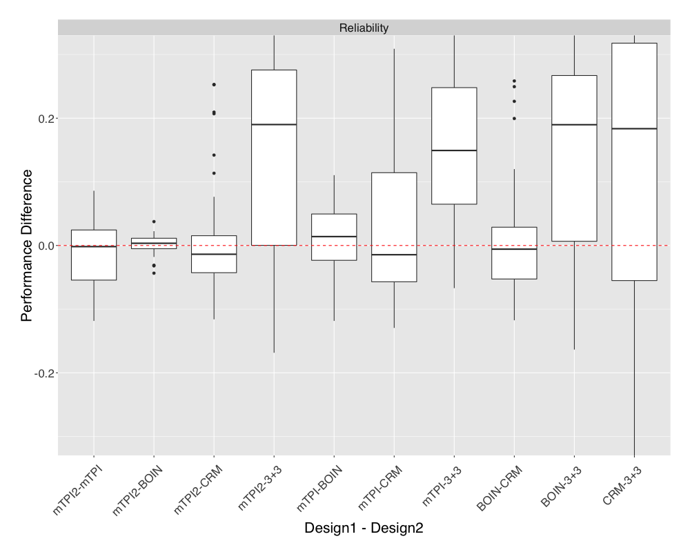
We implemented mTPI-2, mTPI, all three BOIN versions, CRM and 3+3 based on the 2,447 crowd-sourcing scenarios. For each scenario, 2,000 simulated trials were conducted on computer. We compared designs’ operating characters in terms of two simple metrics, safety and reliability (Ji and Wang, 2013). These two metrics capture the most important and fundamental properties of a dose-finding design: patient safety and ability to identify the true MTD. Safety is the average percentage of the patients treated at or below the true MTD across the simulated trials for a given scenario, and reliability is the percentage of simulated trials selecting the true MTD for a given scenario. In some literature, reliability is also called PCS, standing for the percentage of correct selection of the true MTD. Usually there is a tradeoff between the two metrics. That is, a design with better safety is usually associated with less reliability and vice versa. This is because in order to correctly identify the true MTD, a design must accurately infer doses both below and above the MTD, which means assigning some patients to doses above the MTD to learn their high toxicity probabilities. Doing that would lower the safety metric of the design.
 |
 |
Figure 3 presents the comparison results. For ease of exposition, we only show results from so that the interval boundaries among BOIN, mTPI, and mTPI-2 are the same. Results including and are shown in Appendix A. Overall, mTPI-2 is the safest design, putting more patients on average at doses at or below the MTD than the other four methods. BOIN is slightly worse than the mTPI-2 design on the safety measure, followed by mTPI, CRM, and 3+3. Except for 3+3, all the four model-based designs perform similarly in terms of reliability, i.e., the probability of identifying the true MTD, with mTPI-2 having slight advantage. The 3+3 design is the worst in the identification of the true MTD.
Results for set two.
Figure 4 shows the same comparison of the five designs based on the 42 scenarios (Appendix B) in Ji and Wang (2013), with 14 scenarios for each of the three values, 0.1, 0.2, and 0.3. As can be seen, mTPI-2 is the safest design while CRM edges mTPI in reliability, followed closely by mTPI-2 and BOIN. Again, the 3+3 design is the worst in both safety and reliability.
 |
 |
Results for set three.
The purpose of having set three is to examine the performance of all the designs when scenarios are systematically generated from the stochastic model in Paoletti et al. (2004). For illustration purpose, we assumed , cohort size 1, and six doses per scenario. We simulated 2,000 trials per scenario and presented the pair-wise comparison of the mTPI-2, mTPI, CRM, and BOIN designs using two criteria : 1) PCS: the percentage of trials of correct selection of the true MTD (this is the same as reliability); 2) Accuracy index for patient allocation (Cheung, 2011): a value that measures how accurate patients are allocated to the MTD and equals 1 when all the patients are allocated at the true MTD. Results are presented in Figure 5. Overall, mTPI-2, CRM and BOIN perform very similarly. As shown in previous work (Horton et al., 2016) the CRM and BOIN designs perform well in these scenarios. The mTPI design is slightly worse than the other three designs due to its stickiness (Guo et al., 2017) as a result of Occam’s razor. The mTPI-2 design presents comparable performance.
 |
| Scatter plots of PCS |
 |
| Scatter plots of Accuracy Index for subjects allocation |
4 Evaluation of Decision Tables
As in Section 3 and the vast literature, the gold standard of comparing different dose-finding methods is the operating characteristics (OC) from running a large number of simulated clinical trials on computer, with randomly generated data based on prespecified scenarios that determine the true toxicity probabilities of the candidate doses. While this provides a large-sample (of trials) and population-level assessment on the performance of the methods, it does not evaluate designs in terms of per-trial and per-patient behavior. For example, results in Figures 3 compare the distributions of the safety and reliability values for each design when tested on millions of simulated trials. But for an individual investigator, the trial at hand is of the most consideration. Practically, these OC results are not well understood by the clinical society and are often perceived as a “black-box” operation. Also, due to lack of user-friendly tools, it is challenging to generate the OC results for multiple dose-finding designs in practice. One of the key features for the 3+3 design is its transparent nature as all the decision rules can be prespecified and assessed without the need of running simulation. This same feature is also enjoyed by interval-based designs. For this reason, we propose to simply evaluate different designs based on the decision tables that consist of the dose-assignment decisions of each design. This evaluation can be added to the classical OC tables. For example, Figure 6 provides a decision table of mTPI-2 based on and for up to 15 patients. Such a table allows investigators to examine all the possible decisions before the trial starts. We denote such a table as which consists of decisions of mTPI-2 for values of , , and up to patients and possible DLT outcomes. Here takes three values {D, S, E} to denote the three up-and-down dose-assignment decisions. All the interval-based designs, mTPI-2, mTPI, and BOIN can provide such a table prior to the trial starts, and one common feature across the three designs is that the table entry is fixed given and for fixed and . For example, when 1 out of 3 patients experiences DLT, the table in Figure 6 shows the decision S, which is to stay at the current dose. This decision is applied to any dose level and any trial with .
For CRM, the table does not depend on since CRM does not require input of these two values. More importantly, each entry is not fixed but a random variable that follows a probability distribution depending on the probability model in the CRM design and the true toxicity probabilities of the doses. For example, consider a trial targeting . If 1 out of 3 patients experiences DLT, CRM will have a large probability (not equal to 1) to S, stay, but also small probabilities to E or D, depending on the patients data on other doses. Unfortunately, the probability distribution of cannot be derived analytically as it requires integration of all the possible outcomes of the trials that would have 1 DLT out of 3 patients at any dose. Instead, an investigator can obtain a numerical approximation of the random decision table under CRM based on the same computer simulated trials for generating the operating characteristics, and examine the approximated decision table carefully before proceeding. To see this, we provide an example next. Suppose we want to design a dose-finding trial with six doses, cohort size 3, and MTD target . We apply CRM to the 14 scenarios in Ji and Wang (2014) with (Appendix B) and sample size 51. We simulate 10,000 trials per scenario on computer using the R package dfCRM (https://cran.r-project.org/web/packages/dfcrm/index.html). We then tabulate the frequencies of the decisions D, S, or E that CRM takes whenever out of patients experience DLT in the simulated trials. These frequencies are the empirical distribution of the random decision under CRM since they are integrated over the data from a large number of simulated trials under various scenarios. In other words, this can be considered as a Monte Carlo approximation of the true distribution of Note that the actual CRM decisions specify the exact dose level for the next cohort of patients, but these decisions can be easily converted to D, S, or E based on the decided dose level and the current dose level. Therefore only takes D, S, or E, and we obtain three proportions for each and , where The results are summarized as a decision table in Figure 7 for up to 15 patients. We removed results for more than 15 patients for ease of exposition. This table allows investigators to examine the specific CRM method (in our case, the CRM is the one from the dfCRM R package) and its performance under the specific trial setting (, cohort size 3, and sample size 51) using a specific set of scenarios. For example, it can be seen from the table that more than half of the times the CRM design would stay when 1 out of 3 patients experienced DLT at a given dose (the yellow segment being longer than the blue segment in the bar for 1 DLT and 3 patients). When 2 out of 3 patients experienced DLT, about half of the times CRM would de-escalate but the other half of the times it would stay. These percentages various decisions are important for investigators and review boards to assess the performance of CRM and any designs being considered. And importantly, they are more intuitive and transparent than the OC results.
As a comparison, we also obtain the fixed decision tables (not shown) for a sample size of patients for the mTPI-2 and BOIN designs given value and a pair of values, denoted as and . Since these tables not only depend on values, but also , we vary both ’s from 0.005 to 0.05. For CRM, for each value we obtain three proportions which represent the proportions of the three decisions. As a summary, we compute the mean decision score defined as for each and value, where values , , and are assigned to decision , , and , respectively. Therefore, a higher value is associated with a more conservative decision. Figure 8 shows the sum of the differences (Design1 - Design2) of for mTPI-2 and BOIN and for CRM between any two designs for each of three values, and . For example, the top left panel presents the differences for all the values. A positive or negative value in the plot implies that Design1 is more likely to de-escalate or escalate, respectively. Overall mTPI-2 appear to have more de-escalation decisions than the other two designs in most cases, and the two interval-based designs do not differ much in general. The differences of the two designs get larger for larger values. CRM is in general more aggressive in its decisions than mTPI-2 and BOIN. However, when is large and is small, the equivalence interval becomes more skewed towards right, which means mTPI-2 and BOIN will be less likely to de-escalate and more likely to escalate. Therefore, we see the decisions of mTPI-2 and BOIN are more aggressive than CRM in these values (upper left corner of the heatmaps in Figure 8).


 |
 |
 |
 |
 |
 |
 |
 |
 |
5 Discussion
We show using crowd-sourcing results that mTPI, mTPI-2, and BOIN designs are superior than 3+3 and compare well with other non-interval designs, such as CRM. Due to the simplicity in the implementation of the interval designs, we recommend the use of these designs for practical trials. In particular, mTPI-2 seems to stand out with its rigorous theoretical development, superior numeric performance, simplicity in the implementation, and adherence to the ethical principle in its dose escalation decisions.
The interval designs can be categorized as the iDesigns, including TPI, mTPI, and mTPI-2, and IB-Designs including CCD and BOIN. They differ in the statistical inference and underlying decision strategies. Interestingly, they are very similar in implementation which produces a fixed decision table and is attractive to practitioners due to its simplicity and transparency. The use of deterministic decisions allow their decision tables to be calculated and examined prior to the trial onset, allowing investigators to see the behavior of the designs given various patient outcomes in terms of number of DLTs out of patients treated at a dose. The mTPI-2 design appears to have the best overall performance in our comparison using the the 42 scenarios in Ji and Wang (2013). The performance of mTPI-2 is similar to BOIN on overall reliability or PCS using the randomly generated scenarios. However, the decision tables give clear contrast that mTPI-2 is a safer design.
We also show that running a large number of computer simulated clinical trials and comparing operating characteristics of the designs is not sufficient to fully assess dose-finding designs in practice. We recommend to examine the decision tables, even for methods like CRM when its decision tables are not deterministic. Since a large number of simulated trials are usually conducted on computer as a standard practice, one can quickly generate the empirical distributions of the CRM decisions as in Figure 7 to assess the performance of CRM for a given pair of values. Decision tables and operating characteristics tables will jointly allow investigators to evaluate the population-level (across many simulated trials) and individual-level (across patients) behavior of a design. Therefore, both of them should be reviewed when these designs are considered for a practical trial.
Acknowledgement
This is a collaborative research with Dr. Sue-Jane Wang from US FDA. She provided numerous insightful critiques, did some technical investigations and gave constructive inputs throughout the research. We sincerely thank her for her professional expertise and scientific collaboration.
References
- Akaike (1974) Akaike, H. (1974). A new look at the statistical model identification. IEEE transactions on automatic control, 19(6):716–723.
- Babb et al. (1998) Babb, J., Rogatko, A., and Zacks, S. (1998). Cancer phase I clinical trials: efficient dose escalation with overdose control. Statistics in medicine, 17(10):1103–1120.
- Berger (2013) Berger, J. O. (2013). Statistical decision theory and Bayesian analysis. Springer Science & Business Media.
- Blanchard and Longmate (2011) Blanchard, M. S. and Longmate, J. A. (2011). Toxicity equivalence range design (teqr): a practical phase i design. Contemporary clinical trials, 32(1):114–121.
- Cheung (2011) Cheung, Y. K. (2011). Dose finding by the continual reassessment method. CRC Press.
- Cheung and Chappell (2002) Cheung, Y. K. and Chappell, R. A. (2002). A simple technique to evaluate model sensitivity in the continual reassessment method. Biometrics, 58(3):671–674.
- Clertant and O’Quigley (2017) Clertant, M. and O’Quigley, J. (2017). Semiparametric dose finding methods. Journal of the Royal Statistical Society, Series B, 79(3):10.1111/rssb.12229.
- Gezmu and Flournoy (2006) Gezmu, M. and Flournoy, N. (2006). Group up-and-down designs for dose-finding. Journal of statistical planning and inference, 136(6):1749–1764.
- Goodman et al. (1995) Goodman, S. N., Zahurak, M. L., and Piantadosi, S. (1995). Some practical improvements in the continual reassessment method for phase I studies. Statistics in medicine, 14(11):1149–1161.
- Guo et al. (2017) Guo, W., Wang, S.-J., Yang, S., Lin, S., and Ji, Y. (2017). A Bayesian Interval Dose-Finding Design Addressing Ockham’s Razor: mTPI-2. Contemprary Clinical Trials, in press.
- Ivanova et al. (2007) Ivanova, A., Flournoy, N., and Chung, Y. (2007). Cumulative cohort design for dose-finding. Journal of Statistical Planning and Inference, 137(7):2316–2327.
- Jefferys and Berger (1992) Jefferys, W. H. and Berger, J. O. (1992). Ockham’s razor and bayesian analysis. American Scientist, 80(1):64–72.
- Ji et al. (2007a) Ji, Y., Li, Y., and Bekele, B. N. (2007a). Dose-finding in phase I clinical trials based on toxicity probability intervals. Clinical Trials, 4(3):235–244.
- Ji et al. (2007b) Ji, Y., Li, Y., and Yin, G. (2007b). Bayesian dose finding in phase I clinical trials based on a new statistical framework. Statistica Sinica, pages 531–547.
- Ji et al. (2010) Ji, Y., Liu, P., Li, Y., and Bekele, B. N. (2010). A modified toxicity probability interval method for dose-finding trials. Clinical Trials, page 1740774510382799.
- Ji and Wang (2013) Ji, Y. and Wang, S.-J. (2013). Modified toxicity probability interval design: a safer and more reliable method than the 3+ 3 design for practical phase I trials. Journal of Clinical Oncology, 31(14):1785–1791.
- Liu and Yuan (2015) Liu, S. and Yuan, Y. (2015). Bayesian optimal interval designs for phase I clinical trials. Journal of the Royal Statistical Society: Series C (Applied Statistics), 64(3):507–523.
- O’Quigley et al. (1990) O’Quigley, J., Pepe, M., and Fisher, L. (1990). Continual reassessment method: a practical design for phase 1 clinical trials in cancer. Biometrics, pages 33–48.
- Paoletti et al. (2004) Paoletti, X., O’Quigley, J., and Maccario, J. (2004). Design efficiency in dose finding studies. Computational statistics & data analysis, 45(2):197–214.
- Schwarz et al. (1978) Schwarz, G. et al. (1978). Estimating the dimension of a model. The annals of statistics, 6(2):461–464.
- Storer (1989) Storer, B. E. (1989). Design and analysis of phase I clinical trials. Biometrics, pages 925–937.
- Stylianou and Flournoy (2002) Stylianou, M. and Flournoy, N. (2002). Dose finding using the biased coin Up-and-Down design and isotonic regression. Biometrics, 58(1):171–177.
- Yang et al. (2015) Yang, S., Wang, S.-J., and Ji, Y. (2015). An integrated dose-finding tool for phase I trials in oncology. Contemporary clinical trials, 45:426–434.
- Yuan et al. (2016) Yuan, Y., Hess, K. R., Hilsenbeck, S. G., and Gilbert, M. R. (2016). Bayesian optimal interval design: a simple and well-performing design for phase I oncology trials. American Association for Cancer Research, 22(17):4291–4301.
Appendix A
We present the pair-wise comparison of mTPI-2, mTPI, BOIN, CRM, and 3+3, with BOIN having three versions, The and versions are similar.
 |
 |
Appendix B
The 42 scenarios in Ji and Wang (2013) for and .
| Scenario # | Dose 1 | Dose 2 | Dose 3 | Dose 4 | Dose 5 | Dose 6 |
|---|---|---|---|---|---|---|
| = 0.1 | ||||||
| 1 | 0.04 | 0.05 | 0.06 | 0.07 | 0.08 | 0.09 |
| 2 | 0.15 | 0.2 | 0.25 | 0.3 | 0.35 | 0.4 |
| 3 | 0.01 | 0.1 | 0.2 | 0.25 | 0.3 | 0.35 |
| 4 | 0.01 | 0.02 | 0.03 | 0.04 | 0.1 | 0.25 |
| 5 | 0.05 | 0.4 | 0.5 | 0.6 | 0.65 | 0.7 |
| 6 | 0.01 | 0.03 | 0.05 | 0.4 | 0.5 | 0.6 |
| 7 | 0.01 | 0.02 | 0.03 | 0.04 | 0.05 | 0.4 |
| 8 | 0.09 | 0.11 | 0.13 | 0.15 | 0.17 | 0.19 |
| 9 | 0.05 | 0.07 | 0.09 | 0.11 | 0.13 | 0.15 |
| 10 | 0.01 | 0.03 | 0.05 | 0.07 | 0.09 | 0.11 |
| 11 | 0.02 | 0.04 | 0.08 | 0.12 | 0.17 | 0.25 |
| 12 | 0.02 | 0.04 | 0.07 | 0.1 | 0.15 | 0.2 |
| 13 | 0.1 | 0.15 | 0.2 | 0.25 | 0.3 | 0.35 |
| 14 | 0.01 | 0.03 | 0.05 | 0.06 | 0.08 | 0.1 |
| = 0.2 | ||||||
| 1 | 0.02 | 0.05 | 0.08 | 0.11 | 0.14 | 0.17 |
| 2 | 0.25 | 0.35 | 0.4 | 0.5 | 0.6 | 0.7 |
| 3 | 0.01 | 0.2 | 0.4 | 0.6 | 0.8 | 0.95 |
| 4 | 0.04 | 0.06 | 0.08 | 0.1 | 0.2 | 0.5 |
| 5 | 0.05 | 0.5 | 0.8 | 0.9 | 0.95 | 0.99 |
| 6 | 0.01 | 0.05 | 0.1 | 0.5 | 0.7 | 0.9 |
| 7 | 0.01 | 0.03 | 0.07 | 0.1 | 0.15 | 0.7 |
| 8 | 0.19 | 0.21 | 0.23 | 0.25 | 0.27 | 0.29 |
| 9 | 0.15 | 0.17 | 0.19 | 0.21 | 0.23 | 0.25 |
| 10 | 0.11 | 0.13 | 0.15 | 0.17 | 0.19 | 0.21 |
| 11 | 0.05 | 0.11 | 0.17 | 0.23 | 0.29 | 0.35 |
| 12 | 0.05 | 0.1 | 0.15 | 0.2 | 0.3 | 0.4 |
| 13 | 0.2 | 0.25 | 0.3 | 0.35 | 0.4 | 0.45 |
| 14 | 0.05 | 0.08 | 0.11 | 0.14 | 0.17 | 0.2 |
| = 0.3 | ||||||
| 1 | 0.02 | 0.05 | 0.1 | 0.15 | 0.2 | 0.25 |
| 2 | 0.35 | 0.45 | 0.5 | 0.6 | 0.7 | 0.8 |
| 3 | 0.01 | 0.3 | 0.55 | 0.65 | 0.8 | 0.95 |
| 4 | 0.04 | 0.06 | 0.08 | 0.1 | 0.3 | 0.6 |
| 5 | 0.05 | 0.6 | 0.8 | 0.9 | 0.95 | 0.99 |
| 6 | 0.01 | 0.05 | 0.1 | 0.6 | 0.7 | 0.9 |
| 7 | 0.01 | 0.03 | 0.07 | 0.1 | 0.15 | 0.75 |
| 8 | 0.29 | 0.31 | 0.33 | 0.35 | 0.37 | 0.39 |
| 9 | 0.25 | 0.27 | 0.29 | 0.31 | 0.33 | 0.35 |
| 10 | 0.21 | 0.23 | 0.25 | 0.27 | 0.29 | 0.31 |
| 11 | 0.05 | 0.2 | 0.27 | 0.33 | 0.39 | 0.45 |
| 12 | 0.05 | 0.1 | 0.2 | 0.3 | 0.4 | 0.4 |
| 13 | 0.3 | 0.35 | 0.4 | 0.45 | 0.5 | 0.55 |
| 14 | 0.15 | 0.18 | 0.21 | 0.24 | 0.27 | 0.3 |