Quasinormal modes of Einstein-Gauss-Bonnet-dilaton black holes
Abstract
We study quasinormal modes of static Einstein-Gauss-Bonnet-dilaton black holes. Both axial and polar perturbations are considered and studied from to . We emphasize the difference in the spectrum between the Schwarzschild solutions and dilatonic black holes. At large Gauss-Bonnet coupling constant a small secondary branch of black holes is present, when the dilaton coupling is sufficiently strong. The modes of the primary branch can differ from the Schwarzschild modes up to . The secondary branch is unstable and possesses long-lived modes. We address the possible effects of these modes on future observations of gravitational waves emitted during the ringdown phase of astrophysical black holes.
1 Introduction
The recent direct detections of gravitational waves by the LIGO/Virgo Collaboration [1, 2, 3] have fueled the interest in the study of black holes and neutron stars in astrophysical systems. The observational data are compatible with black hole mergers in general relativity (GR). The first observed event resulted in the formation of a black hole of , the second event resulted in a black hole, and the very recent third event resulted in a black hole. In the three cases, the estimated energy radiated in gravitational waves was about of the final black hole mass. However, although the detections from LIGO appear to be in good agreement with the predictions from GR, there is still plenty of room for alternative gravitational theories [4, 5, 6, 7, 8, 9, 10]. The study of black hole collisions in alternative theories of gravity, and, in particular, the study of the ringdown phase after the merger phase, can in principle be used to constrain those theories when compared with (future) observations.
In contrast to neutron stars, black holes are free from the extra complications introduced by high density states of matter. Gravitational waves radiated after the merger of black holes depend only on much simpler parameters, independently of how the gravitational waves have been triggered. The ringdown is determined by the three basic parameters of the final black hole, namely its mass, charge and angular momentum. In particular, the parameters of the final black hole produced after the merger can be inferred from the damped sinusoidal waves produced during the ringdown phase. The characteristic frequencies of these gravitational waves are given by the spectrum of quasinormal modes (QNM) of the black hole.
Although quasinormal modes contain the generic information on the source of the gravitational waves, the ringdown phase can differ in alternative theories of gravity from GR. The deviations in the QNM spectrum from GR predictions can be used to test alternative gravitational theories in the strong field regime. Additionally, a QNM analysis allows one to study the stability of black holes under linear mode perturbations.
From an observational perspective, the GR description of gravity may be questioned since it leads to an evolution of the Universe, that is currently dominated by the unknown constituents dark matter and dark energy. From the theoretical point of view an alternative theory of gravity is required in order to consistently formulate a quantum theory of the fundamental interactions. Here, one of the promising contenders for a new theoretical framework is string theory. In string theory, the Einstein-Hilbert term of GR will receive higher order corrections. For instance, the low-energy effective action as obtained from heterotic string theory will include a certain quadratic curvature term, the Gauss-Bonnet term, together with a coupling to a dilaton field [11, 12]. In particular, after compactification and truncation of extra gauge fields in heterotic string theory, an effective theory emerges containing both ingredients.
Thus inspired from string theory [13, 14, 15] Einstein-Gauss-Bonnet-dilaton (EGBd) theory is a gravitational theory which extends the Einstein-Hilbert action to include a dynamical scalar degree of freedom which is coupled to the Gauss-Bonnet invariant. In four dimensions, the Gauss-Bonnet invariant is topological, i.e., only a total derivative in the action, which would not modify the Einstein field equations by itself. But its non-minimal coupling to the dilaton field circumvents this. Moreover, despite the higher order curvature terms, the field equations of the theory remain second order in the derivatives. This ensures that no propagating ghost degree of freedom (in the sense of Ostrogradsky [16]) arises. Note, that the Gauss-Bonnet-dilaton term of the action also appears as an ingredient of a more general scalar-tensor theory (as the ‘Ringo’ term in the Fab-Four), which is directly related to a subsector of Horndeski gravity [17, 18].
Thus EGBd theory represents an interesting effective theory of gravity that can be tested by observations. It is viable on astrophysical scales [17]. In particular, it is in accordance with solar system observations and it allows for new effects and deviations from GR in strong fields. It features two coupling constants, the Gauss-Bonnet (GB) coupling constant and the dilaton coupling constant . There exist already some constraints imposed on the theory from astronomical observations [19], which have been derived for the (heterotic string theory) value . Measurement of the Shapiro time delay from the Cassini mission imposes a mild upper limit on the GB coupling constant, [20]. A stronger constraint is obtained from the observation of the low-mass X-ray binary A0620-00, based on the orbital decay rate in a black hole [21]. This observation constrains the maximum value of the possible dilaton charge, and hence the coupling constant [22].
Black hole solutions of EGBd theory could not be found in analytical form. Thus, static EGBd black hole solutions were first studied perturbatively [13, 14] and then numerically [15, 23]. Recently, the numerical solution has been analytically approximated in [24] using a continued fraction expansion. These EGBd black holes carry nontrivial dilaton fields outside their horizon. The presence of the Gauss-Bonnet-dilaton terms in the generalized Einstein equations lead to an “effective” energy-momentum tensor, allowing for negative “effective” energy densities and thus an evasion of the classical “no-scalar-hair” theorem [15]. Furthermore, the early studies [15] of static EGBd black holes showed already that the domain of existence of these solutions is bounded by a maximum value of the GB coupling parameter . Depending on the value of the dilaton coupling , close to the maximum of a short secondary branch of black hole solutions can arise [23, 25].
Rotating EGBd black holes were studied in the slow rotation approximation in [26, 27, 28, 29], and in the fast rotating case in [30, 31, 32]. Analogously to the static case, the domain of existence is bounded. The effect of rotation is to cause an effective reduction in the range of the coupling constant, where rotating black hole solutions exist. Interestingly, the rapidly rotating EGBd black holes can slightly exceed the Kerr bound for the angular momentum, and their quadrupole moments and moments of inertia can deviate significantly from the respective Kerr values. However, their shadows are very close to the shadows of Kerr black holes [33], and an analogous observation holds for their X-ray reflection spectrum [34].
Stability of the static EGBd black holes was studied in [35, 36], showing stability with respect to radial fluctuations for black holes on the primary branch, but revealing instability on the short secondary branch. First studies of axial and polar gravitational perturbations were done in [26, 37], indicating linear mode stability of the black holes on the primary branch. A similar conclusion was reached in [38], where the polar sector was analyzed in the high-frequency, geometric optics approximation.
In this paper we continue the analysis of the quasinormal modes of static EGBd black holes performed in [37]. We present results for quasinormal modes from to , in the axial and polar perturbations. We focus on perturbations on the full numerical background. This also allows us to conduct a closer inspection of the quasinormal modes close to the maximal value of the GB coupling constant, where the effect of the dilaton field is strong. The quasinormal mode analysis reveals a complicated structure in the spectrum close to this value, which might have observational implications. Our results from the analysis of quasinormal modes support both the linear mode stability of the static EGBd black holes on the primary branch, as well as the instability of the solutions belonging to the short secondary branches, which can be present for large values of the coupling (depending on the value of the dilaton coupling ) [25, 36]. Finally, using results from the recent observation of gravitational waves GW151226 [2], we discuss how EGBd theory could show its effects on the ringdown frequencies in black hole mergers. Moreover we address the bounds of the coupling constants.
2 Static black holes in Einstein-Gauss-Bonnet-dilaton theory
2.1 Theoretical framework
In four dimensions, the Einstein-Gauss-Bonnet-dilaton action is given by [15]
| (1) |
in natural units , where the first term in the action is the standard Einstein-Hilbert term, followed by the kinetic term for the dilaton field . is the Gauss-Bonnet term
| (2) |
which is coupled to the dilaton via the GB coupling constant and the dilaton coupling constant .
The field equations for the metric in this theory are
| (3) |
where is the usual Einstein tensor, and the gravitational terms on the right hand side arise due to the coupling to the dilaton field, where
| (4) | |||
| (5) |
does not contribute, since this tensor vanishes in four dimensions. The dilaton field equation is obtained from the variation of the action with respect to
| (6) |
From the field equations (3) and (6) it is clear that they are at most second order in the derivatives.
An interesting limit of the theory is obtained when the dilaton coupling is linear. This case can be obtained by modifying the Gauss-Bonnet term in the previous action Eq.(1): . The linear dilaton coupling can be understood as the first nontrivial term of the small limit in the exponential coupling. Note that then becomes trivial since it can be absorbed by redefining without loss of generality.
To describe static, spherically symmetric black holes we consider the following ansatz for the metric
| (7) |
The metric functions and , together with the dilaton field are functions of the radial coordinate , and can be obtained by inserting the ansatz into the equations (3)-(6) and then solving the resulting system of coupled ordinary differential equations numerically, subject to appropriate boundary conditions.
The black hole solutions are characterized by the presence of an event horizon at , where
with a constant coefficient , and
where the constant is given in terms of the constant that satisfies
| (8) |
is the dilaton value at the horizon. This is a quadratic equation for , which should have real solutions, so that the dilaton field is regular and possesses a real valued expansion near the horizon. Consequently the radicand of the solutions for should not become negative, and this requires that regular black hole solutions satisfy the inequality
| (9) |
It is this inequality, which leads to the theoretical bound on the GB coupling or the product , when is varied [15].
Asymptotically the solutions approach the Schwarzschild spacetime, which means , , and . Thus the mass of the black holes and the dilaton charge can be read off asymptotically. is another expansion constant.
2.2 Static black holes
Let us now briefly summarize the relevant properties of the static EGBd black hole solutions. As noted in [15], these black hole solutions possess a nontrivial dilaton field. Since the dilaton charge does not represent an additional conserved charge of the system, the black holes possess only secondary hair [39]. Thus, for a given value of the GB coupling constant (and the dilaton coupling constant ), the static black holes form a one parameter family of solutions, labeled for instance by the black hole mass or by the black hole horizon area .
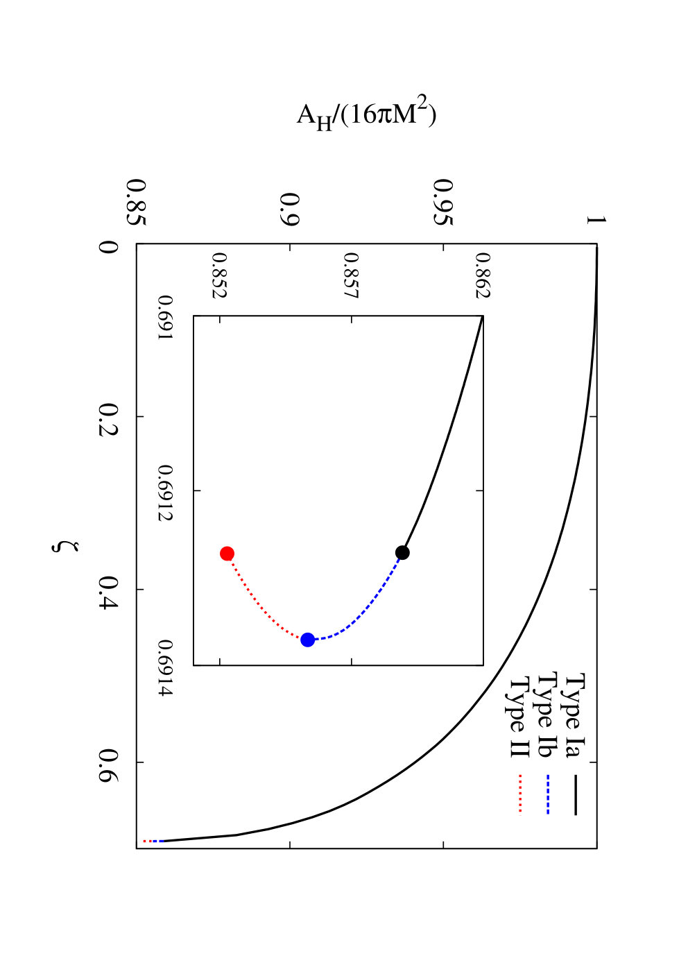
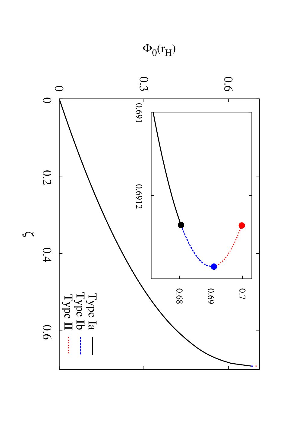
Another interesting property of these black holes noted in [15] is that their domain of existence is bounded. To illustrate this we present in Fig.1 the domain of existence of the static black holes for the value of the dilaton coupling constant , the value most explored in the literature so far. In Fig.1(a) we exhibit the scaled area of the black hole horizon of static EGBd black holes as a function of the scaled GB coupling constant . (The normalization is chosen such that the Schwarzschild black holes at possess the value .) Fig.1(b) represents a similar plot for the value of the dilaton field at the horizon .

Starting from the Schwarzschild value, the area decreases as the scaled GB constant rises together with the value of the dilaton field at the horizon. However, for , the branch of solutions extends only up to a maximal value of the scaled GB coupling, (marked by the blue dot in Fig.1). In fact, no regular black hole solutions exist for . Instead there arises a secondary branch of black hole solutions, residing between and [15, 26].
The main or primary branch of EGBd solutions thus extends from the Schwarzschild black holes () to the maximal value of the GB coupling . The black holes on this branch are named type I black holes, and fall into two subtypes, which join at (black dot). The type Ia black holes (black line) represent unique solutions, while the type Ib black holes (blue line) are no longer unique, since for a given value of in the range there are always two distinct static black hole solutions with the same mass. However, the two solutions can be distinguished by their differing horizon properties and dilaton charge. The type I black holes are regular on and outside their horizon for every value of , where they exist.
The primary branch ends at (blue dot), where it merges with the secondary type II branch. Note that precisely at the merger point uniqueness is recovered and only a single black hole solution is found. The secondary branch of type II black holes extends backwards from to (red dot). At a critical configuration is encountered, where the horizon expansion saturates the reality condition Eq.(9) for the dilaton field. However, this critical configuration is no longer regular [23, 25]. The figures illustrate, that type II solutions possess a smaller horizon area and a larger value of dilaton field at the horizon than type I solutions. In general, the black hole horizon area decreases when the dilaton field value gets larger. That is, black holes with a larger horizon have a weaker dilaton field at the horizon.
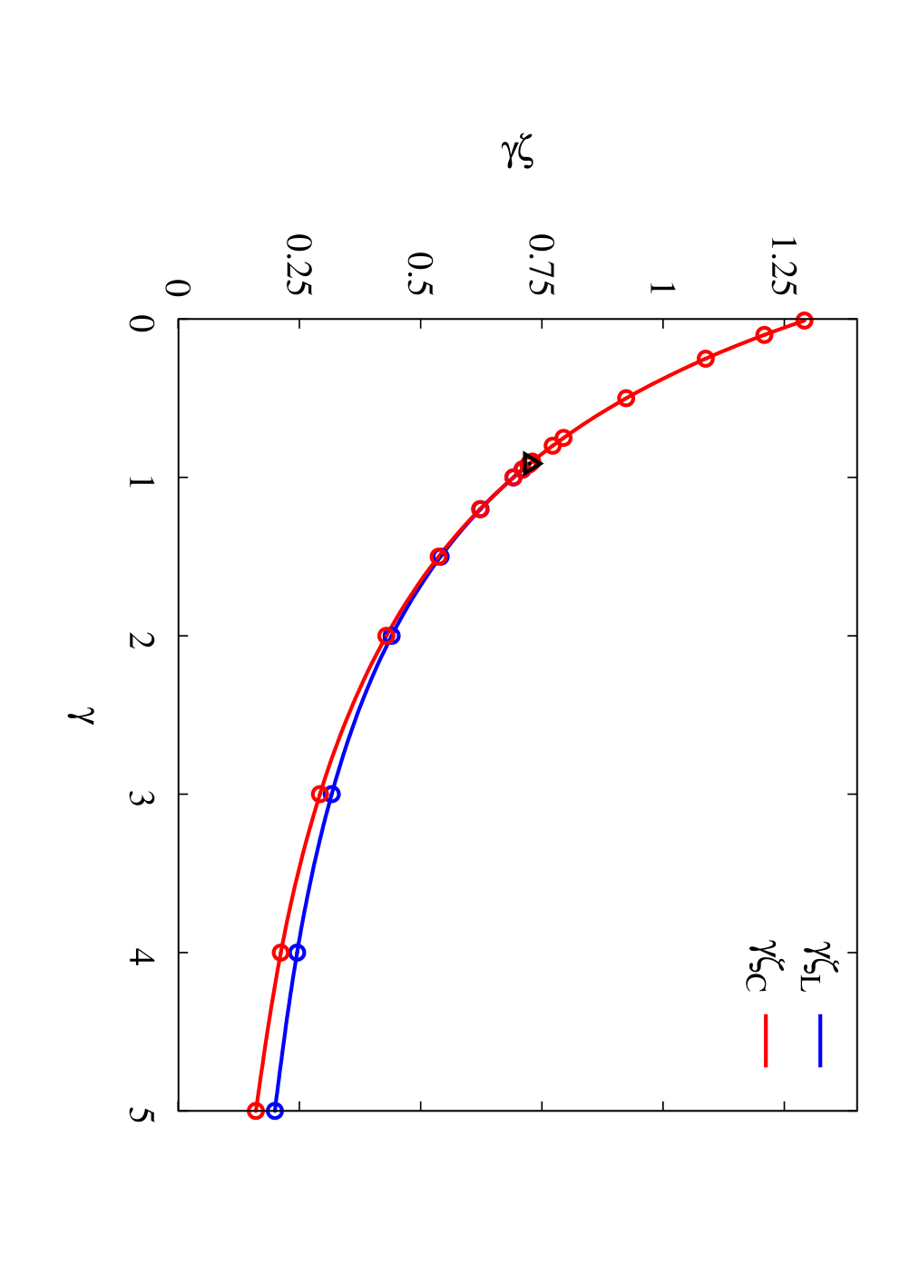
This branch structure is not only found for , but it occurs as well for other values of the dilaton coupling constant [25, 33]. In Fig.2 we illustrate the dependence of the maximal value and the critical value on the dilaton coupling constant . Starting from , an increase of leads to a rapid decrease of both and , and thus a rapid decrease of the domain of existence of static EGBd black hole solutions. At the same time, as the primary branch decreases in length, the length of the secondary branch increases, as seen in Fig.2(a). On the other hand, when starting from and decreasing , and rise rapidly, while their difference diminishes fast. The latter is illustrated in Fig.2(b), which reveals that the secondary branch ceases to exist close to .

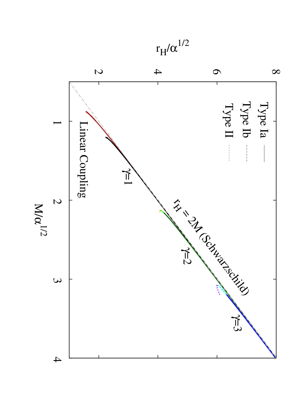
In Fig.3(a) we exhibit the scaled black hole horizon area versus for and and the linear coupling case. Again, the type Ia, Ib and II branches are presented by different colors and line styles. In particular, it can be seen that the size of the domain of existence decreases with (since decreases as increases), while the relative size of the second branch increases with . Note that in the linear coupling case, there are no type II black holes, but the domain of existence is also bounded.
The fact that the domain of existence is bounded by means that there is a minimum size for the static black holes of EGBd theory, when particular values of and are selected. To show this we present in Fig.3(b) the scaled horizon radius versus the scaled mass for three values of and the linear coupling case. For a given , the configuration residing at has the minimal value of the mass, while the configuration at has again a higher mass. Note, that for the scaled horizon radius is increasing again on the secondary branch (for fixed ).
Although in this paper we will focus on these static configurations, the effect of rotation on the properties of the EGBd black holes has been studied both perturbatively [26, 27, 28, 29], and nonperturbatively [30, 31, 32]. In the rotating case the domain of existence is also bounded, and the boundaries are given by the Kerr black holes, by the static EGBd black holes, by the set of critical EGBd black holes and by the set of extremal EGBd black holes. With increasing scaled angular momentum the associated value of decreases, until the Kerr bound is reached. Beyond the Kerr bound, there is also a finite lower limit for , which merges with at the configuration, where the maximum value of is attained.
3 Perturbations of Einstein-Gauss-Bonnet-dilaton black holes
3.1 Setup
In this section we lay out the quasinormal mode formalism, and the method used to study the QNM spectrum.
Since there are two dynamical fields in the theory, we perturb the metric and dilaton field separately as
| (10) | |||
| (11) |
where is the perturbation parameter. The zeroth order of each of the configurations is a static, spherically symmetric background described in the previous section, while the perturbations are time-dependent and not spherically symmetric.
Assuming that the nontrivial perturbation functions can be decomposed into the product of radial, temporal and angular parts, we use bases of spherical harmonic tensors to decouple the perturbations into two classes: the axial and polar perturbations [40, 41, 42, 43]. Under a parity transformation, the spherical harmonics of the axial perturbations transform according to , while for polar perturbations they transform as . Since these two types of perturbations never mix, both channels can be studied separately as in the GR case.
For the axial part of the metric perturbations, using a Laplace transformation of the time dependence, the expression of the perturbed part of the metric is
| (12) |
in the order of in the rows and columns of the matrix, and we have defined the angular functions
| (13) |
Note that are functions of , which carry the integer angular numbers , and the complex frequency . The gauge freedom allows us to fix , which is known as the Regge-Wheeler gauge.
On the other hand, for polar perturbations in the metric, we have
| (14) |
where and . Recall that are the metric functions from Eq.(7). The functions depend on the radial coordinate , the angular numbers , , and the complex frequency . Similarly, we can choose the gauge-fixing .
Since the dilaton is a scalar field, it only experiences polar perturbations. Factorizing the perturbation function in a similar way we have
| (15) |
where depends on and , like the metric perturbation functions.
Note that in our convention, the temporal part of the perturbations is taken to be , where the wave frequency is a complex number, for . By using this ansatz for the axial and polar perturbations, we are able to decouple the differential equations into a set of ordinary differential equations in with an undetermined frequency .
Before proceeding to the analysis of the field equations, we should specify the proper behaviour of the waves close to the horizon and to infinity. In the tortoise coordinate , with , the waves should be purely ingoing at the horizon and purely outgoing at infinity. Approaching the horizon (), the radial part of the waves goes as and toward infinity () it goes as as . Considering the time dependence , the imaginary part corresponds to , where is the damping time. The waves will exponentially decay in time, when is negative.
3.2 Equations, boundary conditions and numerical method
The modified Einstein equations up to first order perturbations can be reduced to a minimal set of differential equations of the form:
| (16) |
where , . In the axial case and in the polar case . The matrix contains the coefficients of the equations, which are given by combinations of the functions of the static solution , the number (there is degeneracy with respect to ), and the frequency eigenvalue . Since these equations are lengthy, we refer the readers to previous papers, where the expressions have already been presented [26, 37, 44].
In principle, Eq.(16) can be packaged into a single time-independent second order differential equation, which takes the form of the Regge-Wheeler/Zerilli equation, , with the potential. In our case, is a combination of functions , which describes the axial perturbations. For the polar perturbations we have two coupled functions in , where is a combination of the functions . As an example, we show in Figure 4 the potential as a function of the radial coordinate , for different values of the parameter. Nonetheless, the first order differential equation system from Eq.(16) is sufficient for our purpose here.

The outgoing wave behavior of the perturbations at infinity imposes the following behavior on the axial perturbations:
| (17) | |||||
| (18) |
where the parameter satisfies
| (19) |
and and are determined by the asymptotic expansion of the static metric (see Sec.2).
In the case of polar perturbations, the functions behave like:
| (20) | |||||
| (21) | |||||
| (22) |
At the horizon, we require waves falling into the horizon. This means the axial functions have the following near-horizon expansion:
| (23) | |||||
| (24) |
The parameter satisfies:
| (25) |
where , and the parameters and are given by the expansion of the static solution near the horizon.
In the polar case, the behavior close to the horizon is:
| (26) | |||||
| (27) | |||||
| (28) |
The parameter satisfies:
| (29) |
where we define
| (30) | |||||
In order to generate the quasinormal modes, we use a numerical procedure that implements these differential equations together with boundary conditions that satisfy the previous expansions. The method essentially consists of the following steps:
First we generate numerically a static dilatonic black hole by solving the EGBd equations with the appropriate boundary conditions
[15].
The estimated relative error of the solutions is lower than for a mesh with more than points.
The next step is to choose a value of and a value of . By moving outside the horizon , we evaluate the previous boundary conditions at . Using a shooting method we generate a first solution of the perturbation equations from . Typically, . To calculate the coefficients of of Eq.(16), we use the numerical static solution with an interpolation. Similarly, we choose a large value of , and with a shooting method we generate a second solution from . Typically . Finally, we study the continuity between the first and the second solution at , which is typically around .
If the solution is continuous within a required precision,
then we take as the frequency of a quasinormal mode,
with number , of the black hole under consideration.
To find such solutions,
we implement a numerical procedure to explore the complex plane
for .
Typically we require to have a relative precision below .
In the following sections we present the numerical results, where we have varied the GB coupling constant , the dilaton coupling , the black hole mass , and the angular number .
4 Results and Discussion
4.1 Spectrum for fundamental modes of the type I black holes
In this section we will focus on the EGBd black holes on the primary branch, i.e., type I black holes, with a fixed dilaton coupling . Later (in Sec.4.3) we will discuss the effect of changing . We now begin by showing the complete set of results for the fundamental modes of the axial and polar perturbations.
In GR, gravitational waves are obtained starting from (quadrupole radiation), where typically and are expected to dominate any physically relevant signal. In addition, one can consider scalar modes and vector modes, by studying a field with spin propagating in the background of a Schwarzschild or Kerr black hole (see e.g. [45, 46]).
In EGBd theory, the situation changes somewhat, since with the dilaton field there is already a scalar field present in the background black hole solution, which can give rise to the emission of gravitational waves. Thus and modes are inherent to the theory, and their study is essential for a complete physical understanding. In particular, their study is necessary for an analysis of the linear mode stability. Considering only the metric and the dilaton field (and no further external fields), then all axial perturbations are gravitationally induced perturbations. In contrast, for the polar perturbations a new channel of gravitational radiation is obtained, with modes exciting both spacetime and scalar fluctuations, since the dilaton is dynamically coupled to the spacetime [22, 37].
4.1.1 monopole and dipole perturbations
In the following, we will present the results for the quasinormal modes in dimensionless quantities, by exhibiting the scaled frequency versus the scaled GB coupling constant .


When , we start from the corresponding modes for and for of external fields with spin in the background Schwarzschild metric. But as soon as assumes a finite value, and the black holes represent genuine EGBd black holes, the dilaton and metric perturbations are coupled. Thus the waves emitted in these channels carry a combination of dilaton and metric excitations.
In Fig.5 we present the frequencies of the fundamental and EGBd modes, where the real part is shown in Fig.5(a) and the imaginary part is shown in Fig.5(b).
For a fixed mass, the real part of the mode first decreases slightly from the Schwarzschild value with increasing , until around , shows a sharp decline, approaching zero at . However, rises again beyond . (Recall the maximal value .) In particular, black holes close to the limiting coupling constant have a nonvanishing real part of the frequency, , as we will show in Sec.4.2. The imaginary part of the frequency first increases slightly from the Schwarzschild value, then reaches a local maximum and next a local minimum, and then rises sharply, as it gets closer toward . It is important to note that for type I black holes, the value of remains always negative, which is important for their stability.
For the -dependence is very different. The real part of the frequency first decreases very slowly from the Schwarzschild value. For intermediate values of the coupling constant it slightly rises again, and then shows another small decrease toward . The same applies to the imaginary part of the frequency . Overall the mode is only very weakly dependent on . Thus the deviations from the mode in GR are rather small.
4.1.2 Axial fundamental modes for and


Let us now present the axial fundamental and modes. Axial perturbations describe pure spacetime perturbations. Therefore these perturbations are purely gravitational in nature with no excitation of the dilaton field. In principle such modes could be excited in a merger process.
Let us first recall the known GR values of the frequency for the fundamental modes. These are for , and for . To convert these values into Hz, one has to multiply by , where is the solar mass [47].
We present the frequencies of the axial fundamental EGBd modes in Fig.6 versus the scaled coupling constant . The left figures show the real part of the frequency, while the imaginary part is shown on the right.
Fig.6(a) shows that the real part increases slightly with the coupling constant for . This holds everywhere except in a small region close to , which we will explore in detail in Sec.4.2. The deviation from GR is very small, less than below , and only up to beyond. The imaginary part is shown in Fig.6(b). Again, the deviation from GR is very small for smaller values of the coupling. Around the mode becomes damped faster (the difference to GR rising up to ). Close to the dependence of becomes more complicated, and we will zoom into this region in Sec.4.2.
In Fig.6(c) and 6(d), we show the analogous figures for the axial fundamental mode as a function of . In Fig.6(c) we see that the real part increases quadratically with up to toward . The imaginary part, shown in Fig.6(d), however, hardly deviates from the GR value for intermediate values of , and it only decreases down to , when in the vicinity of . Overall, the variation of the axial fundamental mode with the coupling constant is quite small as compared to the mode.
4.1.3 Polar fundamental modes for and


The polar perturbations include the excitation of the dilaton field, and hence we find two channels for the gravitational wave emission. To classify these channels, we first recall that in GR the gravitational frequencies are the same in the axial and the polar case, i.e., there is isospectrality [48]. The frequencies are for and for . But in addition there are also the modes of a scalar field in the Schwarzschild background, for and for . Therefore, we refer to the modes arising in the limit from the gravitational modes as the gravitational-led modes, while we refer to the modes arising in the limit from scalar channel as the scalar-led modes.
In Fig.7 we present the polar fundamental modes versus the scaled coupling constant . In general, the gravitational modes in the polar channels show larger deviations from the known GR () values, as compared to their gravitational axial counterparts. In particular this means that the isospectrality of the axial and polar spectrum present for Schwarzschild black holes is broken in EGBd theory.
In Fig.7(a) we show the real part of the gravitational-led polar fundamental mode. As the GB coupling constant increases, the frequency decreases. This is opposite to what happens for the axial mode shown in Fig.6(a). The reduction of is, however, relatively small (below ).
The imaginary part of the gravitational-led polar mode is shown in Fig.7(b) as a function of . As compared to GR, this mode tends to be more rapidly damped in EGBd black holes for configurations below (around a ). However, for larger values of the coupling, the imaginary part decreases rapidly, resulting in more slowly damped modes than in the GR case. The structure close to is more complicated, and we will comment more on it in Sec.4.2.
Let us now address the scalar-led modes. In Fig.7(c) we present the real part of the fundamental scalar-led mode as a function of , and in Fig.7(d) we present the corresponding imaginary part.
Fig.7(c) shows that for small values of the coupling constant, the real part of the frequency is slightly smaller for EGBd black holes than for Schwarzschild black holes. However, the frequency grows with the coupling from onward. Around the limiting coupling the frequency is about larger than in the GR case.
The imaginary part decreases with the coupling, as seen in Fig.7(d). Again, although for intermediate values of the coupling the difference with respect to GR is not very large (up to around ), close to the limiting coupling the damping time can be much smaller than the GR case, as we will show in Sec.4.2.


Similar figures for the modes are shown in Fig.8 for the gravitational-led and the scalar-led modes. The general behavior is similar to the modes. However, it is interesting to note that when increasing the coupling to , the imaginary part of the gravitational-led mode increases significantly (Fig.8(b)), meaning that the EGBd mode is more rapidly damped than its GR counterpart.
4.2 Secondary branch instability
In this section we study the quasinormal modes of the EGBd black holes in the vicinity of the maximal GB coupling for dilaton coupling . At the secondary branch of static EGBd black hole solutions appears, as discussed in Sec.2.
In [36] an analysis of linear mode stability was performed for purely radial perturbations. This showed that the secondary branch is mode unstable. In contrast, the primary branch does not present any such sign of instability. This result is also in agreement with arguments from catastrophy theory [23].


In Fig.9 we exhibit a zoom into the region of the GB coupling close to . Employing the same color coding as in the figures of the solutions themselves, we highlight the behavior of the previously discussed mode in this region of the parameter space, which connects with the Schwarzschild mode in the limit . These modes with negative imaginary part are present for the type II as well as for the type I black holes. However, close to their imaginary part is much smaller than in the Schwarzschild case.
Interestingly, in addition to this branch of modes, which possesses a Schwarzschild limit, there is a distinct further branch of modes, which is present only for the solutions of the secondary branch. This branch of modes represents the unstable radial modes seen in [36]. These modes are purely imaginary, with the real part vanishing as seen in Fig.9(a). Fig.9(b) shows that imaginary part of these modes of the type II black holes resides in the positive half-plane. Thus these modes represent unstable modes. Considering the limit on the secondary branch, we note, that the imaginary part also vanishes there, and hence the mode disappears. Therefore these modes are not present on the primary branch of the type I black holes.


We exhibit in Fig.10 the fundamental modes close to . The real part of the axial fundamental mode, shown in Fig.10(a), demonstrates that type II black holes possess a lower frequency than type Ib black holes. The imaginary part displayed in Fig.10(b) is increasing with for the type Ib black holes, but decreasing again toward for the type II black holes.
The gravitational-led polar modes are exhibited in Fig.10(c) (real part ) and Fig.10(d) (imaginary part ). The frequency reaches a minimum at a particular type II configuration. Close to the frequency decreases continuously, but then rises sharply to at . The imaginary part shows a similar behavior, rising up to when approaching . Thus this mode of the type II black holes is much longer ( times) lived than the corresponding modes of the type I solutions. Such a behavior is compatible with the beginning of an instability [49].
The scalar-led polar mode, shown in Fig.10(e) and Fig.10(f), exhibits only little dependence on the primary branch close to , but a strong frequency increase of more than close to . The imaginary part features a cusp at where the imaginary part reaches a minimum, followed by a strong increase for the type II solutions, whose damping time can be longer than for type I black holes. This effect in the scalar-led mode is qualitatively similar but less dramatic than in the gravitational-led mode.
In summary, we have not found any signs of unstable modes in type I black holes, even close to . The imaginary part of the frequency of the modes always remains negative in type I solutions. However, we have confirmed previous results [36] showing that the modes of the black holes on the secondary branch, i.e., the type II black holes, are unstable. On the other hand, by studying the modes of the secondary branch we have seen that in the gravitational-led polar modes, the damping time of the type II black holes could be times longer than in case of type I black holes, if the instability in the channel could be avoided.
4.3 Effect of the dilaton coupling on the QNM spectrum


So far we have considered the QNM spectrum only for the case of dilaton coupling , i.e., the value motivated by string theory. In this section we will address the effects for the QNM spectrum obtained by varying the dilaton coupling . In particular, we first focus on the fundamental polar modes on the primary branch, and consider and .
In Fig.11 we present the real and imaginary parts of the gravitational-led modes (Fig.11(a) and 11(b), respectively) and the real and imaginary parts of the scalar-led modes (Fig.11(c) and 11(d), respectively). As is increased, the frequencies change faster with , but remain closer to the GR value, overall. This also holds for the damping times of the scalar-led modes, while the damping times of the gravitational-led modes reach similar minimal values for all values of considered. We have employed as the axis to demonstrate that the linear term dominates for a considerable range of values of the frequency, in particular, in the real part of the gravitational-led mode and the imaginary part of the scalar-led mode.

In Fig.12 we demonstrate the effect of the dilaton coupling on the instability of the black holes on the secondary branch. Since the real part of the corresponding unstable modes vanishes, we exhibit only the imaginary part versus the GB coupling. However, we here employ a normalized GB coupling , such that all three secondary branches start at the same point . We note that the configurations obtained for larger values of have a smaller for the same value of the mass and (within their domain of existence). However, for the larger values of the secondary branches extend further, and the imaginary parts increase the more toward with larger .
4.4 Astrophysical implications of the constraint on the Gauss-Bonnet coupling constant
Here we comment on what we can learn from these results for the application to observations. We will focus on the case with , although a change of the dilaton coupling does not affect the qualitative features we will describe.
The current upper limit for the GB coupling constant , as mentioned already, derives from observations X-ray binary A0620-00 and is given by cm. Making use of the theoretical limit shows that, if we assume a theory with cm and , the smallest possible mass of a static black hole in the universe would be .
On the other hand, the smallest stellar black hole candidate observed is in the X-ray transient GRO J0422+32. Originally, the central black hole of the binary system was thought to possess a mass of [50], but a more recent analysis of the data revealed a much smaller object with [51]. This has cast doubts on the actual nature of the object in GRO J0422+32, which may not be a black hole, but another type of compact configuration. Interestingly, if this object is excluded, the data reveals a mass-gap between stellar black holes and neutron stars, with the minimum mass of black holes being compatible with [51]. This mass-gap limit is for instance larger than the constraint imposed by A0620-00 on EGBd theory with cm and .
The second LIGO/Virgo observation, GW151226 [2] has detected gravitational waves from the coalescence of two stellar-mass black holes. The comparison of the signal with GR simulations established that the masses of the black holes were for the first black hole BH1, and for the second black hole BH2, which inspiraled and eventually merged. The resulting black hole BH3 had an estimated mass of . Since all these masses are larger than , these observations do not improve the constraint A0620-00 on EGBd theory with , assuming they can be described by static EGBd black holes.
Note that if one makes the same reasoning assuming instead rotating black holes in EGBd, the value of the constraint will be smaller since the effect of rotation is to decrease [32]. Observations appear to favour rotating black holes far from extremality [2], hence the assumption of static initial black holes can be taken as a sufficient approximation. Similarly, one can consider only smaller GB couplings to allow for a lower black hole mass, since the analysis of X-ray transients [51] suggests that the mass of stellar black holes can be equal or very close to the mass of large neutron stars ().
In Fig.13 we present the domain of existence of static black holes as a function of the mass in solar units, which is represented by the solid space in cyan. In blue we mark the limiting solutions with . In Fig.13(a) we show the domain for , and in Fig.13(b) for . We mark the upper bound of the constraint on the coupling constant of cm with an orange dashed line. On this line, in red, green and purple we mark BH1, BH2 and BH3 respectively. With a black asterisk we mark the mass of GRO J0422+32. Note that this object is outside of the region of regular EGBd solutions, which implies that if this object were in fact a black hole, the constraint on the space of parameters would be improved considerably (for , cm, and for , cm).


We can ask the question of how does the QNM spectrum look in the case of such a coupling constant. For instance, consider Fig.14, where we show the frequencies of the gravitational-led polar mode normalized to corresponding Schwarzschild values, plotted as a function of the mass. Assuming the effective theory has indeed cm, we show the deviation from GR of the real part (top) and imaginary part (bottom) as a function of the mass. The first thing to notice is that the final black hole with a mass around would present a QNM spectrum very similar to a GR black hole. The deviation in the ringdown frequency of the final BH3 configuration with with respect to the Schwarzschild black hole is , and in the imaginary part.
Note, that this value of supposes the most favorable scenario. If one considers smaller values of (hence allowing for an even smaller limit for the mass of black holes), the QNM spectrum in EGBd will be even closer to the GR description. Hence one can expect the ringdown phase of black holes far from to be very well described by GR, which makes the measurement of by gravitational wave observations challenging. Of course in such a scenario, it would be possible to detect the dilaton component in the gravitational wave, although its quasinormal modes will be very close to the ones of a test scalar field. We conclude that the GR values would represent a rather good approximation for the EGBd frequencies in the description of the GW151226 event.
In order to constrain the theory further, it would be much more favorable to obtain observations of the ringdown of configurations close to , since these would possess the largest deviations from GR in their spectrum. For instance, consider in Fig.14 solutions close to the maximal GB coupling (blue dot). Type I black holes then exhibit deviations from GR on the order of .
While the fundamental gravitational wave frequencies of type II black holes deviate even stronger from those of the Schwarzschild case, their radial instabilities should completely change the physical picture of the would-be ringdown phase.

5 Conclusions
We have continued the study of black hole quasinormal modes in EGBd theory started in [26, 37]. Such quasinormal modes are thought to describe the ringdown phase of an excited black hole, and can be detected by gravitational wave observatories such as LIGO/Virgo. The quasinormal modes contain the most direct and intrinsic information of a black hole, as from their detection the properties of the gravitational wave source can be inferred. Moreover, besides testing GR these observations can also constrain alternative theories of gravity such as EGBd theory.
Here we have further explored the linear mode stability of the static EGBd black holes. In particular, we have calculated the quasinormal modes from to in the full domain of existence of the EGBd black holes. Our results indicate the linear mode stability of the EGBd black holes on their primary branch (type I black holes). In agreement with previous results, we have found an instability in the spectrum of the black holes on the secondary branch (type II black holes), where the branch of unstable modes is purely imaginary. While the modes of these type II black holes could be very long-lived, this would require some mechanism to evade the unstable modes.
The EGBd black holes break the isospectrality known for black holes in GR. The black holes on the primary branch possess frequencies rather close to the respective GR frequencies, unless they reside in the vicinity of the maximal GB coupling . This value depends markedly on the value of the dilaton coupling . In fact, we have considered the effect of variations of on the QNM spectrum. The results show that the qualitative features of the case are also present for other values of the coupling, in particular, we have observed a milder effect of on the spectrum, and the continued presence of the instability on the second branch.

Our results suggest that constraining EGBd theory from the observation of the ringdown can be challenging. As an example, we have considered the black hole masses in the binary black hole coalescence GW151226, invoking the theoretical limit on (for different ). Considering the expected QNM frequencies have allowed us to see that even in the most favorable case, the final black hole of would be ringing at a frequency very close to Schwarzschild. This suggests that in order to measure or constrain the GB coupling constant from the detection of gravitational waves produced in the ringdown phase of black hole mergers, one would need black holes sufficiently close to the limiting GB coupling .
On the other hand, the observation of stellar black holes and the determination of their mass can be used to improve the constraint on the free parameters of EGBd theory, and . In Fig.15 we show the parameter space versus . The white line marks the constraint imposed by the X-ray binary A0620-00, and the blue dashed line the constraint imposed by the possible mass-gap. In red we mark the regions of the parameter space excluded by both limits, and in orange by one of them. The area in green represents values allowed by the observations. In addition we include the limit imposed by the possibility that GRO J0422+32 is a black hole with , marked with a pink dashed line. In this case, both constraints on EGBd theory with arbitrary are improved. The possible observation in the coming years of gravitational waves from small stellar mass black holes (if they exist) could be used to improve even more the current constraints of the parameter space of EGBd theory.
6 Acknowledgments
The authors thank Vitor Cardoso and Caio F. B. Macedo for helpful discussions. FSK thanks the University of Oldenburg and the University of Groningen for their kind hospitality. JLBS, FSK and JK gratefully acknowledge support by the DFG funded Research Training Group 1620 “Models of Gravity”. JLBS and JK gratefully acknowledge support from FP7, Marie Curie Actions, People, International Research Staff Exchange Scheme (IRSES-606096).
References
- [1] B. P. Abbott et al. Observation of gravitational waves from a binary black hole merger. Phys. Rev. Lett., 116:061102, Feb 2016.
- [2] B. P. Abbott et al. Gw151226: Observation of gravitational waves from a 22-solar-mass binary black hole coalescence. Phys. Rev. Lett., 116:241103, Jun 2016.
- [3] B. P. Abbott et al. Gw170104: Observation of a 50-solar-mass binary black hole coalescence at redshift 0.2. Phys. Rev. Lett., 118:221101, Jun 2017.
- [4] Mariafelicia De Laurentis, Oliver Porth, Luke Bovard, Bobomurat Ahmedov, and Ahmadjon Abdujabbarov. Constraining alternative theories of gravity using GW and GW. Phys. Rev., D94(12):124038, 2016.
- [5] Roman Konoplya and Alexander Zhidenko. Detection of gravitational waves from black holes: Is there a window for alternative theories? Phys. Lett., B756:350–353, 2016.
- [6] Vitor Cardoso, Edgardo Franzin, and Paolo Pani. Is the gravitational-wave ringdown a probe of the event horizon? Phys. Rev. Lett., 116:171101, Apr 2016.
- [7] Vitor Cardoso, Seth Hopper, Caio F. B. Macedo, Carlos Palenzuela, and Paolo Pani. Gravitational-wave signatures of exotic compact objects and of quantum corrections at the horizon scale. Phys. Rev., D94(8):084031, 2016.
- [8] Jahed Abedi, Hannah Dykaar, and Niayesh Afshordi. Echoes from the Abyss: Evidence for Planck-scale structure at black hole horizons. 2016.
- [9] Hiroyuki Nakano, Norichika Sago, Hideyuki Tagoshi, and Takahiro Tanaka. Black hole ringdown echoes and howls. 2017.
- [10] Dan B. Sibandze, Rituparno Goswami, Sunil D. Maharaj, and Peter K. S. Dunsby. Echoes from the black holes: Evidence of higher order corrections to General Relativity in strong gravity regime. 2017.
- [11] David J. Gross and John H. Sloan. The Quartic Effective Action for the Heterotic String. Nucl. Phys., B291:41–89, 1987.
- [12] R. R. Metsaev and Arkady A. Tseytlin. Order alpha-prime (Two Loop) Equivalence of the String Equations of Motion and the Sigma Model Weyl Invariance Conditions: Dependence on the Dilaton and the Antisymmetric Tensor. Nucl. Phys., B293:385–419, 1987.
- [13] S. Mignemi and N. R. Stewart. Charged black holes in effective string theory. Phys. Rev., D47:5259–5269, 1993.
- [14] S. Mignemi. Dyonic black holes in effective string theory. Phys. Rev., D51:934–937, 1995.
- [15] P. Kanti, N. E. Mavromatos, J. Rizos, K. Tamvakis, and E. Winstanley. Dilatonic black holes in higher curvature string gravity. Phys. Rev. D, 54:5049–5058, Oct 1996.
- [16] M. Ostrogradsky. Mem. Ac. St. Petersburg, VI 4:385, 1850.
- [17] Emanuele Berti et al. Testing General Relativity with Present and Future Astrophysical Observations. Class. Quant. Grav., 32:243001, 2015.
- [18] Andrea Maselli, Hector O. Silva, Masato Minamitsuji, and Emanuele Berti. Neutron stars in Horndeski gravity. Phys. Rev., D93(12):124056, 2016.
- [19] Jose Luis Blázquez-Salcedo et al. Black holes in Einstein-Gauss-Bonnet-dilaton theory. 2016.
- [20] B. Bertotti, L. Iess, and P. Tortora. A test of general relativity using radio links with the Cassini spacecraft. Nature, 425:374–376, 2003.
- [21] Andrew G. Cantrell, Charles D. Bailyn, Jerome A. Orosz, Jeffrey E. McClintock, Ronald A. Remillard, Cynthia S. Froning, Joseph Neilsen, Dawn M. Gelino, and Lijun Gou. The inclination of the soft x-ray transient a0620–00 and the mass of its black hole. The Astrophysical Journal, 710(2):1127, 2010.
- [22] Kent Yagi. A New constraint on scalar Gauss-Bonnet gravity and a possible explanation for the excess of the orbital decay rate in a low-mass X-ray binary. Phys. Rev., D86:081504, 2012.
- [23] Takashi Torii, Hiroki Yajima, and Kei-ichi Maeda. Dilatonic black holes with a gauss-bonnet term. Phys. Rev. D, 55:739–753, Jan 1997.
- [24] K. D. Kokkotas, R. A. Konoplya, and A. Zhidenko. An analytical approximation for the Einstein-dilaton-Gauss-Bonnet black hole metric. 2017.
- [25] Zong-Kuan Guo, Nobuyoshi Ohta, and Takashi Torii. Black Holes in the Dilatonic Einstein-Gauss-Bonnet Theory in Various Dimensions. I. Asymptotically Flat Black Holes. Prog. Theor. Phys., 120:581–607, 2008.
- [26] Paolo Pani and Vitor Cardoso. Are black holes in alternative theories serious astrophysical candidates? the case for einstein-dilaton-gauss-bonnet black holes. Phys. Rev. D, 79:084031, Apr 2009.
- [27] Paolo Pani, Caio F. B. Macedo, Luis C. B. Crispino, and Vitor Cardoso. Slowly rotating black holes in alternative theories of gravity. Phys. Rev., D84:087501, 2011.
- [28] Dimitry Ayzenberg and Nicolas Yunes. Slowly-Rotating Black Holes in Einstein-Dilaton-Gauss-Bonnet Gravity: Quadratic Order in Spin Solutions. Phys. Rev., D90:044066, 2014. [Erratum: Phys. Rev.D91,no.6,069905(2015)].
- [29] Andrea Maselli, Paolo Pani, Leonardo Gualtieri, and Valeria Ferrari. Rotating black holes in Einstein-Dilaton-Gauss-Bonnet gravity with finite coupling. Phys. Rev., D92(8):083014, 2015.
- [30] Burkhard Kleihaus, Jutta Kunz, and Eugen Radu. Rotating black holes in dilatonic einstein-gauss-bonnet theory. Phys. Rev. Lett., 106:151104, Apr 2011.
- [31] Burkhard Kleihaus, Jutta Kunz, and Sindy Mojica. Quadrupole Moments of Rapidly Rotating Compact Objects in Dilatonic Einstein-Gauss-Bonnet Theory. Phys. Rev., D90(6):061501, 2014.
- [32] Burkhard Kleihaus, Jutta Kunz, Sindy Mojica, and Eugen Radu. Spinning black holes in Einstein–Gauss-Bonnet-dilaton theory: Nonperturbative solutions. Phys. Rev., D93(4):044047, 2016.
- [33] Pedro V. P. Cunha, Carlos A. R. Herdeiro, Burkhard Kleihaus, Jutta Kunz, and Eugen Radu. Shadows of Einstein–dilaton–Gauss–Bonnet black holes. Phys. Lett., B768:373–379, 2017.
- [34] Hao Zhang, Menglei Zhou, Cosimo Bambi, Burkhard Kleihaus, Jutta Kunz, and Eugen Radu. Testing Einstein-dilaton-Gauss-Bonnet gravity from the reflection spectrum of accreting black holes. Phys. Rev., D95:104043, 2017.
- [35] P. Kanti, N. E. Mavromatos, J. Rizos, K. Tamvakis, and E. Winstanley. Dilatonic black holes in higher curvature string gravity. 2: Linear stability. Phys. Rev., D57:6255–6264, 1998.
- [36] Takashi Torii and Kei-ichi Maeda. Stability of a dilatonic black hole with a gauss-bonnet term. Phys. Rev. D, 58:084004, Aug 1998.
- [37] Jose Luis Blázquez-Salcedo, Caio F. B. Macedo, Vitor Cardoso, Valeria Ferrari, Leonardo Gualtieri, Fech Scen Khoo, Jutta Kunz, and Paolo Pani. Perturbed black holes in Einstein-dilaton-Gauss-Bonnet gravity: Stability, ringdown, and gravitational-wave emission. Phys. Rev., D94(10):104024, 2016.
- [38] Dimitry Ayzenberg, Kent Yagi, and Nicolas Yunes. Linear Stability Analysis of Dynamical Quadratic Gravity. Phys. Rev., D89(4):044023, 2014.
- [39] K. Hajian and M. M. Sheikh-Jabbari. Redundant and Physical Black Hole Parameters: Is there an independent physical dilaton charge? Phys. Lett., B768:228–234, 2017.
- [40] Kip S. Thorne. Multipole expansions of gravitational radiation. Rev. Mod. Phys., 52:299–339, Apr 1980.
- [41] T. Regge and J. A. Wheeler. Stability of a Schwarzschild Singularity. Phys. Rev., 108:1063–1069, November 1957.
- [42] Frank J. Zerilli. Effective potential for even-parity regge-wheeler gravitational perturbation equations. Phys. Rev. Lett., 24:737–738, Mar 1970.
- [43] L. Fernandez-Jambrina and L. M Gonzalez-Romero, editors. Current trends in relativistic astrophysics: Theoretical, numerical, observational. Proceedings, 24th Meeting, ERE 2001, Madrid, Spain, September 18-21, 2001, volume 617, 2003.
- [44] Jose Luis Blázquez-Salcedo, Luis Manuel González-Romero, Jutta Kunz, Sindy Mojica, and Francisco Navarro-Lérida. Axial quasinormal modes of Einstein-Gauss-Bonnet-dilaton neutron stars. Phys. Rev., D93(2):024052, 2016.
- [45] Emanuele Berti, Vitor Cardoso, and Andrei O. Starinets. Quasinormal modes of black holes and black branes. Class. Quant. Grav., 26:163001, 2009.
- [46] R. A. Konoplya and A. Zhidenko. Quasinormal modes of black holes: From astrophysics to string theory. Rev. Mod. Phys., 83:793–836, 2011.
- [47] Kostas D. Kokkotas and Bernd G. Schmidt. Quasi-normal modes of stars and black holes. Living Reviews in Relativity, 2(1):2, 1999.
- [48] S Chandrasekhar. The mathematical theory of black holes. Oxford classic texts in the physical sciences. Oxford Univ. Press, Oxford, 2002.
- [49] Richard Brito, Vitor Cardoso, and Paolo Pani. Superradiance. Lect. Notes Phys., 906:pp.1–237, 2015.
- [50] Dawn M. Gelino and Thomas E. Harrison. Gro j0422+32: the lowest mass black hole? Astrophys. J., 599:1254–1259, 2003.
- [51] Laura Kreidberg, Charles D. Bailyn, Will M. Farr, and Vicky Kalogera. Mass measurements of black holes in x-ray transients: Is there a mass gap? The Astrophysical Journal, 757(1):36, 2012.