A non-uniform discretization of stochastic heat equations with multiplicative noise on the unit sphere

Yoshihito Kazashi Email: y.kazashi@unsw.edu.au Corresponding author: Corresponding author. Quoc T. Le Gia Email: qlegia@unsw.edu.au Address: School of Mathematics and Statistics, University of New South Wales, Sydney, NSW 2052, Australia

Abstract

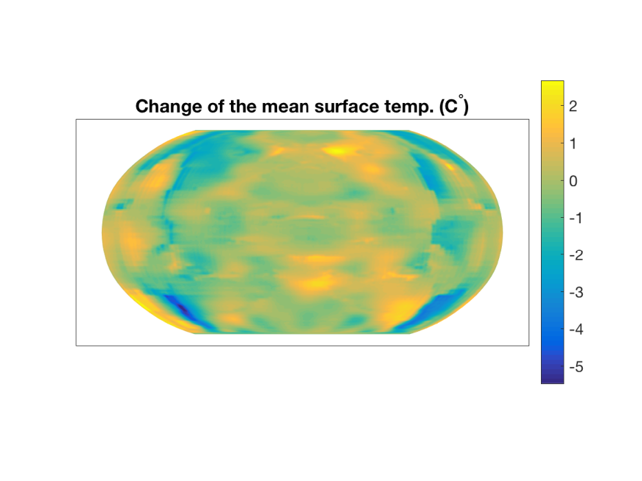
We investigate a discretization of a class of stochastic heat equations on the unit sphere with multiplicative noises. A spectral method is used for the spatial discretization and the truncation of the Wiener process, while an implicit Euler scheme with non-uniform steps is used for the temporal discretization. Some numerical experiments inspired by Earth’s surface temperature data analysis GISTEMP provided by NASA are given.

Keywords:

stochastic heat equation, multiplicative noise, non-uniform time discretization, implicit Euler scheme, isotropic random fields, sphere

1 Introduction

Let $\mathbb{S}^{2}$ be the unit sphere in the Euclidean space $\mathbb{R}^{3}$ , that is

\mathbb{S}^{2}=\{{\bf x}\in\mathbb{R}^{3}:|{\bf x}|=1\},

where $|\cdot|$ denotes the usual Euclidean norm. We consider the following stochastic heat equation

	$\displaystyle\mathrm{d}X(t)$	$\displaystyle=\Delta^{\ast}X(t)\mathrm{d}t+B(X(t))\mathrm{d}W(t),$		(1.1)
	$\displaystyle X(0)$	$\displaystyle=\xi,\qquad t\in[0,1],$		(1.1)

on the Hilbert space $H=L^{2}(\mathbb{S}^{2})$ , the space of equivalence classes of square integrable functions. Here $\xi\in H$ is the deterministic initial value, and $\Delta^{\ast}$ denotes the Laplace–Beltrami operator on $\mathbb{S}^{2}$ . Under suitable assumptions on $B$ , a mild solution $X=(X(t))_{t\in[0,1]}$ of (1.1) exists and is uniquely determined as a continuous process with values in $H$ (see, e.g., Da Prato and Zabczyk [1]).

For a bounded domain in $\mathbb{R}^{d}$ and a standard scalar Wiener process, numerical algorithms that solve general stochastic evolution equations on Hilbert spaces were constructed and analyzed first in the work of Grecksch and Kloeden [2]. Gyöngy and Nualart [3] also considered an implicit scheme for stochastic parabolic partial differential equations (PDEs) over the unit interval driven by space-time white noise. Further contributors to the problem include Allen, Novosel, and Zhang [4], Gyöngy[5], Shardlow [6] Davie and Gaines [7], Du and Zhang [8], Kloeden and Shott [9], Hausenblas [10, 11], Lord and Rougemon [12], Yan [13, 14], and Müller-Gronbach and Ritter [15, 16].

Recently, using a characterization of $Q$ -Wiener processes (where $Q$ is the covariance operator) on the sphere that has a rotationally invariant covariance as a random field at a fixed time, Lang and Schwab [17] considered a numerical scheme for a special case of (1.1) with $B(X)$ being the identity, i.e., equations with the additive noise.

In this work, we consider the equations on the sphere with the multiplicative noise. Following [17], we consider $Q$ -Wiener processes that have a rotationally invariant covariance function. A natural question arising would be whether or not the invariance propagates. Considering a class of affine noise, we derive an equation of second moment, and show a characterization of the invariance of the covariance function under rotation.

We will further study an Itô–Galerkin method when $B(X)$ is assumed to satisfy certain growth conditions, and consider a non-uniform temporal discretization, and establish a convergence rate. Our work also can be seen as an extension of the works by Müller-Gronbach and Ritter [15, 16], who proposed a discretization scheme for the heat equation on the unit cube $[0,1]^{d}$ which allow different time steps for different eigenspace of the covariance operator, to the spherical case. We remark that this is a non-trivial task. Their proofs that validate the non-uniform time step do not seem to be easily generalizable to a general Hilbert space setting: in the argument in [15, 16], the eigenfunctions of the Laplace operator on the cube with the Dirichlet condition being uniformly bounded is repeatedly used in the proof, further the integration by parts on $[0,1]$ , which uses the zero Dirichlet boundary condition, is crucial. On the sphere, we have neither of the properties. Upon the normalization to make them orthonormal on $L^{2}(\mathbb{S}^{2})$ , the magnitude of spherical harmonics, the eigenfunctions of the Laplace–Beltrami operator, grows as the degree of the polynomial goes up. Further, on the sphere, we lack a convenient first order derivative that corresponds to the usual derivative on $[0,1]$ . These difficulties are treated by exploiting the properties of spherical harmonics.

The paper is organized as follows. In Section 2, we review necessary facts on function spaces, random fields and Brownian motions on the unit sphere. In Section 3, we then introduce stochastic evolution equations on the sphere, and discuss the isotropy of the solution. Section 4 deals with the discretization of the SDEs using an Euler–Maruyama scheme. Error bounds are stated in Section 5. Finally some numerical results based on Earth’s surface temperature analysis GISTEMP data provided by NASA Goddard Institute for Space Science will be presented in Section 6.

2 Preliminaries

2.1 Spherical harmonics and function spaces

Let ${H:=}L^{2}(\mathbb{S}^{2})$ be the space of the equivalence classes of the square integrable functions on the unit sphere, which is equipped with the following standard inner product

\left\langle{f},{g}\right\rangle:=\int_{\mathbb{S}^{2}}f({\bf x})g({\bf x})\mathrm{d}\varsigma({\bf x}),

(2.1)

where $\mathrm{d}\varsigma$ is the surface measure of $\mathbb{S}^{2}$ . We write $\|f\|:=\sqrt{\left\langle{f},{f}\right\rangle}$ for $f\in L^{2}(\mathbb{S}^{2})$ . In spherical coordinates, for a point ${\bf x}\in\mathbb{S}^{2}$ , we have the parametrization

{\bf x}=(\sin\vartheta\cos\varphi,\sin\vartheta{\sin\varphi},\cos\vartheta)

for $\vartheta\in[0,\pi]$ and $\varphi\in[0,2\pi)$ , where for $\theta\in\{0,\pi\}$ we let $\varphi=0$ . Further, we let $\mathrm{d}\varsigma({\bf x})=\sin\vartheta\mathrm{d}\vartheta\mathrm{d}\varphi$ .

The space $L^{2}(\mathbb{S}^{2})$ admits the spherical harmonics as a complete orthonormal system. Spherical harmonics are the restrictions to $\mathbb{S}^{2}$ of homogeneous polynomials $Y({\bf x})$ in $\mathbb{R}^{3}$ which satisfy $\Delta Y({\bf x})=0$ , where ${\Delta}$ is the Laplace operator for functions on $\mathbb{R}^{3}$ . The space of all spherical harmonics of degree $\ell$ on $\mathbb{S}^{2}$ , denoted by $\mathcal{H}_{\ell}$ , has an orthonormal basis $\{Y_{\ell m}:m=-\ell,\ldots,\ell\},$ and $\mathrm{span}\{Y_{\ell m}:\ell\geq 0,|m|\leq\ell\}$ is dense in $L^{2}(\mathbb{S}^{2})$ .

The explicit formula for $Y_{\ell m}$ is given by

\displaystyle Y_{\ell m}(\vartheta,\varphi)=\begin{cases}{\sqrt{2}\sqrt{\frac{2\ell+1}{4\pi}\frac{(\ell-|m|)!}{(\ell+|m|)!}}P^{|m|}_{\ell}(\cos\vartheta)\sin(|m|\varphi)}&\text{for }m=-\ell,\dotsc,-1\\ {\sqrt{\frac{2\ell+1}{4\pi}}P^{0}_{\ell}(\cos\vartheta)}&\text{for }m=0\\ {\sqrt{2}\sqrt{\frac{2\ell+1}{4\pi}\frac{(\ell-m)!}{(\ell+m)!}}P^{m}_{\ell}(\cos\vartheta)\cos(m\varphi)}&\text{for }m=1,\dotsc,\ell{,}\\ \end{cases}

(2.2)

where $P^{m}_{\ell}$ is the associated Legendre polynomial of degree $\ell$ and order $m$ , given by

P^{m}_{\ell}(x)=(-1)^{m}(1-x^{2})^{m/2}\frac{d^{m}}{dx^{m}}P_{\ell}(x),\quad m\geq 0,\qquad\text{ for }\ x\in[-1,1],

where $P_{\ell}$ is the Legendre polynomial. Thus

\left\langle{Y_{\ell m}},{Y_{\ell^{\prime}m^{\prime}}}\right\rangle=\int_{\mathbb{S}^{2}}Y_{\ell m}({\bf x})Y_{\ell^{\prime}m^{\prime}}({\bf x})\mathrm{d}\varsigma({\bf x})=\delta_{\ell\ell^{\prime}}\delta_{mm^{\prime}},

where $\delta_{\ell\ell^{\prime}}$ is the Kronecker symbol.

The spherical harmonics of degree $\ell$ satisfy the following addition theorem [18]

\sum_{m=-\ell}^{\ell}Y_{\ell m}({\bf x})Y_{\ell m}({\bf y})=\frac{2\ell+1}{4\pi}P_{\ell}({\bf x}\cdot{\bf y}).

(2.3)

The spherical harmonics are the eigenfunctions of the Laplace–Beltrami operator $\Delta^{\ast}$ with eigenvalues $-\mu_{\ell}=-\ell(\ell+1)$ for $\ell=0,1,2,\dots$ . In other words,

\Delta^{\ast}Y_{\ell m}=-\mu_{\ell}Y_{\ell m}.

A more detailed discussion on spherical harmonics in $\mathbb{R}^{d+1}$ for $d\geq 2$ can be found in [18]. We define the Sobolev space $H^{1}$ on the sphere $\mathbb{S}^{2}$ as the domain of $({1-}\Delta^{\ast})^{\frac{1}{2}}$ :

H^{1}:=\left\{h\in L^{2}(\mathbb{S}^{2}):\|h\|^{2}_{H^{1}}=\sum_{\ell=0}^{\infty}\sum_{m=-\ell}^{\ell}(1+\mu_{\ell})\left\langle{h},{Y_{\ell m}}\right\rangle^{2}<\infty\right\}.

2.2 Isotropic Gaussian random fields on the sphere

In order to define Wiener processes properly on the sphere, firstly we discuss random fields defined on spheres. Random fields on spheres arise in modelling the cosmic microwave background (CMB) [19], modeling Saharan dust particles [20], feldspar particles [21], ice crystals [22] etc.

To define a random field on $\mathbb{S}^{2}$ , let $(\Omega,\mathcal{A},\mathbb{P})$ be a probability space and let $\mathcal{B}(\mathbb{S}^{2})$ be the Borel $\sigma$ -algebra of $\mathbb{S}^{2}$ with respect to the usual spherical metric topology. A $\mathcal{A}\otimes\mathcal{B}(\mathbb{S}^{2})$ -measurable mapping $T:\Omega\times\mathbb{S}^{2}\rightarrow\mathbb{R}$ is called a (product measurable) real-valued random field on the unit sphere.

A random field is called strongly isotropic if, for all $k\in\mathbb{N}$ , ${\bf x}_{1},\ldots,{\bf x}_{k}\in\mathbb{S}^{2}$ , and for all $g\in SO(3)$ , (here $SO(3)$ denotes the group of rotations on $\mathbb{S}^{2}$ ), the multivariate random variables $(T({\bf x}_{1}),\ldots,T({\bf x}_{k}))$ and $(T(g{\bf x}_{1}),\ldots,T(g{\bf x}_{k}))$ have the same law.

It is called $n$ -weakly isotropic for $n\geq 2$ if $\mathbb{E}(|T({\bf x})|^{2})<\infty$ for all ${\bf x}\in\mathbb{S}^{2}$ and if for $1\leq k\leq n$ , ${\bf x}_{1},\ldots,{\bf x}_{k}\in\mathbb{S}^{2}$ and $g\in SO(3)$ ,

\mathbb{E}(T({\bf x}_{1})\cdots T({\bf x}_{k}))=\mathbb{E}(T(g{\bf x}_{1})\cdots T(g{\bf x}_{k})).

Furthermore, it is called Gaussian if for all $k\in\mathbb{N}$ , ${\bf x}_{1},\ldots,{\bf x}_{k}$ the random variable $(T({\bf x}_{1}),\ldots,T({\bf x}_{k}))$ is multivariate Gaussian distributed, or equivalently, if $\sum_{i=1}^{k}a_{i}T({\bf x}_{i})$ is a normally distributed random variable for all $a_{i}\in\mathbb{R}$ , $i=1,\ldots,k$ for all $k\in\mathbb{N}$ .

For Gaussian random fields, we have the following characterization of the strong isotropy.

Proposition 2.1 (Proposition 5.10 in [19])

Let $T$ be a Gaussian random field on $\mathbb{S}^{2}$ . Then, $T$ is strongly isotropic if and only if T is $2$ -weakly isotropic.

The following result is immediately obtained, which was originally considered for the spherical harmonics of the complex form in [19, Theorem 5.13]. We note that the proof of [19, Theorem 5.13] relies on Theorem 5.5 in the same book, which relies on a group representation theorem and an orthonormal system in $L^{2}(\mathbb{S}^{2})$ . If we replace the complex inner product with a real one as in (2.1) and the complex spherical harmonics with real spherical harmonics, then the following theorem is obtained.

Theorem 2.1

Let $T$ be a 2-weakly isotropic random field on $\mathbb{S}^{2}$ , then the following statements hold true:

1.

$T$ satisfies

$\int_{\mathbb{S}^{2}}T({\bf x})^{2}\mathrm{d}\varsigma({\bf x})<\infty,\quad\text{{almost surely.}}$

$T$ admits a Karhunen–Loève expansion

T=\sum_{\ell=0}^{\infty}\sum_{m=-\ell}^{\ell}\alpha_{\ell m}Y_{\ell m},\qquad\alpha_{\ell m}=\int_{\mathbb{S}^{2}}T({\bf y})Y_{\ell m}\mathrm{d}\varsigma({\bf y}){,}

(2.4)

where the convergence is both in the sense of the following:

(a)

The series expansion (2.4) converges in $L^{2}(\Omega\times\mathbb{S}^{2};\mathbb{R})$ , that is,

\lim_{L\rightarrow\infty}\mathbb{E}\left(\int_{\mathbb{S}^{2}}(T({\bf y})-\sum_{\ell=0}^{L}\sum_{m=-\ell}^{\ell}\alpha_{\ell m}Y_{\ell m}({\bf y}))^{2}\mathrm{d}\varsigma({\bf y})\right)=0.

(b)

The series expansion (2.4) converges in $L^{2}(\Omega;\mathbb{R})$ for all ${\bf x}\in\mathbb{S}^{2}$ , i.e.,

\lim_{L\rightarrow\infty}\mathbb{E}\left((T({\bf x})-\sum_{\ell=0}^{L}\sum_{m=-\ell}^{\ell}\alpha_{\ell m}Y_{\ell m}({\bf x}))^{2}\right)=0,\quad\text{{for all ${\bf x}\in\mathbb{S}^{2}$.}}

Let $T$ be a strongly isotropic random field on $\mathbb{S}^{2}$ , then by adapting Remark 6.4 and Equation (6.6) in [19] to the real spherical harmonics, the collection $\mathbb{A}=(\alpha_{\ell m},\ell\in\mathbb{N}_{0},m=-\ell,\ldots,\ell)$ are, except for $\alpha_{00}$ , centered random variables, i.e. $\mathbb{E}(\alpha_{\ell m})=0$ for all $\ell\in\mathbb{N}$ and $m=-\ell,\ldots,\ell$ . Furthermore, they are real-valued random variables that satisfy

\mathbb{E}(\alpha_{\ell m}\alpha_{\ell^{\prime}m^{\prime}})=A_{\ell}\delta_{\ell\ell^{\prime}}\delta_{mm^{\prime}},\quad\ell,\ell^{\prime}\in\mathbb{N},\;\;|m|\leq\ell,\;\;|m^{\prime}|\leq\ell^{\prime}.

(2.5)

For $\alpha_{00}$ , it holds that

\mathbb{E}(\alpha_{00}\alpha_{\ell m})=(A_{0}+\mathbb{E}({\alpha_{00}})^{2})\delta_{0\ell}\delta_{0m}.

(2.6)

The sequence of non-negative real numbers $(A_{\ell},\ell\in\mathbb{N}_{0})$ is called the angular power spectrum of $T$ . We note that $\mathbb{E}(T)=\mathbb{E}(\alpha_{00})Y_{00}=\mathbb{E}(\alpha_{00})\sqrt{\frac{1}{4\pi}}$ . Combining the results of Proposition 2.1 and Theorem 2.1 we obtain the following corollary.

Corollary 2.1

Let $T$ be a 2-weakly isotropic Gaussian random field on $\mathbb{S}^{2}$ . Then $T$ admits the Karhunen–Loève expansion

T=\sum_{\ell=0}^{\infty}\sum_{m=-\ell}^{\ell}\alpha_{\ell m}Y_{\ell m},

where $\mathbb{A}=(\alpha_{\ell m},\ell\in\mathbb{N}_{0},m=-\ell,\ldots,\ell)$ is a family of independent real-valued Gaussian random variables such that $\alpha_{\ell m}\sim\mathcal{N}(0,A_{\ell})$ for $\ell>0$ while $\alpha_{00}\sim\mathcal{N}(\mathbb{E}(T)2\sqrt{\pi},A_{0})$ .

2.3 $L^{2}(\mathbb{S}^{2})$ -valued $Q$ -Wiener process

We now define an $H$ -valued Wiener process that is an isotropic centered Gaussian random field for any fixed time $t$ .

In the following, we assume $\{A_{\ell}\}_{\ell\geq 0}$ is a given sequence of positive real numbers such that

\displaystyle\sum_{\ell=0}^{\infty}(2\ell+1)A_{\ell}<\infty.

(2.7)

Then, the covariance kernel of an isotropic centered Gaussian random field $T$ is well defined, and is given by the formula

	$\displaystyle K_{T}({\bf x},{\bf y}):=\mathbb{E}[T({\bf x})T({\bf y})]$	$\displaystyle=\sum_{\ell=0}^{\infty}A_{\ell}\sum_{m=-\ell}^{\ell}Y_{\ell m}({\bf x})Y_{\ell m}({\bf y})$		(2.8)
		$\displaystyle=\sum_{\ell=0}^{\infty}A_{\ell}\frac{2\ell+1}{4\pi}P_{\ell}({\bf x}\cdot{\bf y}),$		(2.8)

which in turn ensures the existence of Gaussian random fields, see for example [23, 24].

Let $Q\colon H\to H$ be the integral operator associated with the covariance kernel (2.8), that is, for an element $f\in H$ ,

Qf({\bf x})=\int_{\mathbb{S}^{2}}K_{T}({\bf x},{\bf y})f({\bf y})\mathrm{d}\varsigma({\bf y}),\quad{\bf x}\in\mathbb{S}^{2}.

Then, we see that

	$\displaystyle QY_{L,M}({\bf x})$	$\displaystyle=\int_{\mathbb{S}^{2}}K_{T}({\bf x},{\bf y})Y_{L,M}({\bf y})\mathrm{d}\varsigma{({\bf y})}$
		$\displaystyle=A_{L}Y_{L,M}({\bf x}),\quad L=0,1,2,\ldots;\|M\|\leq L.$

and thus from (2.7) $Q$ is of trace class with $\mathrm{Tr}(Q)=\sum_{\ell=0}^{\infty}(2\ell+1)A_{\ell}<\infty$ . The $Q$ -Wiener process taking values in $H$ can be characterized by the Karhunen–Loève expansion

W(t,{\bf x})=\sum_{\ell=0}^{\infty}\sum_{m=-\ell}^{\ell}\alpha_{\ell m}(t)Y_{\ell m}({\bf x}),

(2.9)

where $\{\alpha_{\ell m}\}$ is given by

\displaystyle\alpha_{\ell m}(t):=\sqrt{A}_{\ell}w_{\ell m}(t),

(2.10)

where $\{w_{\ell m}\}$ is a system of independent standard Brownian motions that are adapted to the underlying filtration with the usual condition. From this representation, we see that the corresponding $Q$ -Wiener process satisfies the following: for any $t\in[0,1]$ the random field $W(t,\cdot)$ is an isotropic centered Gaussian random field:

\displaystyle\mathbb{E}[W(t,{\bf x})W(t,{\bf y})]=tK_{T}({\bf x},{\bf y}).

(2.11)

3 Stochastic evolution equations on the sphere

3.1 Existence and uniqueness

In the following, $\alpha\preceq\beta$ means that $\alpha$ can be bounded by some constant times $\beta$ uniformly with respect to any parameters on which $\alpha$ and $\beta$ may depend. Further, $\alpha\asymp\beta$ means that $\alpha\preceq\beta$ and $\beta\preceq\alpha$ .

In order to define stochastic integrals with respect to the $Q$ -Wiener process defined in the previous section, we introduce the Hilbert space

H_{0}=Q^{1/2}(H),

equipped with the inner product

{\left\langle{h_{1}},{h_{2}}\right\rangle_{H_{0}}=\sum_{\ell=0}^{\infty}\sum_{m=-\ell}^{\ell}{\frac{1}{A}_{\ell}}\left\langle{h_{1}},{Y_{\ell m}}\right\rangle\left\langle{h_{2}},{Y_{\ell m}}\right\rangle,\quad\text{for $h_{1},h_{2}\in H_{0}$}.}

We note $\{\sqrt{A_{\ell}}Y_{\ell m}\}$ forms a complete orthonormal system in $H_{0}$ .

Let $(S(t))_{t\geq 0}$ be the strongly continuous operator semigroup acting on $H$ generated by $\Delta^{\ast}$ . Then, we have the spectral representation

S(t)u:=\sum_{\ell=0}^{\infty}\sum_{m=-\ell}^{\ell}\exp(-\mu_{\ell}t)\left\langle{u},{Y_{\ell m}}\right\rangle Y_{\ell m}\qquad\text{ for }\ u\in H.

See, for example [25].

Let $\mathcal{L}=\mathcal{L}_{2}(H_{0},H)$ be the space of Hilbert–Schmidt operators from $H_{0}$ to $H$ , and $\|\cdot\|_{\mathcal{L}}$ denote the Hilbert–Schmidt norm. We assume that $B$ is Lipschitz continuous in the following sense:

{\|B(u)-B(v)\|_{\mathcal{L}}\leq C_{\mathrm{Lip}}\|u-v\|\quad\text{ for }\quad u,v\in H,}

(3.1)

and $B$ satisfies the following linear growth condition:

\displaystyle{\|B(u)\|_{\mathcal{L}}\leq c(1+\|u\|),\quad\text{ for }\quad u\in H,}

(3.2)

for some positive constant $c$ . In particular, $B\colon H\rightarrow\mathcal{L}$ is $\mathcal{B}(H)/\mathcal{B}(\mathcal{L})$ -measurable.

In this work, we restrict our consideration to the operators $B$ of the form

\displaystyle B(u)h=T_{g}(u)\cdot\widetilde{B}h,\text{ for }u\in H,\quad h\in H_{0},

(3.3)

where $T_{g}\colon H\to H$ is the Nemytskii operator

{T_{g}(u)({\bf x}):=g(u({\bf x})),\qquad\text{for }u\in H,\quad{\bf x}\in\mathbb{S}^{2},}

with $g\in C^{1}(\mathbb{R})$ such that $\|g^{\prime}\|_{\infty}:=\sup_{r\in\mathbb{R}}|g^{\prime}(r)|<\infty$ , and $\widetilde{B}\colon{H_{0}}\to H$ is given by

\displaystyle{\widetilde{B}h:=\sum_{\ell=0}^{\infty}\sum_{m=-\ell}^{\ell}\eta_{\ell m}\left\langle{h},{Y_{\ell m}}\right\rangle Y_{\ell m},}

(3.4)

with $\{\eta_{\ell m}\}\subset\mathbb{R}$ such that $\sup_{\ell,m}|\eta_{\ell m}|<\infty$ . We note that for $u\in H$ we indeed have $T_{g}(u)\in H$ , as

\displaystyle\|T_{g}(u)\|\leq\int_{\mathbb{S}^{2}}\big(2|g(0_{H}({\bf x}))|^{2}+2\|g^{\prime}\|_{\infty}^{2}|u({\bf x})|^{2}\big)\mathrm{d}\varsigma({\bf x})\preceq 1+\|u\|.

(3.5)

This generalizes [16], where $\widetilde{B}:=I$ was considered. We also note for $u,v\in H$ we have

\displaystyle{\|T_{g}(u)-T_{g}(v)\|\leq\|g^{\prime}\|_{\infty}\|u-v\|.}

(3.6)

Such $B$ satisfies the aforementioned conditions: for $u\in H$ we have

$\displaystyle\\|$	$\displaystyle B(u)\\|_{\mathcal{L}(H_{0},H)}^{2}=\sum_{\ell=0}^{\infty}\sum_{m=-\ell}^{\ell}\int_{\mathbb{S}^{2}}\big\|g(u({\bf x})){\eta_{\ell m}}\sqrt{A_{\ell}}Y_{{\ell m}}({\bf x})\big\|^{2}\mathrm{d}\varsigma({\bf x})$	(3.7)
	$\displaystyle\leq{\Big(\sup_{\lambda,\nu}\|\eta_{\lambda\nu}\|\Big)^{2}}\sum_{\ell=0}^{\infty}A_{\ell}\int_{\mathbb{S}^{2}}\big(2\|g(0_{H}({\bf x}))\|^{2}+2\\|g^{\prime}\\|_{\infty}^{2}\|u({\bf x})\|^{2}\big)\sum_{m=-\ell}^{\ell}Y_{\ell m}({\bf x})Y_{\ell m}({\bf x})\mathrm{d}\varsigma({\bf x})$	(3.8)
	$\displaystyle=\frac{{\Big(\sup_{\lambda,\nu}\|\eta_{\lambda\nu}\|\Big)^{2}}}{4\pi}\sum_{\ell=0}^{\infty}A_{\ell}(2\ell+1)\big(8\pi\|g(0)\|^{2}+2\\|g^{\prime}\\|_{\infty}^{2}\\|u\\|_{H}^{2}\big)<\infty.$	(3.9)

Further, for $u,v\in H$ we have

$\displaystyle\\|$	$\displaystyle B(u)-B(v)\\|_{\mathcal{L}(H_{0},H)}^{2}=\sum_{\ell=0}^{\infty}\sum_{m=-\ell}^{\ell}\int_{\mathbb{S}^{2}}\big\|\big(g(u({\bf x}))-g(v({\bf x}))\big){\eta_{\ell m}}\sqrt{A_{\ell}}Y_{{\ell m}}({\bf x})\big\|^{2}\mathrm{d}\varsigma({\bf x})$	(3.10)
	$\displaystyle\leq{\Big(\sup_{\lambda,\nu}\|\eta_{\lambda\nu}\|\Big)^{2}}\\|g^{\prime}\\|_{\infty}\sum_{\ell=0}^{\infty}A_{\ell}\int_{\mathbb{S}^{2}}\|u({\bf x})-v({\bf x})\|^{2}\sum_{m=-\ell}^{\ell}Y_{\ell m}({\bf x})Y_{\ell m}({\bf x})\mathrm{d}\varsigma({\bf x})$	(3.11)
	$\displaystyle={\Big(\sup_{\lambda,\nu}\|\eta_{\lambda\nu}\|\Big)^{2}}\frac{\\|g^{\prime}\\|_{\infty}}{{4\pi}}\sum_{\ell=0}^{\infty}A_{\ell}{(2\ell+1)}\\|u-v\\|_{H}^{2},$	(3.12)

and thus the Lipschitz constant in (3.1) is the square root of

\displaystyle C_{\mathrm{Lip}}^{2}:=\mathrm{Tr}Q\frac{\|g^{\prime}\|_{\infty}}{{4\pi}}{\Big(\sup_{\lambda,\nu}|\eta_{\lambda\nu}|\Big)^{2}}.

(3.13)

Examples of $g$ are ${T_{g}}(u)=au+b$ for some given real numbers $a,b$ . We recall the following existence and uniqueness results for the solution from [1, Section 7.1], which is applicable to our problem.

Theorem 3.1

Under the assumptions that $B$ is Lipschitz and satisfies the linear growth condition, there exists an continuous process $(X(t))_{t\in[0,1]}$ with values in $H$ which is adapted to the underlying filtration such that

X(t)=S(t)\xi+\int_{0}^{t}S(t-s){B(X(s))}\mathrm{d}W(s),\quad t\in[0,1]\quad\text{$\mathbb{P}$-a.s.}

(3.14)

Moreover, this process is uniquely determined $\mathbb{P}$ -a.s., and it is called the mild solution of the stochastic evolution equation

\mathrm{d}X(t)=\Delta^{\ast}X(t)\mathrm{d}t+{B(X(t))}\mathrm{d}W(t),\quad X(0)=\xi.

For $p\geq 1$ ,

\sup_{t\in[0,T]}\mathbb{E}\|X(t)\|^{p}<\infty.

(3.15)

Let

X(t)={\sum_{\ell=0}^{\infty}\sum_{m=-\ell}^{\ell}}X_{\ell m}(t)Y_{\ell m},\quad X_{\ell m}(t)=\left\langle{X(t)},{Y_{\ell m}}\right\rangle,

(3.16)

for $\ell\in\mathbb{N}_{0}$ . The processes $X_{\ell m}=(X_{\ell m}(t))_{t\in[0,1]}$ satisfy the following bi-infinite system of stochastic differential equations

	$\displaystyle\mathrm{d}X_{\ell m}(t)$	$\displaystyle=-\mu_{\ell}X_{\ell m}(t)\mathrm{d}t+\sum_{\ell^{\prime}=0}^{\infty}\sum_{m^{\prime}=-\ell^{\prime}}^{\ell^{\prime}}\sqrt{A_{\ell^{\prime}}}\left\langle{B(X(t))Y_{\ell^{\prime}m^{\prime}}},{Y_{\ell m}}\right\rangle\mathrm{d}w_{\ell^{\prime}m^{\prime}}(t)$
	$\displaystyle X_{\ell m}(0)$	$\displaystyle=\left\langle{\xi},{Y_{\ell m}}\right\rangle,\qquad\ell\in\mathbb{N}_{0},\;m=-\ell,\ldots,\ell.$

Each process $X_{\ell m}$ is given explicitly as

X_{\ell m}(t)=\exp(-\mu_{\ell}t)\left\langle{\xi},{Y_{\ell m}}\right\rangle+\sum_{\ell^{\prime}=0}^{\infty}\sum_{m^{\prime}=-\ell^{\prime}}^{\ell^{\prime}}\sqrt{A_{\ell^{\prime}}}Z_{\ell m,\ell^{\prime}m^{\prime}}(t),

(3.17)

where

Z_{\ell m,\ell^{\prime}m^{\prime}}(t)=\int_{0}^{t}\exp(-\mu_{\ell}(t-s))\left\langle{B(X(s))Y_{\ell^{\prime}m^{\prime}}},{Y_{\ell m}}\right\rangle\mathrm{d}w_{\ell^{\prime}m^{\prime}}(s).

(3.18)

We note that the series $\sum_{\ell^{\prime}=0}^{\infty}\sum_{m^{\prime}=-\ell^{\prime}}^{\ell^{\prime}}\sqrt{A_{\ell^{\prime}}}Z_{\ell m,\ell^{\prime}m^{\prime}}(t)$ in the second term is convergent in $L^{2}(\Omega)$ , due to (3.2) and (3.15).

3.2 Temporal regularity

The following regularity estimate will be used for the spatial truncation error estimate, see Theorem 5.1. A similar result for the stochastic PDE defined on $[0,1]^{d}$ with the Dirichlet condition was proved in [15]. In the same spirit, we prove the following regularity result for the stochastic PDE defined on the unit sphere. See also [1, Theorem 9.1] for the mean-square continuity of the solution.

Lemma 3.1

Suppose the Lipschitz condition (3.1) and the linear growth condition (3.2) are satisfied. Then, the mild solution is continuous in the mean-square sense on $[0,1]$ . Further, we have the estimate

\mathbb{E}\|X(s)-X(t)\|^{2}\leq C|t-s|(1+\psi(\min\{s,t\})),

where $\psi\in L_{1}([0,1])$ .

Proof First, note that we have

\mathbb{E}\|X(s)-X(t)\|^{2}=\sum_{\ell=0}^{\infty}\sum_{m=-\ell}^{\ell}\mathbb{E}(X_{\ell m}(s)-X_{\ell m}(t))^{2}.

For $s<t$ , from (3.17) and (3.18) we have the identity

	$\displaystyle X_{\ell m}(t)-X_{\ell m}(s)$	$\displaystyle={[\exp(-\mu_{\ell}(t-s))-1]}X_{\ell m}(s)$
		$\displaystyle+\sum_{\ell^{\prime}=0}^{\infty}\sum_{m^{\prime}=-\ell^{\prime}}^{\ell^{\prime}}\int_{s}^{t}\exp(-\mu_{\ell}(t-r))\sqrt{A_{\ell^{\prime}}}\left\langle{B(X(r))Y_{\ell^{\prime}m^{\prime}}},{Y_{\ell m}}\right\rangle\mathrm{d}w_{\ell^{\prime}m^{\prime}}(r),$

By the Itô’s isometry, we have

	$\displaystyle\mathbb{E}(X_{\ell m}(s)-X_{\ell m}(t))^{2}$	$\displaystyle={[\exp(-\mu_{\ell}(t-s))-1]^{2}}\mathbb{E}(X^{2}_{\ell m}(s))$
		$\displaystyle+\int_{s}^{t}\exp(-2\mu_{\ell}(t-r))\mathbb{E}\\|B^{*}(X(r))Y_{\ell m}\\|^{2}_{H_{0}}\mathrm{d}r,$

with

\displaystyle\|B^{*}(X)Y_{\ell,m}\|_{H_{0}}^{2}=\sum_{\ell^{\prime}=0}A_{\ell^{\prime}}\sum_{|m^{\prime}|\leq\ell^{\prime}}|\left\langle{B(X)Y_{\ell^{\prime}m^{\prime}}},{Y_{\ell m}}\right\rangle|^{2}{,}

(3.19)

where $B^{*}(x):=(B(x))^{*}\colon H\to H_{0}$ for $x\in H$ denotes the adjoint operator of $B(x)$ . Similarly, we also have

	$\displaystyle\mathbb{E}(X_{\ell m}(s))^{2}$	$\displaystyle=\exp(-2\mu_{\ell}s)\left\langle{\xi},{Y_{\ell m}}\right\rangle^{2}$		(3.20)
		$\displaystyle+\int_{0}^{s}\exp(-2\mu_{\ell}(s-r))\mathbb{E}\\|B^{*}(X(r))Y_{\ell m}\\|^{2}_{H_{0}}\mathrm{d}r.$		(3.20)

Put

\Gamma_{1}=\sum_{\ell=0}^{\infty}\sum_{m=-\ell}^{\ell}{[\exp(-\mu_{\ell}(t-s))-1]^{2}}\mathbb{E}(X_{\ell m}^{2}(s))

and

\Gamma_{2}=\sum_{\ell=0}^{\infty}\sum_{m=-\ell}^{\ell}\int_{s}^{t}\exp(-2\mu_{\ell}(t-r))\mathbb{E}\|B^{*}(X(r))Y_{\ell m}\|^{2}_{H_{0}}\mathrm{d}r.

We use (3.15) and the linear growth condition to obtain

	$\displaystyle\Gamma_{2}$	$\displaystyle\leq\mathbb{E}\bigg(\int_{s}^{t}\sum_{\ell=0}^{\infty}\sum_{m=-\ell}^{\ell}\\|B^{*}(X(r))Y_{\ell m}\\|_{H_{0}}^{2}{\mathrm{d}r}\bigg)$		(3.21)
		$\displaystyle=\mathbb{E}\bigg(\int_{s}^{t}\\|B^{*}(X(r))\\|^{2}_{\mathcal{L}(H,H_{0})}{\mathrm{d}r}\bigg)\leq C(t-s).$		(3.21)

Fix $\varepsilon>0$ arbitrarily. Then, for sufficiently large $L_{0}$ we have

\sup_{s\in[0,1]}\sum_{\ell=L_{0}+1}^{\infty}\sum_{m=-\ell}^{\ell}\mathbb{E}(X_{\ell m}^{2}(s))<\frac{\varepsilon}{2}.

Further, we can take $\delta>0$ such that for any $|t-s|<\delta$ and for any $1\leq\ell\leq L_{0}$ we have

[\exp(-\mu_{\ell}(t-s))-1]^{2}\mathbb{E}(X_{\ell m}^{2}(s))<\frac{\varepsilon}{2L_{0}}.

Thus, for such $s,t$ we have $\Gamma_{1}\leq\varepsilon$ , and thus together with (3.21) the mean square continuity follows.

Now, since $1-\exp(-x){\leq x}$ we have ${\Gamma_{1}\leq\sum_{\ell=0}^{\infty}\mu_{\ell}(t-s)\mathbb{E}(X_{\ell m}^{2}(s))}$ , where the series is well defined since each term is non-negative. Therefore, $\Gamma_{1}\leq(t-s)\psi(s)$ with

\psi(s):=\sum_{\ell=0}^{\infty}\sum_{m=-\ell}^{\ell}\mu_{\ell}\mathbb{E}(X^{2}_{\ell m}(s)).

Since

\displaystyle\mu_{\ell}\int_{0}^{1}\mathbb{E}(X^{2}_{\ell m}(s))\mathrm{d}s\leq\left\langle{\xi},{Y_{\ell m}}\right\rangle^{2}+\int_{0}^{1}\mathbb{E}\|B^{*}(X(r))Y_{\ell m}\|^{2}_{H_{0}}\mathrm{d}r

(3.22)

we have

\psi\in L_{1}([0,1]).

(3.23)

$\Box$

3.3 Isotropy of the solution

The equation (1.1) is driven by the Wiener process that is 2-weakly isotropic at each $t$ . Thus, whether or not the isotropy propagates to the solution is of natural interest. In this section, we see that the solution does not necessarily have the isotropy in general. To see this, in this section we consider the Nemytskii operator $T_{g}$ with affine functions $g(x)=ax+b$ , for some $a,b\in\mathbb{R}$ .

We start from the following relation between the 2-weak isotropy and the eigenvalues of covariance operators.

Proposition 3.1

Let $Z=\{Z({\bf x})\}_{{\bf x}\in\mathbb{S}^{2}}$ be a zero-mean random field on $\mathbb{S}^{2}$ such that its covariance function $K_{Z}(\cdot,\cdot)\colon\mathbb{S}^{2}\times\mathbb{S}^{2}\to\mathbb{R}$ is well-defined on all points $\mathbb{S}^{2}\times\mathbb{S}^{2}$ , and $Z$ is $\mathcal{B}(\mathbb{S}^{2})\otimes\mathscr{F}/\mathcal{B}(\mathbb{R})$ -measurable. Then, $Z$ is $2$ -weakly isotropic if and only if $K_{Z}\in L^{2}(\mathbb{S}^{2}\times\mathbb{S}^{2})$ and the covariance operator $Q_{Z}$ defined as the integral operator

H\ni h\mapsto Q_{Z}h:=\int_{\mathbb{S}^{2}}K_{Z}(\cdot,{\bf x})h({\bf x})\mathrm{d}\varsigma({\bf x})\in H

has eigenfunctions $\{Y_{\ell m};{\ell\in\mathbb{N}_{0},m=-\ell,\ldots,\ell\}}$ with eigenvalues independent of $m$ .

Proof Since $Z$ is $2$ -weakly isotropic, letting ${\bf x}_{\mathrm{n}}$ be the north pole we have $K_{Z}\in L^{2}(\mathbb{S}^{2}\times\mathbb{S}^{2})$ :

	$\displaystyle\int_{\mathbb{S}^{2}}\!\!\int_{\mathbb{S}^{2}}\|K_{Z}({\bf x}_{1},{\bf x}_{2})\|^{2}\mathrm{d}\varsigma({\bf x}_{1})\mathrm{d}\varsigma({\bf x}_{2})$	$\displaystyle\leq\int_{\mathbb{S}^{2}}\!\!\int_{\mathbb{S}^{2}}\|\mathbb{E}[Z({\bf x}_{1})^{2}]\|\|\mathbb{E}[Z({\bf x}_{2})^{2}]\|\mathrm{d}\varsigma({\bf x}_{1})\mathrm{d}\varsigma({\bf x}_{2})$		(3.24)
		$\displaystyle=16\pi^{2}\|\mathbb{E}[Z({\bf x}_{\mathrm{n}})^{2}]\|^{2}<\infty.$		(3.25)

Thus we have the expansion of $K_{Z}$ as

\displaystyle K_{Z}({\bf x}_{1},{\bf x}_{2})=\sum_{\ell=0}^{\infty}\frac{2\ell+1}{4\pi}A_{\ell}P_{\ell}({\bf x}_{1}\cdot{\bf x}_{2})=\sum_{\ell=0}^{\infty}\sum_{m=-\ell}^{\ell}A_{\ell}Y_{\ell m}({\bf x}_{1})Y_{\ell m}({\bf x}_{2}),

(3.26)

with some sequence $\{A_{\ell}\}$ , where in the second equality the addition theorem is used. Thus, we immediately see $Q_{Z}$ has the eigenpair $(A_{\ell},Y_{\ell m})$ . Conversely, if we have $K_{Z}\in L^{2}(\mathbb{S}^{2}\times\mathbb{S}^{2})$ , then we have the representation

K_{Z}({\bf x}_{1},{\bf x}_{2})=\sum_{\lambda=0}^{\infty}\sum_{\nu=-\lambda}^{\lambda}\sum_{\lambda^{\prime}=0}^{\infty}\sum_{\nu^{\prime}=-\lambda^{\prime}}^{\lambda^{\prime}}C_{\lambda\nu\lambda^{\prime}\nu^{\prime}}Y_{\lambda\nu}({\bf x}_{1})Y_{\lambda^{\prime}\nu^{\prime}}({\bf x}_{2}),

for some $\{C_{\ell m\ell^{\prime}m^{\prime}}\}$ in $L^{2}(\mathbb{S}^{2}\times\mathbb{S}^{2})$ . From the assumption we have

Q_{Z}Y_{\ell m}=\int_{\mathbb{S}^{2}}K_{Z}(\cdot,{\bf x})Y_{\ell m}({\bf x})\mathrm{d}\varsigma({\bf x})=A_{\ell}Y_{\ell m},

thus $\sum_{\lambda=0}^{\infty}\sum_{\nu=-\lambda}^{\lambda}C_{\lambda\nu\ell m}Y_{\lambda\nu}=A_{\ell}Y_{\ell m}$ . Multiplying $\{Y_{\ell m}\}$ to both sides and integrating over $\mathbb{S}^{2}$ yields $C_{\ell m\ell m}=A_{\ell}$ and $C_{\lambda\nu\ell m}=0$ unless $\lambda=\ell$ and $\nu=m$ . $\Box$

From the previous result, we expect that the isotropy should be preserved as long as the isotropic noise $W$ is acted upon by operators that are diagonalised by $\{Y_{\ell,m}\}$ and their eigenvalues do not depend on $m$ ’s. Now, we note that the mapping $B$ is defined by the pointwise multiplication and a Nemytskij operator. This makes the analysis difficult, because non-trivial multiplication operators cannot be diagonalised by $\{Y_{\ell,m}\}$ as we see in the next proposition.

Let $f\in H$ and the multiplication operator $\mathscr{M}_{f}\colon H_{0}\to H$ be defined by

(\mathscr{M}_{f}h)({\bf x})=f({\bf x})h({\bf x})\quad\text{ for }h\in H_{0}.

Proposition 3.2

Suppose $f\in{H}$ defines a multiplication operator such that $\mathscr{M}_{f}\in\mathcal{L}$ . Suppose further that $f$ is not a constant function on $\mathbb{S}^{2}$ . Then, $\mathscr{M}_{f}$ cannot be diagonalised by $\{Y_{\ell m}\}$ . In particular, $\mathscr{M}_{f}$ cannot not have $\{Y_{\ell m}\}$ as eigenfunctions.

Proof

Suppose the $\mathscr{M}_{f}$ can be diagonalised by $Y_{\ell m}$ , i.e., for $h\in H$ we have $\mathscr{M}_{f}h=fh=\sum_{\ell=0}^{\infty}\sum_{m=-\ell}^{\ell}c_{\ell m}\left\langle{h},{Y_{\ell m}}\right\rangle Y_{\ell m}$ with some $\{c_{\ell m}\}\subset\mathbb{R}$ . In particular, we have $(\mathscr{M}_{f}h)({\bf x})=f({\bf x})Y_{\lambda\nu}({\bf x})=c_{\lambda\nu}Y_{\lambda\nu}({\bf x}).$ For all $\lambda>1$ , $\nu=-\lambda,\dots,\lambda$ , integrating both sides over $\mathbb{S}^{2}$ yields

\displaystyle\int_{\mathbb{S}^{2}}f({\bf x})Y_{\lambda\nu}({\bf x})\mathrm{d}\varsigma({\bf x})=0.

(3.27)

Thus, we must have $f\in\mathrm{span}\{Y_{00}\}$ , which contradicts the assumption. $\Box$

3.3.1 Equations for the second moment

To study the propagation of 2-weak isotropy, we formulate the equations for the second moment—the equation that has the covariance function of the solution $X$ as the solution—as an abstract Cauchy problem in $L^{2}(\mathbb{S}^{2}\times\mathbb{S}^{2})$ .

In the following we assume the initial condition $\xi$ is constant over $\mathbb{S}^{2}$ so that the deterministic random field $\xi$ is 2-weakly isotropic.

Let $S\diamond BW:=\int_{0}^{\cdot}S(t-s){B}(X(s))\mathrm{d}W(s)$ . Then, $X(t)=S(t)\xi+(S\diamond BW)(t)\in H$ , and $\mathbb{E}[S\diamond BW]=0$ . Since $\mathbb{E}[X(t)]=S(t)\xi$ , we see that $\mathbb{S}^{2}\ni{\bf x}\mapsto\mathbb{E}[X(t,{\bf x})]$ is a constant function given that $\xi$ is constant over $\mathbb{S}^{2}$ . Thus, to show the 2-weak isotropy of $X(t,\cdot)$ , it suffices to show that for any fixed $t>0$ the covariance of $X(t,{\bf x}_{1})$ and $X(t,{\bf x}_{2})$ is rotationally invariant for any ${\bf x}_{1},{\bf x}_{2}\in\mathbb{S}^{2}$ .

We start with the following formula.

Lemma 3.2

For any $\ell,\ell^{\prime}\geq 0$ , $|m|\leq\ell$ , $|m^{\prime}|\leq\ell^{\prime}$ , we have

		$\displaystyle\mathbb{E}\Big[\big\langle X(t)-S(t)\xi,Y_{\ell m}\big\rangle\big\langle X(t)-S(t)\xi,Y_{\ell^{\prime}m^{\prime}}\big\rangle\Big]$
		$\displaystyle=\sum_{\lambda=0}^{\infty}\sum_{\nu=-\lambda}^{\lambda}\mathbb{E}\bigg[\int_{0}^{t}\left\langle{\sqrt{A}_{\lambda}S(t-s)B(X(s))Y_{\lambda\nu}},{Y_{\ell m}}\right\rangle\left\langle{\sqrt{A}_{\lambda}S(t-s)B(X(s))Y_{\lambda\nu}},{Y_{\ell^{\prime}m^{\prime}}}\right\rangle\mathrm{d}s\bigg].$		(3.28)

Proof Since $X(t)=S(t)\xi+\int_{0}^{t}S(t-s){B}(X(s))\mathrm{d}W(s)$ , we have that for any $h\in H$

\displaystyle\big\langle X(t)-S(t)\xi,h\big\rangle=\sum_{\lambda=0}^{\infty}\sum_{\nu=-\lambda}^{\lambda}\int_{0}^{t}\left\langle{\sqrt{A}_{\lambda}S(t-s)B(X(s))Y_{\lambda\nu}},{h}\right\rangle\mathrm{d}w_{\lambda\nu}(s),

(3.29)

with the series convergent in $L^{2}(\Omega)$ .

Since $\{w_{\lambda\nu}\}$ are independent standard Brownian motions and thus their quadratic covariations vanish unless the indices $\lambda$ and $\nu$ coincide, the Itô’s isometry implies

		$\displaystyle\mathbb{E}\bigg[\int_{0}^{t}\left\langle{\sqrt{A}_{\lambda}S(t-s)B(X(s))Y_{\lambda\nu}},{h}\right\rangle\mathrm{d}w_{\lambda\nu}(s)\int_{0}^{t}\left\langle{\sqrt{A}_{\lambda^{\prime}}S(t-s)B(X(s))Y_{\lambda^{\prime}\nu^{\prime}}},{h^{\prime}}\right\rangle\mathrm{d}w_{\lambda^{\prime}\nu^{\prime}}(s)\bigg]$
		$\displaystyle=\delta_{\lambda\lambda^{\prime}}\delta_{\nu\nu^{\prime}}\mathbb{E}\bigg[\int_{0}^{t}\left\langle{\sqrt{A}_{\lambda}S(t-s)B(X(s))Y_{\lambda\nu}},{h}\right\rangle\left\langle{\sqrt{A}_{\lambda}S(t-s)B(X(s))Y_{\lambda\nu}},{h^{\prime}}\right\rangle\mathrm{d}s\bigg].$		(3.30)

From these two facts we have

		$\displaystyle\mathbb{E}\Big[\big\langle X(t)-S(t)\xi,Y_{\ell m}\big\rangle\big\langle X(t)-S(t)\xi,Y_{\ell^{\prime}m^{\prime}}\big\rangle\Big]$
		$\displaystyle=\sum_{\lambda=0}^{\infty}\sum_{\nu=-\lambda}^{\lambda}\mathbb{E}\bigg[\int_{0}^{t}\left\langle{\sqrt{A}_{\lambda}S(t-s)B(X(s))Y_{\lambda\nu}},{Y_{\ell m}}\right\rangle\left\langle{\sqrt{A}_{\lambda}S(t-s)B(X(s))Y_{\lambda\nu}},{Y_{\ell^{\prime}m^{\prime}}}\right\rangle\mathrm{d}s\bigg],$

which completes the proof. $\Box$

Now we assume $g(x)=x$ for $x\in\mathbb{R}$ . That is, $(B(u)h)({\bf x})=u({\bf x})(\widetilde{B}h)({\bf x})$ . Noting that $\sup_{s\in[0,1]}\|X(s)\|^{2}<\infty$ , we have

		$\displaystyle\mathbb{E}\Big[\big\langle X(t)-S(t)\xi,Y_{\ell m}\big\rangle\big\langle X(t)-S(t)\xi,Y_{\ell^{\prime}m^{\prime}}\big\rangle\Big]$
		$\displaystyle=\mathbb{E}\Big[\big\langle X(t),Y_{\ell m}\big\rangle\big\langle X(t),Y_{\ell^{\prime}m^{\prime}}\big\rangle\Big]-\big\langle S(t)\xi,Y_{\ell m}\big\rangle\big\langle S(t)\xi,Y_{\ell^{\prime}m^{\prime}}\big\rangle$
		$\displaystyle=\int_{\mathbb{S}^{2}}\!\!\int_{\mathbb{S}^{2}}\mathbb{E}\int_{0}^{t}[X(t,{\bf x}_{1})X(t,{\bf x}_{2})]Y_{\ell m}({\bf x}_{1})Y_{\ell^{\prime}m^{\prime}}({\bf x}_{2})\mathrm{d}s\mathrm{d}\varsigma({\bf x}_{1})\mathrm{d}\varsigma({\bf x}_{2})$
		$\displaystyle\phantom{==}-\int_{\mathbb{S}^{2}}\!\!\int_{\mathbb{S}^{2}}S(t)\xi({\bf x}_{1})\cdot S(t)\xi({\bf x}_{2})Y_{\ell m}({\bf x}_{1})Y_{\ell^{\prime}m^{\prime}}({\bf x}_{2})\mathrm{d}\varsigma({\bf x}_{1})\mathrm{d}\varsigma({\bf x}_{2}),$		(3.31)

where in the first equality we used that $\mathbb{E}\langle X(t),Y_{\ell^{\prime}m^{\prime}}\rangle=\langle S(t)\xi,Y_{\ell^{\prime}m^{\prime}}\rangle$ .

Further, since $\big\langle{\sqrt{A}_{\lambda}S(t-s)B(X(s))Y_{\lambda\nu}},{Y_{\ell m}}\big\rangle=\big\langle{\sqrt{A}_{\lambda}X(s)\mathrm{e}^{-\mu_{\lambda}(t-s)}\eta_{\lambda\nu}Y_{\lambda\nu}},{Y_{\ell m}}\big\rangle$ , we have

\displaystyle\big\langle{|\sqrt{A}_{\lambda}S(t-s)B(X(s))Y_{\lambda\nu}|},{|Y_{\ell m}|}\big\rangle\leq c\sqrt{2\ell+1}\sup_{s\in[0,1]}\|X(s)\|\sqrt{A}_{\lambda}{\mathrm{e}^{-\mu_{\lambda}(t-s)}}{\sqrt{2\lambda+1}}\eta_{\lambda\nu}<\infty.

Noting $\sum_{\lambda=0}^{\infty}\sum_{\nu=-\lambda}^{\lambda}{A}_{\lambda}(2\lambda+1)\int_{0}^{t}{\mathrm{e}^{-2\mu_{\lambda}(t-s)}}\mathrm{d}s\leq\sum_{\lambda=0}^{\infty}\sum_{\nu=-\lambda}^{\lambda}{A}_{\lambda}\frac{2\lambda+1}{\mu_{\lambda}}<\infty$ , together with $\sup_{\lambda,\nu}|\eta_{\lambda\nu}|<\infty$ we can rewrite (3.28) by changing the order of the integrals as

		$\displaystyle\int_{\mathbb{S}^{2}}\!\!\int_{\mathbb{S}^{2}}\mathbb{E}[X(t,{\bf x}_{1})X(t,{\bf x}_{2})]Y_{\ell m}({\bf x}_{1})Y_{\ell^{\prime}m^{\prime}}({\bf x}_{2})\mathrm{d}\varsigma({\bf x}_{1})\mathrm{d}\varsigma({\bf x}_{2})$
		$\displaystyle\phantom{===============}-\int_{\mathbb{S}^{2}}\!\!\int_{\mathbb{S}^{2}}S(t)\xi({\bf x}_{1})\cdot S(t)\xi({\bf x}_{2})Y_{\ell m}({\bf x}_{1})Y_{\ell^{\prime}m^{\prime}}({\bf x}_{2})\mathrm{d}\varsigma({\bf x}_{1})\mathrm{d}\varsigma({\bf x}_{2})$		(3.32)
		$\displaystyle=\int_{\mathbb{S}^{2}}\!\!\int_{\mathbb{S}^{2}}\int_{0}^{t}\sum_{\lambda=0}^{\infty}\sum_{\nu=-\lambda}^{\lambda}\!{A}_{\lambda}\mathbb{E}[X(s,{\bf x}_{1})X(s,{\bf x}_{2})]\mathrm{e}^{-2\mu_{\lambda}(t-s)}\eta_{\lambda\nu}^{2}Y_{\lambda\nu}({\bf x}_{1})Y_{\lambda\nu}({\bf x}_{2})\mathrm{d}s$
		$\displaystyle\phantom{===============}\times Y_{\ell m}({\bf x}_{1})Y_{\ell^{\prime}m^{\prime}}({\bf x}_{2})\mathrm{d}\varsigma({\bf x}_{1})\mathrm{d}\varsigma({\bf x}_{2}).$		(3.33)

This identity suggests that the kernel $({\bf x}_{1},{\bf x}_{2})\mapsto\mathbb{E}[X(s,{\bf x}_{1})X(s,{\bf x}_{2})]$ is the weak solution of an abstract Cauchy problem in $L^{2}(\mathbb{S}^{2}\times\mathbb{S}^{2})$ . Then, the rotational invariance of the covariance is nothing but this function being a zonal kernel. This motivates us to study an abstract Cauchy problem in the space of zonal kernels.

The operator $F$ defined below will be used as the forcing term for the abstract Cauchy problem we consider.

Lemma 3.3

Let (2.7) be satisfied and let

\displaystyle\kappa({\bf x}_{1},{\bf x}_{2}):=\sum_{\lambda=0}^{\infty}\sum_{\nu=-\lambda}^{\lambda}\!{A}_{\lambda}\eta_{\lambda\nu}^{2}Y_{\lambda\nu}({\bf x}_{1})Y_{\lambda\nu}({\bf x}_{2}),\quad\text{ for }{\bf x}_{1},{\bf x}_{2}\in\mathbb{S}^{2}.

(3.34)

Then, the multiplication operator $F=F_{\kappa}$ on $L^{2}(\mathbb{S}^{2}\times\mathbb{S}^{2})$ defined by

\displaystyle v({\bf x}_{1},{\bf x}_{2})\mapsto\kappa({\bf x}_{1},{\bf x}_{2})v({\bf x}_{1},{\bf x}_{2})=:Fv({\bf x}_{1},{\bf x}_{2}),\quad({\bf x}_{1},{\bf x}_{2})\in\mathbb{S}^{2}\times\mathbb{S}^{2},

(3.35)

is bounded as an operator from $L^{2}(\mathbb{S}^{2}\times\mathbb{S}^{2})$ to $L^{2}(\mathbb{S}^{2}\times\mathbb{S}^{2})$ .

Proof First, note that from the Cauchy–Schwarz inequality and the addition theorem, the condition (2.7) implies

		$\displaystyle\sup_{({\bf x}_{1},{\bf x}_{2})\in\mathbb{S}^{2}\times\mathbb{S}^{2}}\|\kappa({\bf x}_{1},{\bf x}_{2})\|\leq\sum_{\lambda=0}^{\infty}{A}_{\lambda}\sum_{\nu=-\lambda}^{\lambda}\!\Big\|\eta_{\lambda\nu}^{2}Y_{\lambda\nu}({\bf x}_{1})Y_{\lambda\nu}({\bf x}_{2})\Big\|$		(3.36)
		$\displaystyle\leq\sum_{\lambda=0}^{\infty}{A}_{\lambda}\bigg(\sum_{\nu=-\lambda}^{\lambda}\!\eta_{\lambda\nu}^{2}Y_{\lambda\nu}({\bf x}_{1})^{2}\bigg)^{\frac{1}{2}}\bigg(\sum_{\nu=-\lambda}^{\lambda}\!\eta_{\lambda\nu}^{2}Y_{\lambda\nu}({\bf x}_{2})^{2}\bigg)^{\frac{1}{2}}\leq\big(\sup_{\lambda^{\prime},\nu^{\prime}}\eta_{\lambda^{\prime}\nu^{\prime}}^{2}\big)\sum_{\lambda=0}^{\infty}{A}_{\lambda}\frac{2\lambda+1}{4\pi}<\infty.$		(3.37)

Thus, we have

\displaystyle\int_{\mathbb{S}^{2}}\!\int_{\mathbb{S}^{2}}|Fv({\bf x}_{1},{\bf x}_{2})|^{2}\mathrm{d}\varsigma({\bf x}_{1})\mathrm{d}\varsigma({\bf x}_{2})\leq\big(\sup_{({\bf x}_{1},{\bf x}_{2})\in\mathbb{S}^{2}\times\mathbb{S}^{2}}|\kappa({\bf x}_{1},{\bf x}_{2})|^{2}\big)\|v\|_{L^{2}(\mathbb{S}^{2}\times\mathbb{S}^{2})}^{2}<\infty.

(3.38)

$\Box$

In the following, we abuse the notation slightly by writing

(Y^{1}_{\lambda\nu}Y^{2}_{\lambda^{\prime}\nu^{\prime}})({\bf x}_{1},{\bf x}_{2}):=Y_{\lambda\nu}({\bf x}_{1})Y_{\lambda^{\prime}\nu^{\prime}}({\bf x}_{2}).

Note that $\{Y^{1}_{\lambda\nu}Y^{2}_{\lambda^{\prime}\nu^{\prime}}\}$ is a complete orthonormal system for $L^{2}(\mathbb{S}^{2}\times\mathbb{S}^{2})$ . Now, we define the operator $\blacktriangle\colon L^{2}(\mathbb{S}^{2}\times\mathbb{S}^{2})\to L^{2}(\mathbb{S}^{2}\times\mathbb{S}^{2})$ by $\blacktriangle Y^{1}_{\lambda\nu}Y^{2}_{\lambda^{\prime}\nu^{\prime}}:=-(\mu_{\lambda}+\mu_{\lambda^{\prime}})Y^{1}_{\lambda\nu}Y^{2}_{\lambda^{\prime}\nu^{\prime}}$ . Then, $\blacktriangle$ is self-adjoint with the domain

\displaystyle D(\blacktriangle)=D(\blacktriangle^{*})=\Big\{f\in L^{2}(\mathbb{S}^{2}\times\mathbb{S}^{2})\colon\sum_{\lambda,\lambda^{\prime}}\sum_{\nu,\nu^{\prime}}(\mu_{\lambda}+\mu_{\lambda^{\prime}})^{2}\ \langle f,Y^{1}_{\lambda\nu}Y^{2}_{\lambda^{\prime}\nu^{\prime}}\rangle_{L^{2}(\mathbb{S}^{2}\times\mathbb{S}^{2})}^{2}<\infty\Big\},

(3.39)

which is densely defined in $L^{2}(\mathbb{S}^{2}\times\mathbb{S}^{2})$ . We note that $-\blacktriangle$ is positive. Thus, $\blacktriangle$ generates a $C_{0}$ -semigroup on $L^{2}(\mathbb{S}^{2}\times\mathbb{S}^{2})$ . Thus, the initial value problem

\displaystyle\frac{\mathrm{d}v}{\mathrm{d}t}(t)=\blacktriangle v(t)+F(v(t)),\quad v(0)=v_{0}\in L^{2}(\mathbb{S}^{2}\times\mathbb{S}^{2})

(3.40)

has the unique mild solution $v(t)=\mathrm{e}^{t\blacktriangle}v_{0}+\int_{0}^{t}\mathrm{e}^{(t-s)\blacktriangle}F(v(s))\mathrm{d}s\in L^{2}(\mathbb{S}^{2}\times\mathbb{S}^{2})$ . We note that $(\mathrm{e}^{\blacktriangle t}h^{1}h^{2})({\bf x}_{1},{\bf x}_{2})=(S(t)h)({\bf x}_{1})(S(t)h)({\bf x}_{2})$ , where $(h^{1}h^{2})({\bf x}_{1},{\bf x}_{2}):=h({\bf x}_{1})h({\bf x}_{2})$ for $h\in H$ .

We now let

V_{O}:=\{f\in L^{2}(\mathbb{S}^{2}\times\mathbb{S}^{2})\colon f({\bf x}_{1},{\bf x}_{2})=f(O{\bf x}_{1},O{\bf x}_{2})\,\text{for any}\,O\in SO(3)\}.

denote the space of zonal functions.

Proposition 3.3

Let $F\colon L^{2}(\mathbb{S}^{2}\times\mathbb{S}^{2})\to L^{2}(\mathbb{S}^{2}\times\mathbb{S}^{2})$ be defined as in (3.35). Suppose $\eta_{\lambda\nu}$ is independent of $\nu$ , i.e., $\eta_{\lambda\nu}={\eta}_{\lambda}$ for all $\lambda\in\mathbb{N}_{0}$ , $|\nu|\leq\lambda$ . Then, the initial value problem

\displaystyle\begin{cases}\frac{\mathrm{d}v}{\mathrm{d}t}(t)=\blacktriangle v(t)+F(v(t)),\quad v(0)=v_{0}\in V_{O}\end{cases}

(3.41)

has the unique mild solution $v(t)=\mathrm{e}^{t\blacktriangle}v_{0}+\int_{0}^{t}\mathrm{e}^{(t-s)\blacktriangle}F(v(s))\mathrm{d}s\in V_{O}$ in the space of zonal kernels.

Proof Noting that any zonal function in $L^{2}(\mathbb{S}^{2}\times\mathbb{S}^{2})$ can be expanded by the Legendre polynomials with a unique $\ell^{2}$ -expansion coefficients, we observe that $V_{O}$ is a closed subspace in $L^{2}(\mathbb{S}^{2}\times\mathbb{S}^{2})$ . Thus, $V_{O}$ itself is a Hilbert space.

Further, $Fv=\kappa\cdot v\in V_{O}$ for $v\in V_{O}$ , since $\eta_{\lambda\nu}=\eta_{\lambda}$ . Finally, we claim $\blacktriangle\colon V_{O}\cap D(\blacktriangle)\to V_{O}$ , and $V_{O}\cap D(\blacktriangle)$ is dense in $V_{O}$ . Indeed, since $v\in V_{O}$ is zonal, we have the representation $v({\bf x}_{1},{\bf x}_{2})=\sum_{\lambda=0}^{\infty}\sum_{\nu=-\lambda}^{\lambda}C_{\lambda}Y^{1}_{\lambda\nu}Y^{2}_{\lambda\nu}({{\bf x}_{1},{\bf x}_{2}})$ in $L^{2}(\mathbb{S}^{2}\times\mathbb{S}^{2})$ for some sequence $\{C_{\lambda}\}$ in $\ell^{2}$ . Thus,

	$\displaystyle\blacktriangle v$	$\displaystyle=\sum_{\ell,\ell^{\prime}=0}^{\infty}\sum_{m,m^{\prime}}-(\mu_{\ell}+\mu_{\ell^{\prime}})\left\langle{v},{Y^{1}_{\ell m}Y^{2}_{\ell^{\prime}m^{\prime}}}\right\rangle_{L^{2}(\mathbb{S}^{2}\times\mathbb{S}^{2})}Y^{1}_{\ell m}Y^{2}_{\ell^{\prime}m^{\prime}}$		(3.42)
		$\displaystyle=\sum_{\lambda^{\prime}=0}^{\infty}\sum_{\nu^{\prime}=-\lambda^{\prime}}^{\lambda^{\prime}}-2\mu_{\lambda^{\prime}}\left\langle{v},{Y^{1}_{\lambda^{\prime}\nu^{\prime}}Y^{2}_{\lambda^{\prime}\nu^{\prime}}}\right\rangle_{L^{2}(\mathbb{S}^{2}\times\mathbb{S}^{2})}Y^{1}_{\lambda^{\prime}\nu^{\prime}}Y^{2}_{\lambda^{\prime}\nu^{\prime}}=\sum_{\lambda^{\prime}=0}^{\infty}\sum_{\nu^{\prime}=-\lambda^{\prime}}^{\lambda^{\prime}}-2\mu_{\lambda^{\prime}}C_{\lambda}Y^{1}_{\lambda^{\prime}\nu^{\prime}}Y^{2}_{\lambda^{\prime}\nu^{\prime}},$		(3.43)

which is zonal and thus in $V_{O}$ . Further, for any $v\in V_{O}$ the truncation $v^{N}({\bf x}_{1},{\bf x}_{2})=\sum_{\lambda=0}^{N}\sum_{\nu=-\lambda}^{\lambda}C_{\lambda}Y^{1}_{\lambda\nu}Y^{2}_{\lambda\nu}({{\bf x}_{1},{\bf x}_{2}})$ is in $V_{O}\cap D(\blacktriangle)$ , but since $v^{N}$ is convergent in $L^{2}(\mathbb{S}^{2}\times\mathbb{S}^{2})$ we have $\sum_{\lambda=0}^{\infty}\sum_{\nu=-\lambda}^{\lambda}C_{\lambda}^{2}<\infty$ . From $\|v-v^{N}\|_{L^{2}(\mathbb{S}^{2}\times\mathbb{S}^{2})}=\sum_{\lambda>N}C_{\lambda}^{2}$ we have the density.

Hence, we can conclude that (3.41) is an initial value problem on the Hilbert space $V_{O}$ , and hence $v$ develops in $V_{O}$ . $\Box$

We have the converse.

Proposition 3.4

Let $F\colon L^{2}(\mathbb{S}^{2}\times\mathbb{S}^{2})\to L^{2}(\mathbb{S}^{2}\times\mathbb{S}^{2})$ be defined as in (3.35). Suppose that the initial value problem

\displaystyle\begin{cases}\frac{\mathrm{d}v}{\mathrm{d}t}(t)=\blacktriangle v(t)+F(v(t)),\quad v(0)=v_{0}\in V_{O}\end{cases}

(3.44)

has the unique mild solution $v(t)=\mathrm{e}^{t\blacktriangle}v_{0}+\int_{0}^{t}\mathrm{e}^{(t-s)\blacktriangle}F(v(s))\mathrm{d}s\in V_{O}$ in the space of zonal kernels. Then, $\eta_{\lambda\nu}$ must be independent of $\nu$ for all $\lambda\in\mathbb{N}_{0}$ , $|\nu|\leq\lambda$ .

Proof We show that if $\eta_{\lambda\nu}$ depends on $\nu$ , then $v(t)\not\in V_{O}$ . First, consider the case where there exists one $\lambda^{*}\in\mathbb{N}_{0}$ such that $\eta_{\lambda^{*}\nu^{*}}$ depends on $\nu^{*}\in\{-\lambda^{*},\dots,\lambda^{*}\}$ .

Consider the multiplication operator $F_{\lambda^{*}}\colon L^{2}(\mathbb{S}^{2}\times\mathbb{S}^{2})\to L^{2}(\mathbb{S}^{2}\times\mathbb{S}^{2})$ defined by

F_{\lambda^{*}}v({\bf x}_{1},{\bf x}_{2}):={v({\bf x}_{1},{\bf x}_{2})\kappa_{\lambda^{*}}({\bf x}_{1},{\bf x}_{2})},

with $\kappa_{\lambda^{*}}({\bf x}_{1},{\bf x}_{2}):={A}_{\lambda^{*}}\sum_{\nu^{*}=-\lambda^{*}}^{\lambda^{*}}\eta_{\lambda^{*}\nu^{*}}^{2}Y_{\lambda^{*}\nu^{*}}({\bf x}_{1})Y_{\lambda^{*}\nu^{*}}({\bf x}_{2})$ . We claim that for $v\in V_{O}$ we must have $F_{\lambda^{*}}v\not\in V_{O}$ . To see this, it suffices to show $\kappa_{\lambda^{*}}({\bf x}_{1},{\bf x}_{2})\not\in V_{O}$ . Suppose otherwise. Then, with some $\{C_{\lambda}\}$ we have the representation

{\kappa_{\lambda^{*}}({\bf x}_{1},{\bf x}_{2})}=\sum_{\lambda=0}^{\infty}\sum_{\nu=-\lambda}^{\lambda}C_{\lambda}Y^{1}_{\lambda\nu}Y^{2}_{\lambda\nu}({{\bf x}_{1},{\bf x}_{2}}).

Multiplying $Y_{\lambda^{*}\nu^{*}}({\bf x}_{1})Y_{\lambda^{*}\nu^{*}}({\bf x}_{2})$ to both sides and integrating implies $\eta_{\lambda^{*}\nu^{*}}$ is independent of $\nu^{*}$ , contradiction. Hence we have $F_{\lambda^{*}}v\not\in V_{O}$ .

It suffices to consider the case where there exists one $\lambda^{*}\in\mathbb{N}_{0}$ such that $\eta_{\lambda^{*}\nu^{*}}$ depends on $\nu^{*}\in\{-\lambda^{*},\dots,\lambda^{*}\}$ . This is because zonal kernels cannot be expressed by a sum of non-zonal kernels.

Hence, we conclude if $\eta_{\lambda\nu}$ depends on $\nu$ then $v(t)={\mathrm{e}^{t\blacktriangle}v_{0}+\int_{0}^{t}\mathrm{e}^{(t-s)\blacktriangle}F(v(s))\mathrm{d}s}\not\in V_{O}$ . $\Box$

Now we go back to the stochastic heat equation, and characterize the 2-weak isotropy of the solution.

Proposition 3.5

Suppose the operator $B$ is defined by $(B(u)h)({\bf x})=u({\bf x})(\widetilde{B}h)({\bf x})$ with $\widetilde{B}h=\sum_{\ell=0}^{\infty}\sum_{m=-\ell}^{\ell}\eta_{\ell m}\left\langle{h},{Y_{\ell m}}\right\rangle Y_{\ell m}$ . Then, the solution the stochastic heat equation $X$ with an initial condition $\xi\in H$ that is constant over $\mathbb{S}^{2}$ is 2-weakly isotropic if and only if $\eta_{\ell m}$ is independent of $m$ , i.e., $\eta_{\ell m}=\eta^{\prime}_{\ell}$ with some $\eta^{\prime}_{\ell}$ for all $\ell\in\mathbb{N}_{0}$ , $|m|\leq\ell$ .

Proof The mild solution $v$ of the problem (3.41) with $v(0)={\xi^{1}\xi^{2}}$ satisfies the integral equation of the form (3.33):

\displaystyle\left\langle{v(t)-{\mathrm{e}^{t\blacktriangle}\xi^{1}\xi^{2}}},{Y^{1}_{\ell m}Y^{2}_{\ell^{\prime}m^{\prime}}}\right\rangle_{L^{2}(\mathbb{S}^{2}\times\mathbb{S}^{2})}=\left\langle{\int_{0}^{t}\mathrm{e}^{(t-s)\blacktriangle}F(v(s))\mathrm{d}s},{Y^{1}_{\ell m}Y^{2}_{\ell^{\prime}m^{\prime}}}\right\rangle_{L^{2}(\mathbb{S}^{2}\times\mathbb{S}^{2})}.

(3.45)

Thus, letting $w({\bf x}_{1},{\bf x}_{2}):=\mathbb{E}[X(s,{\bf x}_{1})X(s,{\bf x}_{2})]$ , for any $(\ell,m,\ell^{\prime},m^{\prime})$ where $\ell,\ell^{\prime}\in\mathbb{N}_{0};|m|\leq\ell,|m^{\prime}|\leq\ell^{\prime}$ we have

\displaystyle\left\langle{v(t)-w(t)-\int_{0}^{t}\mathrm{e}^{(t-s)\blacktriangle}F(v(s)-w(s))\mathrm{d}s},{Y^{1}_{\ell m}Y^{2}_{\ell^{\prime}m^{\prime}}}\right\rangle_{L^{2}(\mathbb{S}^{2}\times\mathbb{S}^{2})}=0.

(3.46)

Thus, $v(t)-w(t)=\int_{0}^{t}\mathrm{e}^{(t-s)\blacktriangle}F(v(s)-w(s))\mathrm{d}s$ in $L^{2}(\mathbb{S}^{2}\times\mathbb{S}^{2})$ for $t>0$ and from the assumption $v(0)-w(0)=0$ . Hence, $u:=v-w$ is the mild solution of the problem (3.41) with the zero-initial condition. Thus, in view of Propositions 3.3 and 3.4 and above, $u$ is zonal if and only if $\eta_{\lambda\nu}$ is independent of $\nu$ , and so is $u$ . $\Box$

Remark 3.1

The above result corresponds to the case $g(x)=x$ . The case $g(x)=b$ for $b\in\mathbb{R}$ corresponds to the case where $F$ as in (3.35) is replaced by the constant operator

\displaystyle v({\bf x}_{1},{\bf x}_{2})\mapsto c\sum_{\lambda=0}^{\infty}\sum_{\nu=-\lambda}^{\lambda}\!{A}_{\lambda}\eta_{\lambda\nu}^{2}Y_{\lambda\nu}({\bf x}_{1})Y_{\lambda\nu}({\bf x}_{2}),\quad({\bf x}_{1},{\bf x}_{2})\in\mathbb{S}^{2}\times\mathbb{S}^{2}.

(3.47)

Thus, the argument above is readily applicable. For $g(x)=ax+b$ for some $a,b\in\mathbb{R}$ , each term in the right hand side of (3.28) reads

\displaystyle\mathbb{E}\bigg[\int_{0}^{t}\left\langle{\sqrt{A}_{\lambda}(aX(s)+b)\mathrm{e}^{-\lambda_{\nu}(t-s)}Y_{\lambda\nu}},{Y_{\ell m}}\right\rangle\left\langle{\sqrt{A}_{\lambda}(aX(s)+b)\mathrm{e}^{-\lambda_{\nu}(t-s)}Y_{\lambda\nu}},{Y_{\ell^{\prime}m^{\prime}}}\right\rangle\mathrm{d}s\bigg].

(3.48)

Then, the term that corresponds to the cross term $ax\cdot b$ is

\displaystyle ab\int_{0}^{t}\left\langle{\sqrt{A}_{\lambda}\mathbb{E}[X(s)]\mathrm{e}^{-\lambda_{\nu}(t-s)}\eta_{\lambda\nu}Y_{\lambda\nu}},{Y_{\ell m}}\right\rangle\left\langle{\sqrt{A}_{\lambda}\mathrm{e}^{-\lambda_{\nu}(t-s)}\eta_{\lambda\nu}Y_{\lambda\nu}},{Y_{\ell^{\prime}m^{\prime}}}\right\rangle\mathrm{d}s\bigg].

(3.49)

Since $\mathbb{E}[X(s)]=S(t)\xi$ is constant over $\mathbb{S}^{2}$ given that $\xi$ is, it suffices to consider the forcing term that is a constant operator. Hence, the problem reduces to the case $g(x)=x$ and $g(x)=\text{constant}$ .

4 Discretization

In this section, we will discuss a discretization of the SPDE defined as in (1.1). Firstly, we consider the semi-discrete problem, in which only spatial discretization is concerned. Then, we move on to a fully discrete scheme, in which the time evolution in the equation is discretized using a non-uniform implicit Euler–Maruyama scheme. Let $L$ and $\Lambda$ be two given non-negative integers. An Itô–Galerkin approximation $X^{L}=(X^{L}(t))_{t\in[0,1]}$ to $X$ is defined by

X^{L}(t)=\sum_{\ell=0}^{L}\sum_{|m|\leq\ell}X^{L}_{\ell m}(t)Y_{\ell m}

(4.1)

with real-valued processes $X^{L}_{\ell m}=(X^{L}_{\ell m}(t))_{t\in[0,1]}$ that solve the finite-dimensional system

	$\displaystyle\mathrm{d}{X}^{L}_{\ell m}(t)$	$\displaystyle=-\mu_{\ell}X^{L}_{\ell m}(t)\mathrm{d}t+\sum_{\ell^{\prime}=0}^{\Lambda}\sum_{m^{\prime}=-\ell^{\prime}}^{\ell^{\prime}}\sqrt{A_{\ell^{\prime}}}\left\langle{B(X^{L}(t))Y_{\ell^{\prime}m^{\prime}}},{Y_{\ell m}}\right\rangle\mathrm{d}w_{\ell^{\prime}m^{\prime}}(t)$		(4.2)
	$\displaystyle X^{L}_{\ell m}(0)$	$\displaystyle=\left\langle{\xi},{Y_{\ell m}}\right\rangle$		(4.2)

For a fully discrete problem, let us first discretize the interval $[0,1]$ with a uniform partition, i.e., we partition the interval with $t_{k}=k/n$ , for $k=0,1,2,\ldots n$ . An implicit Euler–Maruyama scheme with uniform step-size $1/n$ being applied to (4.2) is given by

	$\displaystyle\widehat{X}^{L}_{\ell m}(t_{k})$	$\displaystyle=\widehat{X}^{L}_{\ell m}(t_{k-1})-\mu_{\ell}\widehat{X}^{L}_{\ell m}(t_{k})\frac{1}{n}+$
		$\displaystyle\sum_{\ell^{\prime}=0}^{\Lambda}\sum_{m^{\prime}=-\ell^{\prime}}^{\ell^{\prime}}\sqrt{A_{\ell^{\prime}}}\left\langle{B(\widehat{X}^{L}(t_{k-1}))Y_{\ell^{\prime}m^{\prime}}},{Y_{\ell m}}\right\rangle(w_{\ell^{\prime}m^{\prime}}(t_{k})-w_{\ell^{\prime}m^{\prime}}(t_{k-1}))$

with the initial condition

\widehat{X}^{L}_{\ell m}(0)=\left\langle{\xi},{Y_{\ell m}}\right\rangle.

(4.3)

More generally, we can use a non-uniform scheme: it is known that non-uniform time discretizations can lead to asymptotically optimal approximations that cannot be achieved by uniform ones in general. See [16, Section 5], also [15, Remark 6]. As proposed by [15, 16], we evaluate the Brownian motion $w_{\ell m}$ with step-size $1/n_{\ell^{\prime}}$ depending on $\ell^{\prime}=0,\ldots,\Lambda$ . Let

\displaystyle t_{k,\ell}=k/n_{\ell},\quad k=0,\ldots,n_{\ell}.

(4.4)

We define

0=\tau_{0}<\dots<\tau_{K}=1

\{\tau_{0},\ldots,\tau_{K}\}=\bigcup_{\ell^{\prime}=0}^{\Lambda}\{t_{0,\ell^{\prime}},\ldots,t_{n_{\ell}^{\prime},\ell^{\prime}}\}.

Let

\mathcal{K}_{k}=\{\ell^{\prime}\in\{0,1,\ldots,\Lambda\}:\tau_{k}\in\{t_{0,\ell^{\prime}},\ldots,t_{n_{\ell^{\prime}},\ell^{\prime}}\}\},

for $k=0,\ldots,K$ and we define $s_{k,\ell^{\prime}}$ for $k=1,\ldots,K$ and $\ell^{\prime}=0,\ldots,\Lambda$ by

s_{k,\ell^{\prime}}=\max(\{t_{0,\ell^{\prime}},\ldots,t_{n_{\ell^{\prime}},\ell^{\prime}}\}\cap[0,\tau_{k})).

We use the following approximation of the eigenvalues of the semigroup generated by $\Delta^{\ast}$

\Gamma_{\ell}(t)=\prod_{\nu=1}^{K}\frac{1}{1+\mu_{\ell}(t\wedge\tau_{\nu}-t\wedge\tau_{\nu-1})}.

(4.5)

The drift-implicit Euler scheme is given by, if $t\in(\tau_{k-1},\tau_{k}]$ ,

	$\displaystyle\widehat{X}^{L}_{\ell m}(t)$	$\displaystyle=\frac{\Gamma_{\ell}(t)}{\Gamma_{\ell}(\tau_{k-1})}\left(\widehat{X}^{L}_{\ell m}(\tau_{k-1})\right.$		(4.6)
		$\displaystyle\left.\quad+\sum_{\ell^{\prime}\in\mathcal{K}_{k}}\sum_{\|m^{\prime}\|\leq\ell^{\prime}}\sqrt{A_{\ell^{\prime}}}\left\langle{B(\widehat{X}^{L}(s_{k,\ell^{\prime}}))Y_{\ell^{\prime}m^{\prime}}},{Y_{\ell m}}\right\rangle\frac{\Gamma_{\ell}(\tau_{k-1})}{\Gamma_{\ell}(s_{k,\ell^{\prime}})}(w_{\ell^{\prime}m^{\prime}}(\tau_{k})-w_{\ell^{\prime}m^{\prime}}(s_{k,\ell^{\prime}}))\right)$		(4.6)

Equivalently, for $t\in(\tau_{k-1},\tau_{k}]$ , we have

$\displaystyle\widehat{X}^{L}_{\ell m}(t)$	$\displaystyle=\Gamma_{\ell}(t)\left\langle{\xi},{Y_{\ell m}}\right\rangle$	(4.7)
	$\displaystyle+\sum_{\ell^{\prime}=0}^{\Lambda}\sum_{m^{\prime}=-\ell^{\prime}}^{\ell^{\prime}}\sum_{t_{j,\ell^{\prime}}\leq\tau_{k}}\sqrt{A_{\ell^{\prime}}}\left\langle{B(\widehat{X}^{L}(t_{j-1,\ell^{\prime}}))Y_{\ell^{\prime}m^{\prime}}},{Y_{\ell m}}\right\rangle\frac{\Gamma_{\ell}(t)}{\Gamma_{\ell}(t_{j-1,\ell^{\prime}})}$
	$\displaystyle\times(w_{\ell^{\prime}m^{\prime}}(t_{j,\ell^{\prime}})-w_{\ell^{\prime}m^{\prime}}(t_{j-1,\ell^{\prime}})).$

Hence, a fully discrete solution to (4.2) with a non-uniform time discretization is defined by

\widehat{X}^{L}(t)=\sum_{\ell=0}^{L}\sum_{|m|\leq\ell}\widehat{X}^{L}_{\ell m}(t)Y_{\ell m},

(4.8)

where the coefficients $\widehat{X}^{L}_{\ell m}(t)$ are given as in (4.6).

5 Error analysis

We need the following lemma for the error estimate.

Lemma 5.1

Let $f\in H$ . Then, for any $\ell^{\prime}\in\{0,\dotsc,\Lambda\}$ we have

\displaystyle\sum_{|m^{\prime}|\leq\ell^{\prime}}\sum_{\ell=0}^{\infty}\sum_{m=-\ell}^{\ell}\langle fY_{\ell^{\prime},m^{\prime}},Y_{\ell,m}\rangle^{2}=\frac{2\ell^{\prime}+1}{4\pi}{\|f\|^{2}}.

(5.1)

Proof For each $\ell^{\prime}\in\{0,\dotsc,\Lambda\}$ , $|m^{\prime}|\leq\ell^{\prime}$ , we have

	$\displaystyle\sum_{\ell=0}^{\infty}\sum_{m=-\ell}^{\ell}\langle fY_{\ell^{\prime},m^{\prime}},Y_{\ell,m}\rangle^{2}=$	$\displaystyle\sum_{\ell=0}^{\infty}\sum_{m=-\ell}^{\ell}(\widehat{fY_{\ell^{\prime},m^{\prime}}})_{\ell m}^{2}=\\|fY_{\ell^{\prime},m^{\prime}}\\|^{2}$		(5.2)
	$\displaystyle=$	$\displaystyle\int_{\mathbb{S}^{2}}\|f({\bf x})\|^{2}Y_{\ell^{\prime},m^{\prime}}({\bf x}){Y_{\ell^{\prime},m^{\prime}}({\bf x})}\mathrm{d}\varsigma({\bf x}).$		(5.3)

From the addition theorem, it follows that

$\displaystyle\sum_{\ell=0}^{\infty}\sum_{m=-\ell}^{\ell}$	$\displaystyle\frac{4\pi}{2\ell^{\prime}+1}\sum_{\|m^{\prime}\|\leq\ell^{\prime}}\langle fY_{\ell^{\prime},m^{\prime}},Y_{\ell,m}\rangle^{2}$	(5.4)
	$\displaystyle=\int_{\mathbb{S}^{2}}\|f({\bf x})\|^{2}\frac{4\pi}{2\ell^{\prime}+1}\left(\sum_{\|m^{\prime}\|\leq\ell^{\prime}}Y_{\ell^{\prime},m^{\prime}}({\bf x}){Y_{\ell^{\prime},m^{\prime}}({\bf x})}\right)\mathrm{d}\varsigma({\bf x})$	(5.5)
	$\displaystyle=\int_{\mathbb{S}^{2}}\|f({\bf x})\|^{2}\mathrm{d}\varsigma({\bf x}).$	(5.6)

$\Box$

Now, we obtain the following spatial truncation error. From the result [1, Section 7.1] together with the discussion to derive [16, (6.8)], similarly to (3.15) we have

\sup_{t\in[0,1]}\mathbb{E}\|X^{L}(t)\|^{2}\leq C_{1}.

(5.7)

Theorem 5.1

Let $B$ be defined by (3.3). Then, for $L,\Lambda>0$ , with the definition $X^{L}$ as in (4.2) we have the following estimate:

\displaystyle\mathbb{E}\bigg(\int_{0}^{1}\|X(t)-X^{L}(t)\|^{2}\mathrm{d}t\bigg)\leq C\bigg(\frac{1}{L^{2}}+\sum_{\ell^{\prime}>\Lambda}\sum_{|m^{\prime}|\leq\ell^{\prime}}A_{\ell^{\prime}}\bigg)

(5.8)

Proof Using (3.16),(3.17) and (3.18) we can write

	$\displaystyle X(t)$	$\displaystyle=\sum_{\ell=0}^{L}\sum_{m=-\ell}^{\ell}X_{\ell m}(t)Y_{\ell m}+\underbrace{\sum_{\ell>L}\sum_{m=-\ell}^{\ell}X_{\ell m}(t)Y_{\ell m}}_{R_{L}(t)}$
		$\displaystyle=A_{L}^{(1)}(t)+A_{L}^{(2)}(t)+R_{L}(t),$

with

	$\displaystyle A_{L}^{(1)}(t)$	$\displaystyle:=\sum_{\ell=0}^{L}\sum_{m=-\ell}^{\ell}\left(\exp(-\mu_{\ell}t)\left\langle{\xi},{Y_{\ell m}}\right\rangle+\sum_{\ell^{\prime}=0}^{\Lambda}\sum_{m^{\prime}=-\ell^{\prime}}^{\ell^{\prime}}\sqrt{A_{\ell^{\prime}}}Z_{\ell^{\prime}m^{\prime},\ell m}(t)\right)Y_{\ell m},$
	$\displaystyle A_{L}^{(2)}(t)$	$\displaystyle:=\sum_{\ell=0}^{L}\sum_{m=-\ell}^{\ell}\sum_{\ell^{\prime}>\Lambda}\sum_{m^{\prime}=-\ell^{\prime}}^{\ell^{\prime}}\sqrt{A_{\ell^{\prime}}}Z_{\ell^{\prime}m^{\prime},\ell m}(t)Y_{\ell m},$

where $Z_{\ell^{\prime}m^{\prime},\ell m}$ is defined as in (3.18). With the solution $X^{L}$ of the semi-discrete problem (4.1), we have

	$\displaystyle\int_{0}^{t}\mathbb{E}\\|X(s)-X^{L}(s)\\|^{2}\mathrm{d}s$	$\displaystyle\preceq\int_{0}^{t}\mathbb{E}\\|A^{(1)}_{L}(s)-X^{L}(s)\\|^{2}\mathrm{d}s+\int_{0}^{1}\mathbb{E}\\|A^{(2)}_{L}(t)\\|^{2}\mathrm{d}t+$
		$\displaystyle\qquad\int_{0}^{1}\mathbb{E}\\|R_{L}(t)\\|^{2}\mathrm{d}t.$

We have

\mathbb{E}(Z_{\ell^{\prime}m^{\prime},\ell m}(t))=\mathbb{E}\int_{0}^{t}\exp(-\mu_{\ell}(t-s))\left\langle{B(X(s))Y_{{\ell^{\prime}m^{\prime}}}},{Y_{{\ell m}}}\right\rangle\mathrm{d}w_{\ell^{\prime}m^{\prime}}(s),

Itô isometry yields

\mathbb{E}(Z_{\ell^{\prime}m^{\prime},\ell m}(t))^{2}=\int_{0}^{t}\exp(-2\mu_{\ell}(t-s))\mathbb{E}|\left\langle{B(X(s))Y_{{\ell^{\prime}m^{\prime}}}},{Y_{{\ell m}}}\right\rangle|^{2}\mathrm{d}s,

and thus

	$\displaystyle\int_{0}^{1}\mathbb{E}(Z_{\ell^{\prime}m^{\prime},\ell m}(t))^{2}\mathrm{d}t$	$\displaystyle\preceq\int_{0}^{1}\mathbb{E}(\left\langle{B(X(t))Y_{\ell^{\prime}m^{\prime}}},{Y_{\ell m}}\right\rangle)^{2}\mathrm{d}t$
		$\displaystyle={\eta_{\ell m}^{2}\int_{0}^{1}\mathbb{E}(\left\langle{T_{g}(X(t))Y_{\ell^{\prime}m^{\prime}}},{Y_{\ell m}}\right\rangle)^{2}\mathrm{d}t}.$

Therefore, in view of Lemma 5.1 for all $\ell^{\prime}\geq 0$ we have

		$\displaystyle{\sum_{\ell=0}^{\infty}\sum_{m=-\ell}^{\ell}A_{\ell^{\prime}}\sum_{\|m^{\prime}\|\leq\ell^{\prime}}\int_{0}^{1}\mathbb{E}(Z_{\ell^{\prime}m^{\prime},\ell m}(t))^{2}\mathrm{d}t}$		(5.9)
		$\displaystyle{\preceq\sup_{\mu\nu}\eta_{\lambda\nu}^{2}\int_{0}^{1}A_{\ell^{\prime}}\sum_{\|m^{\prime}\|\leq\ell^{\prime}}\sum_{\ell=0}^{\infty}\sum_{m=-\ell}^{\ell}\mathbb{E}(\left\langle{T_{g}(X(t))Y_{\ell^{\prime}m^{\prime}}},{Y_{\ell m}}\right\rangle)^{2}\mathrm{d}t}$		(5.10)
		$\displaystyle{\preceq\sup_{\mu\nu}\eta_{\lambda\nu}^{2}\int_{0}^{1}A_{\ell^{\prime}}\frac{2\ell^{\prime}+1}{4\pi}\mathbb{E}\\|T_{g}(X(t))\\|^{2}\mathrm{d}t.}$		(5.11)

Hence, from (3.5) and (3.15) we obtain

	$\displaystyle\int_{0}^{1}\mathbb{E}\\|A^{(2)}_{L}(t)\\|^{2}\mathrm{d}t$	$\displaystyle\leq\sum_{\ell=0}^{\infty}\sum_{m=-\ell}^{\ell}\sum_{\ell^{\prime}>\Lambda}A_{\ell^{\prime}}\sum_{\|m^{\prime}\|\leq{\ell^{\prime}}}\int_{0}^{1}\mathbb{E}(Z_{\ell m,\ell^{\prime}m^{\prime}}(t))^{2}\mathrm{d}t$
		$\displaystyle\leq\sum_{\ell^{\prime}>\Lambda}{\frac{2\ell^{\prime}+1}{4\pi}}A_{\ell^{\prime}}\int_{0}^{1}(1+\mathbb{E}\\|X(t)\\|^{2})\mathrm{d}t\leq c.$

From (3.22), we have

\int_{0}^{1}\mathbb{E}\|R_{L}(t)\|^{2}\mathrm{d}t=\sum_{\ell>L}{\sum_{|m|\leq\ell}}\int_{0}^{1}\mathbb{E}(X_{\ell m}(t))^{2}\mathrm{d}t\preceq\frac{1}{L^{2}}\leq c.

We next see that for $\ell\in\{0,\dots,L\}$ , $m\in\{-\ell,\dotsc,\ell\}$ we have

\displaystyle{\mathbb{E}(X_{\ell m}(t)-X^{L}_{\ell m}(t))^{2}=\sum_{\ell^{\prime}=0}^{\Lambda}\sum_{m^{\prime}=-\ell^{\prime}}^{\ell^{\prime}}A_{\ell^{\prime}}\eta_{\ell^{\prime}m^{\prime}}^{2}\int_{0}^{t}\mathbb{E}\left\langle{\big(T_{g}(X(s))-T_{g}(X^{L}(s))\big)Y_{\ell^{\prime}m^{\prime}}},{Y_{\ell m}}\right\rangle^{2}\mathrm{d}s.}

(5.12)

Thus, from $\|T_{g}(u)-T_{g}(v)\|\leq\|g^{\prime}\|_{\infty}\|u-v\|$ ( $u,v\in H$ ) we have

	$\displaystyle\mathbb{E}\\|A^{(1)}_{L}(t)-X^{L}(t)\\|^{2}$	$\displaystyle\preceq\int_{0}^{t}\mathbb{E}\\|T_{g}(X(s))-T_{g}(X^{L}(s))\\|^{2}\mathrm{d}s$
		$\displaystyle\preceq\int_{0}^{t}\mathbb{E}\\|X(s)-X^{L}(s)\\|^{2}\mathrm{d}s$
		$\displaystyle\preceq 2c+\int_{0}^{t}\mathbb{E}\\|A^{(1)}_{L}(s)-X^{L}(s)\\|^{2}\mathrm{d}s,$

where $X(t)-X^{L}(t)=A_{L}^{(2)}(t)+R_{L}(t)+A_{L}^{(1)}(t)-X^{L}(t)$ is used in the last line. Since $\mathbb{E}(\langle{A^{(1)}_{L}(t),A^{(2)}_{L}(t)}\rangle)=0$ , we get $\mathbb{E}\|A^{(1)}_{L}(t)\|^{2}\leq\mathbb{E}\|X(t)\|^{2}$ . Using (3.15) and (5.7) we conclude that

\sup_{t\in[0,1]}\mathbb{E}\|A^{(1)}_{L}(t)-X^{L}(t)\|^{2}<\infty.

The proof is completed by applying Gronwall’s Lemma. $\Box$

In the following lemma, we discretize the time interval $[0,1]$ using a uniform partition of length $1/k$ and provide an error estimate.

Lemma 5.2

For ${k}\in\mathbb{N}$ , with $X^{L}$ being defined as in (4.1), we have the following upper bound

\sum_{j=0}^{k-1}\int_{j/k}^{(j+1)/k}\mathbb{E}\|X^{L}(t)-X^{L}(j/k)\|^{2}\mathrm{d}t\preceq 1/k.

Proof The results of Lemma 3.1 are valid for $X^{L}$ , with $\psi$ being replaced by

\overline{\psi}(t)=\sum_{\ell\leq L}\sum_{|m|\leq\ell}\mu_{\ell}\mathbb{E}((X^{L}_{\ell,m}(t))^{2}).

For $j\in\{0,\ldots,k-1\}$ take $s_{j}\in[j/k,(j+1)/k]$ with

\frac{\overline{\psi}(s_{j})}{k}\leq\int_{j/k}^{(j+1)/k}\overline{\psi}(t)\mathrm{d}t.

On the first subinterval, we have

\int_{0}^{1/k}\mathbb{E}\|X^{L}(t)-X^{L}(0)\|^{2}\mathrm{d}t\leq\frac{2}{k}\sup_{t\in[0,1]}\mathbb{E}\|X^{L}(t)\|^{2}\preceq 1/k.

On the subintervals $[j/k,(j+1)/k]$ with $j\geq 1$ we estimate as follows. If $t\in[j/k,s_{j}]$ , then

	$\displaystyle\mathbb{E}\\|X^{L}(t)-X^{L}(j/k)\\|^{2}$	$\displaystyle\preceq\mathbb{E}\\|X^{L}(t)-X^{L}(s_{j-1})\\|^{2}+\mathbb{E}\\|X^{L}(s_{j})-X^{L}(j/k)\\|^{2}$
		$\displaystyle\preceq\frac{1}{k}(1+\overline{\psi}(s_{j-1}))$
		$\displaystyle\preceq\frac{1}{k}+\int_{(j-1)/k}^{j/k}\overline{\psi}(s)\mathrm{d}s.$

If $t\in[s_{j},(j+1)/k]$ , then

		$\displaystyle\mathbb{E}\\|X^{L}(t)-X^{L}(j/k)\\|^{2}$
		$\displaystyle\leq\mathbb{E}\\|X^{L}(t)-X^{L}(s_{j})\\|^{2}+\mathbb{E}\\|X^{L}(s_{j})-X^{L}(s_{j-1})\\|^{2}+\mathbb{E}\\|X^{L}(s_{j-1})-X^{L}(j/k)\\|^{2}$
		$\displaystyle\preceq\frac{1}{k}(1+\overline{\psi}(s_{j})+\overline{\psi}(s_{j-1}))$
		$\displaystyle\preceq\frac{1}{k}+\int_{(j-1)/k}^{(j+1)/k}\overline{\psi}(s)\mathrm{d}s.$

Hence, we conclude that

\int_{j/k}^{(j+1)/k}\mathbb{E}\|X^{L}(t)-X^{L}(j/k)\|^{2}\mathrm{d}t\preceq\frac{1}{k^{2}}+\frac{1}{k}\int_{(j-1)/k}^{(j+1)/k}\overline{\psi}(s)ds,

from which the result follows. $\Box$

We record the following estimates for the properties regarding the spectral representations of resolvents by Müller-Gronbach and Ritter [16].

Lemma 5.3

Suppose $\ell\leq L$ and $\ell^{\prime}\leq\Lambda$ . Then, for $j=0,\ldots,n_{\ell^{\prime}}-1$ ,

\int_{t_{j,\ell^{\prime}}}^{1}\frac{\Gamma^{2}_{\ell}(t)}{\Gamma^{2}_{\ell}(t_{j,\ell^{\prime}})}\mathrm{d}t\leq 2/\mu_{\ell}

as well as

\int_{t_{j,\ell^{\prime}}}^{1}\left(\frac{\Gamma_{\ell}(t)}{\Gamma_{\ell}(t_{j,\ell^{\prime}})}-\exp(-\mu_{\ell}(t-t_{j,\ell^{\prime}}))\right)^{2}\mathrm{d}t\preceq 1/n^{*},

where $n^{*}=\max\{n_{\ell}:\ell=0,\ldots,\Lambda\}$ . Furthermore, for $0\leq s\leq t\leq 1$ ,

\left|1-\frac{\Gamma_{\ell}(t)}{\Gamma_{\ell}(s)}\right|\leq\min(1,\mu_{\ell}(t-s)).

Proof The statement follows from [16, Lemma 6.3]. $\Box$

The following lemma is important to justify the use of the non-uniform step size in Theorem 5.2.

Lemma 5.4

Let the operator $B$ be defined by (3.3). Then, for any $u\in H$ we have

\displaystyle\sum_{\ell=0}^{\infty}\sum_{m=-\ell}^{\ell}\sum_{\ell^{\prime}=0}^{\Lambda}\sum_{|m^{\prime}|\leq\ell^{\prime}}\langle{B}(u)Y_{\ell^{\prime},m^{\prime}},Y_{\ell,m}\rangle^{2}\frac{A_{\ell^{\prime}}}{n_{\ell^{\prime}}}\preceq 1+\|u\|^{2}.

(5.13)

Proof From Lemma 5.1, for each $\ell^{\prime}\in\{0,\dotsc,\Lambda\}$ , we have

\displaystyle\sum_{\ell=0}^{\infty}\sum_{m=-\ell}^{\ell}\sum_{|m^{\prime}|\leq\ell^{\prime}}\langle fY_{\ell^{\prime},m^{\prime}},Y_{\ell,m}\rangle^{2}=

\displaystyle\frac{2\ell^{\prime}+1}{4\pi}\int_{\mathbb{S}^{2}}|f({\bf x})|^{2}\mathrm{d}\varsigma({\bf x}),\quad\text{{for any $f\in H$}.}

(5.14)

Thus, multiplying $\frac{A_{\ell^{\prime}}}{n_{\ell^{\prime}}}$ to the both sides and summing over $\ell^{\prime}$ yields.

\displaystyle\sum_{\ell=0}^{\infty}\sum_{m=-\ell}^{\ell}\sum_{\ell^{\prime}=0}^{\Lambda}\sum_{|m^{\prime}|\leq\ell^{\prime}}\langle fY_{\ell^{\prime},m^{\prime}},Y_{\ell,m}\rangle^{2}\frac{A_{\ell^{\prime}}}{n_{\ell^{\prime}}}

\displaystyle=\sum_{\ell^{\prime}=0}^{\Lambda}\frac{2\ell^{\prime}+1}{4\pi}\|f\|^{2}\frac{A_{\ell^{\prime}}}{n_{\ell^{\prime}}}.

(5.15)

Since ${\langle{B}(u)Y_{\ell^{\prime},m^{\prime}},Y_{\ell,m}\rangle^{2}=\eta_{\ell^{\prime}m^{\prime}}^{2}\langle T_{g}(u)Y_{\ell^{\prime},m^{\prime}},Y_{\ell,m}\rangle^{2}}$ , in view of (2.7), (3.5) and $\sup_{\ell,m}|\eta_{\ell m}|<\infty$ the statement follows. $\Box$

The following lemma is needed in the error analysis of the fully discrete solution.

Lemma 5.5

For the fully discrete solution $\widehat{X}^{L}$ defined as in (4.8), we have the following upper bound

\sup_{t\in[0,1]}\mathbb{E}\|\widehat{X}^{L}(t)\|^{2}\preceq 1.

Proof Following [16], we introduce the process which continuously interpolates the noise of $\widehat{X}^{L}(t)$ ,

\widetilde{X}^{L}(t)=\sum_{\ell=0}^{L}\widetilde{X}_{\ell m}(t)Y_{\ell m}

with $\widetilde{X}_{\ell m}(0)=\left\langle{\xi},{Y_{\ell m}}\right\rangle$ and

	$\displaystyle\widetilde{X}_{\ell m}(t)$	$\displaystyle=\frac{\Gamma_{j}(t)}{\Gamma_{j}(\tau_{k-1})}\left(\widetilde{X}_{\ell m}(\tau_{k-1})\right.$
		$\displaystyle\left.\quad+\sum_{\ell^{\prime}\in\mathcal{K}_{k}}\sum_{\|m^{\prime}\|\leq\ell^{\prime}}\sqrt{A_{\ell^{\prime}}}\left\langle{B(\widetilde{X}^{L}(s_{k,\ell^{\prime}}))Y_{\ell^{\prime}m^{\prime}}},{Y_{\ell m}}\right\rangle\frac{\Gamma_{\ell}(\tau_{k-1})}{\Gamma_{\ell}(s_{k,\ell^{\prime}})}(w_{\ell^{\prime}m^{\prime}}(t)-w_{\ell^{\prime}m^{\prime}}(s_{k,\ell^{\prime}}))\right)$

for $t\in(\tau_{k-1},\tau_{k}]$ . In comparison with the equation (4.6), $\widetilde{X}^{L}$ is obtained from $\widehat{X}^{L}$ by replacing the Brownian increments $w_{\ell^{\prime}m^{\prime}}(\tau_{k})-w_{\ell^{\prime}m^{\prime}}(s_{k,\ell^{\prime}})$ by $w_{\ell^{\prime}m^{\prime}}(t)-w_{\ell^{\prime}m^{\prime}}(s_{k,\ell^{\prime}})$ .

Note that $\widehat{X}^{L}_{\ell m}$ and $\widetilde{X}_{\ell m}$ as well as $\widehat{X}^{L}$ and $\widetilde{X}^{L}$ coincide at the points $\tau_{k}$ . Moreover, by the construction of these processes we have $\widetilde{X}_{\ell m}(\tau_{k})$ and $\widetilde{X}^{L}(\tau_{k})$ are measurable with respect to

{\mathcal{G}_{k}:=\sigma(\{w_{\ell^{\prime}m^{\prime}}(t_{j,\ell^{\prime}}):t_{j,\ell^{\prime}}\leq\tau_{k},\ell^{\prime}\leq\Lambda,|m^{\prime}|\leq\ell^{\prime}\})}.

Thus, if $t\in(\tau_{k-1},\tau_{k}]$ , we obtain

		$\displaystyle\mathbb{E}(\widetilde{X}_{\ell m}(t)-\widetilde{X}_{\ell m}(\tau_{k-1}))^{2}$
		$\displaystyle{=\mathbb{E}\bigg(\left(1-\frac{\Gamma_{\ell}(t)}{\Gamma_{\ell}(\tau_{k-1})}\right)\widetilde{X}_{\ell m}(\tau_{k-1})}$
		$\displaystyle+\frac{\Gamma_{\ell}(t)}{\Gamma_{\ell}(\tau_{k-1})}\sum_{\ell^{\prime}\in\mathcal{K}_{k}}\sum_{\|m^{\prime}\|\leq\ell^{\prime}}\sqrt{A_{\ell^{\prime}}}\left\langle{B(\widetilde{X}^{L}(s_{k,\ell^{\prime}}))Y_{\ell^{\prime}m^{\prime}}},{Y_{\ell m}}\right\rangle\frac{\Gamma_{\ell}(\tau_{k-1})}{\Gamma_{\ell}(s_{k,\ell^{\prime}})}(w_{\ell^{\prime}m^{\prime}}(t)-w_{\ell^{\prime}m^{\prime}}(s_{k,\ell^{\prime}}))\bigg)^{2}.$

Now, from the definition of $s_{k,\ell^{\prime}}$ for $\ell^{\prime}\in\mathcal{K}_{k}$ , and $\{\tau_{0},\dotsc,\tau_{K}\}$ , we have $\tau_{k_{0}}=s_{k,\ell^{\prime}}$ for some $k_{0}\in\{0,\dotsc,k-1\}$ . Thus, for each $(\ell^{\prime},m^{\prime})$

		$\displaystyle\mathbb{E}\bigg[\mathbb{E}\bigg[\widetilde{X}_{\ell m}(\tau_{k-1})\left\langle{B(\widetilde{X}^{L}(s_{k,\ell^{\prime}}))Y_{\ell^{\prime}m^{\prime}}},{Y_{\ell m}}\right\rangle{(w_{\ell^{\prime}m^{\prime}}(t)-w_{\ell^{\prime}m^{\prime}}(s_{k,\ell^{\prime}}))}\bigg\|\,\mathcal{G}_{k_{0}}\bigg]\bigg]$
		$\displaystyle=\mathbb{E}\bigg[{(w_{\ell^{\prime}m^{\prime}}(t)-w_{\ell^{\prime}m^{\prime}}(s_{k,\ell^{\prime}}))}\mathbb{E}\bigg[\widetilde{X}_{\ell m}(\tau_{k-1})\left\langle{B(\widetilde{X}^{L}(s_{k,\ell^{\prime}}))Y_{\ell^{\prime}m^{\prime}}},{Y_{\ell m}}\right\rangle\bigg\|\,\mathcal{G}_{k_{0}}\bigg]\bigg]$		(5.16)
		$\displaystyle=\mathbb{E}\bigg[{w_{\ell^{\prime}m^{\prime}}(t)-w_{\ell^{\prime}m^{\prime}}(s_{k,\ell^{\prime}})}\bigg]\mathbb{E}\bigg[\mathbb{E}\bigg[\widetilde{X}_{\ell m}(\tau_{k-1})\left\langle{B(\widetilde{X}^{L}(s_{k,\ell^{\prime}}))Y_{\ell^{\prime}m^{\prime}}},{Y_{\ell m}}\right\rangle\bigg\|\,\mathcal{G}_{k_{0}}\bigg]\bigg]=0.$		(5.17)

Further, from $\mathcal{G}_{k_{0}}$ -measurability of $\widetilde{X}^{L}(s_{k,\ell^{\prime}})$ we have

		$\displaystyle\mathbb{E}\left[\left\langle{B(\widetilde{X}^{L}(s_{k,\ell^{\prime}}))Y_{\ell^{\prime}m^{\prime}}},{Y_{\ell m}}\right\rangle^{2}(w_{\ell^{\prime}m^{\prime}}(t)-w_{\ell^{\prime}m^{\prime}}(s_{k,\ell^{\prime}}))^{2}\right]$
		$\displaystyle=\mathbb{E}\left[\left\langle{B(\widetilde{X}^{L}(s_{k,\ell^{\prime}}))Y_{\ell^{\prime}m^{\prime}}},{Y_{\ell m}}\right\rangle^{2}\right]\mathbb{E}\left[(w_{\ell^{\prime}m^{\prime}}(t)-w_{\ell^{\prime}m^{\prime}}(s_{k,\ell^{\prime}}))^{2}\right]$
		$\displaystyle=\mathbb{E}\left[\left\langle{B(\widetilde{X}^{L}(s_{k,\ell^{\prime}}))Y_{\ell^{\prime}m^{\prime}}},{Y_{\ell m}}\right\rangle^{2}\right]\mathbb{E}\left[(w_{\ell^{\prime}m^{\prime}}(t)-w_{\ell^{\prime}m^{\prime}}(s_{k,\ell^{\prime}}))^{2}\right]$
		$\displaystyle=\mathbb{E}\left[\left\langle{B(\widetilde{X}^{L}(s_{k,\ell^{\prime}}))Y_{\ell^{\prime}m^{\prime}}},{Y_{\ell m}}\right\rangle^{2}\right](t-s_{k,\ell^{\prime}}).$

Thus, it follows that

		$\displaystyle\mathbb{E}(\widetilde{X}_{\ell m}(t)-\widetilde{X}_{\ell m}(\tau_{k-1}))^{2}$
		$\displaystyle=\left(1-\frac{\Gamma_{\ell}(t)}{\Gamma_{\ell}(\tau_{k-1})}\right)^{2}\mathbb{E}(\widetilde{X}_{\ell m}(\tau_{k-1}))^{2}$
		$\displaystyle+\frac{\Gamma_{\ell}(t)^{2}}{\Gamma_{\ell}(\tau_{k-1})^{2}}\sum_{\ell^{\prime}\in\mathcal{K}_{k}}\sum_{\|m^{\prime}\|\leq\ell^{\prime}}\mathbb{E}\bigg[\left\langle{B(\widetilde{X}^{L}(s_{k,\ell^{\prime}}))Y_{\ell^{\prime}m^{\prime}}},{Y_{\ell m}}\right\rangle^{2}\bigg]\frac{\Gamma_{\ell}(\tau_{k-1})^{2}}{\Gamma_{\ell}(s_{k,\ell^{\prime}})^{2}}A_{\ell^{\prime}}(t-s_{k,\ell^{\prime}})$
		$\displaystyle\leq\mathbb{E}(\widetilde{X}_{\ell m}(\tau_{k-1}))^{2}+\sum_{\ell^{\prime}\in\mathcal{K}_{k}}\sum_{\|m^{\prime}\|\leq\ell^{\prime}}D_{\ell^{\prime},m^{\prime},\ell,m}(s_{k,\ell^{\prime}})\frac{\Gamma_{\ell}(t)^{2}}{\Gamma_{\ell}(s_{k,\ell^{\prime}})^{2}}A_{\ell^{\prime}}(t-s_{k,\ell^{\prime}})$
		$\displaystyle\leq\mathbb{E}(\widetilde{X}_{\ell m}(\tau_{k-1}))^{2}+\sum_{\ell^{\prime}\in\mathcal{K}_{k}}\sum_{\|m^{\prime}\|\leq\ell^{\prime}}D_{\ell^{\prime},m^{\prime},\ell,m}(s_{k,\ell^{\prime}})\frac{\Gamma_{\ell}(s_{k,\ell^{\prime}})^{2}}{\Gamma_{\ell}(s_{k,\ell^{\prime}})^{2}}A_{\ell^{\prime}}(\tau_{k}-s_{k,\ell^{\prime}})$
		$\displaystyle\leq\mathbb{E}(\widetilde{X}_{\ell m}(\tau_{k-1}))^{2}+\sum_{\ell^{\prime}\in\mathcal{K}_{k}}\sum_{\|m^{\prime}\|\leq\ell^{\prime}}D_{\ell^{\prime},m^{\prime},\ell,m}(s_{k,\ell^{\prime}})\frac{A_{\ell^{\prime}}}{n_{\ell^{\prime}}},$

where $D_{\ell^{\prime},m^{\prime},\ell,m}(t):=\mathbb{E}(\langle{B}(\widehat{X}^{L}(t))Y_{\ell^{\prime},m^{\prime}},Y_{\ell,m}\rangle^{2}).$ Thus, by virtue of Lemma 5.4 we have

\mathbb{E}\|\widetilde{X}(t)-\widetilde{X}(\tau_{k-1})\|^{2}\preceq 1+\max_{j=0,\ldots,k-1}\mathbb{E}\|\widetilde{X}^{L}(\tau_{j})\|^{2},

and we conclude that

f(s):=\sup_{r\in[0,s]}\mathbb{E}\|{\widetilde{X}^{L}(r)}\|

is finite for $s\in[0,1]$ , since $\mathbb{E}\|\widetilde{X}^{L}(0)\|^{2}=\|\xi\|^{2}<\infty$ .

Similar to (4.7), we have

	$\displaystyle\widetilde{X}_{\ell m}(t)$	$\displaystyle=\Gamma_{j}(t)\left\langle{\xi},{Y_{\ell m}}\right\rangle$
		$\displaystyle+\sum_{\ell^{\prime}=0}^{\Lambda}\sum_{\|m^{\prime}\|\leq\ell^{\prime}}\sum_{t_{j,\ell^{\prime}}\leq\tau_{m}}{\sqrt{A_{\ell^{\prime}}}}\left\langle{B(\widetilde{X}(t_{j-1,\ell^{\prime}})Y_{\ell^{\prime}m^{\prime}}},{Y_{\ell m}}\right\rangle\frac{\Gamma_{\ell}(t)}{\Gamma_{\ell}(t_{j-1,\ell^{\prime}})}$
		$\displaystyle\cdot(w_{\ell^{\prime}m^{\prime}}(t\wedge t_{j,\ell^{\prime}})-w_{\ell^{\prime}m^{\prime}}(t_{j-1,\ell^{\prime}})),$

which implies

	$\displaystyle\mathbb{E}((\widetilde{X}_{\ell m})^{2})$	$\displaystyle=\Gamma^{2}_{\ell}(t)\left\langle{\xi},{Y_{\ell m}}\right\rangle^{2}$
		$\displaystyle+\sum_{\ell^{\prime}=0}^{\Lambda}\sum_{\|m^{\prime}\|\leq\ell^{\prime}}\sum_{t_{j,\ell^{\prime}}\leq\tau_{k}}D_{\ell^{\prime},m^{\prime},\ell,m}\frac{\Gamma^{2}_{\ell}(t)}{\Gamma^{2}_{\ell}(t_{j-1,\ell^{\prime}})}A_{\ell^{\prime}}(t\wedge t_{j,\ell^{\prime}}-t_{j-1,\ell^{\prime}}).$

Applying Lemma 5.4 again, we have

	$\displaystyle\mathbb{E}\\|{\widetilde{X}^{L}(t)}\\|^{2}$	$\displaystyle\preceq\\|\xi\\|^{2}+\sum_{\ell^{\prime}=0}^{\Lambda}{\sum_{\|m^{\prime}\|\leq\ell^{\prime}}}A_{\ell^{\prime}}\sum_{t_{j,\ell^{\prime}}\leq\tau_{k}}(1+f(t_{j-1,\ell^{\prime}}))(t\wedge t_{j,\ell^{\prime}}-t_{j-1,\ell^{\prime}})$
		$\displaystyle\preceq 1+\int_{0}^{t}f(s)\mathrm{d}s,$

and due to Gronwall’s lemma we can conclude that

\sup_{t\in[0,1]}\mathbb{E}\|\widetilde{X}^{L}(t)\|^{2}\preceq 1.

(5.18)

For the process $\widehat{X}^{L}$ we apply (4.7) again to get

\mathbb{E}((\widehat{X}^{L}_{\ell m})^{2})=\Gamma_{\ell}^{2}(t)\left\langle{\xi},{Y_{\ell m}}\right\rangle^{2}+\sum_{\ell^{\prime}=0}^{\Lambda}\sum_{|m^{\prime}|\leq\ell^{\prime}}A_{\ell^{\prime}}/n_{\ell^{\prime}}\sum_{t_{j,\ell^{\prime}}\leq\tau_{k}}D_{\ell^{\prime},m^{\prime},\ell,m}(t_{j-1,\ell^{\prime}})\frac{\Gamma^{2}_{\ell}(t)}{\Gamma^{2}_{\ell}(t_{j-1,\ell^{\prime}})}.

(5.19)

Using (5.18) we conclude that

\mathbb{E}\|\widehat{X}^{L}(t)\|^{2}\preceq\|\xi\|^{2}+\sum_{\ell^{\prime}=0}^{\Lambda}\sum_{|m^{\prime}|\leq\ell^{\prime}}A_{\ell^{\prime}}(1+\max_{j=0,\ldots,n_{\ell^{\prime}}}\mathbb{E}\|\widetilde{X}^{L}(t_{j,\ell^{\prime}})\|^{2})\preceq 1.

$\Box$

To proceed, we want a spatially-discrete counterpart of Lemma 3.1. It turns out our scheme is almost square-mean continuous, and the discontinuity is controlled by the discretization of the Wiener process.

Lemma 5.6

For the fully discrete solution $\widehat{X}^{L}$ defined as in (4.8), we have:

\mathbb{E}\|\widehat{X}^{L}(s)-\widehat{X}^{L}(t)\|^{2}\preceq(t-s)(1+\widehat{\psi}(s))+\sum_{\ell^{\prime}=0}^{\Lambda}{\sum_{|m^{\prime}|\leq\ell^{\prime}}}\frac{A_{\ell^{\prime}}}{n_{\ell^{\prime}}},

where $\widehat{\psi}(s)=\sum_{\ell=0}^{L}\sum_{|m^{\prime}|\leq\ell^{\prime}}\mu_{\ell}\mathbb{E}[(\widehat{X}^{L}_{\ell,m}(s))^{2}]$ . Moreover,

\int_{0}^{1}\widehat{\psi}(s)\mathrm{d}s\preceq 1.

(5.20)

Proof For each $\ell,m,\ell^{\prime},m^{\prime}$ , we have

		$\displaystyle\sum_{k=1}^{K}\int_{\tau_{k-1}}^{\tau_{k}}\sum_{t_{j,\ell^{\prime}}\leq\tau_{k}}D_{\ell^{\prime},m^{\prime},\ell,m}(t_{j-1,\ell^{\prime}})\frac{\Gamma^{2}_{\ell}(s)}{\Gamma^{2}_{\ell}(t_{j-1,\ell^{\prime}})}\mathrm{d}s$		(5.21)
		$\displaystyle=\sum_{0<t_{j,\ell^{\prime}}\leq\tau_{1}}\int_{0}^{\tau_{2}}D_{\ell^{\prime},m^{\prime},\ell,m}(t_{j-1,\ell^{\prime}})\frac{\Gamma^{2}_{\ell}(s)}{\Gamma^{2}_{\ell}(t_{j-1,\ell^{\prime}})}\mathrm{d}s$		(5.22)
		$\displaystyle\quad+\sum_{\tau_{1}<t_{j,\ell^{\prime}}\leq\tau_{2}}\int_{\tau_{1}}^{\tau_{2}}D_{\ell^{\prime},m^{\prime},\ell,m}(t_{j-1,\ell^{\prime}})\frac{\Gamma^{2}_{\ell}(s)}{\Gamma^{2}_{\ell}(t_{j-1,\ell^{\prime}})}\mathrm{d}s$		(5.23)
		$\displaystyle\quad+\sum_{k=3}^{K}\int_{\tau_{k-1}}^{\tau_{k}}\sum_{t_{j,\ell^{\prime}}\leq\tau_{k}}D_{\ell^{\prime},m^{\prime},\ell,m}(t_{j-1,\ell^{\prime}})\frac{\Gamma^{2}_{\ell}(s)}{\Gamma^{2}_{\ell}(t_{j-1,\ell^{\prime}})}\mathrm{d}s$		(5.24)
		$\displaystyle=\sum_{k=1}^{K}\sum_{\tau_{k-1}<t_{j,\ell^{\prime}}\leq\tau_{k}}\int_{\tau_{k-1}}^{1}D_{\ell^{\prime},m^{\prime},\ell,m}(t_{j-1,\ell^{\prime}})\frac{\Gamma^{2}_{\ell}(s)}{\Gamma^{2}_{\ell}(t_{j-1,\ell^{\prime}})}\mathrm{d}s$		(5.25)
		$\displaystyle\leq\sum_{k=1}^{K}\sum_{\tau_{k-1}<t_{j,\ell^{\prime}}\leq\tau_{k}}\int_{t_{j-1,\ell^{\prime}}}^{1}D_{\ell^{\prime},m^{\prime},\ell,m}(t_{j-1,\ell^{\prime}})\frac{\Gamma^{2}_{\ell}(s)}{\Gamma^{2}_{\ell}(t_{j-1,\ell^{\prime}})}\mathrm{d}s.$		(5.26)

From Lemma 5.3 and (5.19), it follows that

	$\displaystyle\int_{0}^{1}\mathbb{E}((\widehat{X}^{L}_{\ell m}(s))^{2})$	$\displaystyle=\sum_{k=1}^{K}\int_{\tau_{k-1}}^{\tau_{k}}\mathbb{E}((\widehat{X}^{L}_{\ell m}(s))^{2})\mathrm{d}s$
		$\displaystyle\leq\left\langle{\xi},{Y_{\ell m}}\right\rangle^{2}\int_{0}^{1}\Gamma_{j}^{2}(s)\mathrm{d}s$
		$\displaystyle+\sum_{\ell^{\prime}=0}^{\Lambda}\sum_{\|m^{\prime}\|\leq\ell^{\prime}}\frac{A_{\ell^{\prime}}}{n_{\ell^{\prime}}}\sum_{j=0}^{n_{\ell^{\prime}}-1}D_{\ell^{\prime},m^{\prime},\ell,m}(t_{j-1,\ell^{\prime}})\int_{t_{j-1,\ell^{\prime}}}^{1}\frac{\Gamma^{2}_{\ell}(s)}{\Gamma^{2}_{\ell}(t_{j-1,\ell^{\prime}})}\mathrm{d}s$
		$\displaystyle\preceq\frac{1}{\mu_{\ell}}\left(\left\langle{\xi},{Y_{\ell m}}\right\rangle^{2}+\sum_{\ell^{\prime}=0}^{\Lambda}\sum_{\|m^{\prime}\|\leq\ell^{\prime}}\frac{A_{\ell^{\prime}}}{n_{\ell^{\prime}}}\sum_{j=0}^{n_{\ell^{\prime}}-1}D_{\ell^{\prime},m^{\prime},\ell,m}(t_{j,\ell^{\prime}})\right).$

It follows that

\int_{0}^{1}\widehat{\psi}(s)\mathrm{d}s\preceq\|\xi\|^{2}+\sum_{\ell^{\prime}=0}^{\Lambda}{\sum_{|m^{\prime}|\leq\ell^{\prime}}}\frac{A_{\ell^{\prime}}}{n_{\ell^{\prime}}}\sum_{j=0}^{n_{\ell^{\prime}}-1}(1+\mathbb{E}\|{\widehat{X}^{L}(t_{j,\ell^{\prime}})}\|^{2}).

From Lemma 5.5, we obtain (5.20).

Assume that $s<t$ with $s\in[\tau_{k-1},\tau_{k}]$ and $t\in(\tau_{\zeta-1},\tau_{\zeta}]$ for $k\leq\zeta$ . Then

		$\displaystyle\mathbb{E}(\widehat{X}_{\ell m}^{L}(s)-\widehat{X}_{\ell m}^{L}(t))^{2}$
		$\displaystyle\quad=\left(1-\frac{\Gamma_{j}(t)}{\Gamma_{j}(s)}\right)^{2}\mathbb{E}(\widehat{Y}_{\ell m}(s))^{2}+\sum_{\ell^{\prime}=0}^{\Lambda}\sum_{\|m^{\prime}\|\leq\ell^{\prime}}\frac{A_{\ell^{\prime}}}{n_{\ell^{\prime}}}\sum_{j\in\mathcal{K}_{\ell^{\prime}}(s,t)}D_{\ell^{\prime},m^{\prime},\ell,m}(t_{j-1,\ell^{\prime}})\frac{\Gamma^{2}_{\ell}(t)}{\Gamma^{2}_{\ell}(t_{j-1,\ell^{\prime}})},$

where

\mathcal{K}_{\ell^{\prime}}(s,t)=\{j\in\{1,\ldots,n_{\ell^{\prime}}\}:t_{j,\ell^{\prime}}\in(\tau_{k},\tau_{\zeta}]\}\qquad\text{if $s>\tau_{k-1}$,}

and

\mathcal{K}_{\ell^{\prime}}(s,t)=\{j\in\{1,\ldots,n_{\ell^{\prime}}\}:t_{j,\ell^{\prime}}\in[\tau_{k},\tau_{\zeta}]\}\qquad\text{if $s=\tau_{k-1}$.}

By Lemma 5.3, we have

\mathbb{E}(\widehat{X}_{\ell m}(s)-\widehat{X}_{\ell m}(t))^{2}\preceq\mu_{\ell}(t-s)\mathbb{E}((\widehat{X}_{\ell m}(s))^{2})+\sum_{\ell^{\prime}=0}^{\Lambda}\sum_{|m^{\prime}|\leq\ell^{\prime}}\frac{A_{\ell}^{\prime}}{n_{\ell^{\prime}}}\sum_{j\in\mathcal{K}_{\ell^{\prime}}(s,t)}D_{\ell^{\prime},m^{\prime},\ell,m}(t_{j-1,\ell^{\prime}}).

Note that $\#\mathcal{K}_{\ell^{\prime}}(s,t)\leq 1+n_{\ell^{\prime}}(t-s)$ , then use Lemma 5.4 and 5.5 to obtain

	$\displaystyle\mathbb{E}\\|\widehat{X}^{{L}}(s)-\widehat{X}^{{L}}(t)\\|^{2}$	$\displaystyle\preceq(t-s)\widehat{\psi}(s)+\sum_{\ell^{\prime}=0}^{\Lambda}\sum_{\|m^{\prime}\|\leq\ell^{\prime}}\frac{A_{\ell^{\prime}}}{n_{\ell^{\prime}}}\#\mathcal{K}_{\ell^{\prime}}(s,t)$
		$\displaystyle\preceq(t-s)(1+\widehat{\psi}(s))+\sum_{\ell^{\prime}=0}^{\Lambda}\sum_{\|m^{\prime}\|\leq\ell^{\prime}}\frac{A_{\ell^{\prime}}}{n_{\ell^{\prime}}}.$

$\Box$

We need the following error bound for piecewise constant interpolation of $\widehat{X}^{L}$ to show our main result.

Lemma 5.7

\sum_{j=1}^{n_{\ell^{\prime}}}\int_{t_{j-1,\ell^{\prime}}}^{t_{j,\ell^{\prime}}}\mathbb{E}\|\widehat{X}^{L}(t)-\widehat{X}^{L}(t_{j-1,\ell^{\prime}})\|^{2}\mathrm{d}t\preceq\frac{1}{n_{\ell^{\prime}}}+\sum_{\lambda^{\prime}=0}^{\Lambda}\sum_{|\mu^{\prime}|\leq\lambda^{\prime}}\frac{A_{\lambda^{\prime}}}{n_{\lambda^{\prime}}}.

Proof Lemma 5.6 implies

	$\displaystyle\sum_{j=1}^{n_{\ell^{\prime}}}\int_{t_{j-1,\ell^{\prime}}}^{t_{j,\ell^{\prime}}}$	$\displaystyle\mathbb{E}\\|\widehat{X}^{L}(t)-\widehat{X}^{L}(t_{j-1,\ell^{\prime}})\\|^{2}\mathrm{d}t$
		$\displaystyle\preceq\sum_{\ell^{\prime}=0}^{\Lambda}{\sum_{\|m^{\prime}\|\leq\ell^{\prime}}}\frac{A_{\ell^{\prime}}}{n_{\ell^{\prime}}}+\sum_{j=1}^{n_{\ell^{\prime}}}\int_{t_{j-1,\ell^{\prime}}}^{t_{j,\ell^{\prime}}}\bigg[\bigg(\sup_{s\in(t_{j-1,\ell^{\prime}},t_{j,\ell^{\prime}})}\|s-t_{j-1,\ell^{\prime}}\|\bigg)(1+\widehat{\psi}(t))\bigg]\mathrm{d}t$
		$\displaystyle\preceq\sum_{\ell^{\prime}=0}^{\Lambda}{\sum_{\|m^{\prime}\|\leq\ell^{\prime}}}\frac{A_{\ell^{\prime}}}{n_{\ell^{\prime}}}+\frac{1}{n_{\ell^{\prime}}}\Big(1+\int_{0}^{1}\widehat{\psi}(t)\mathrm{d}t\Big)\preceq\sum_{\ell^{\prime}=0}^{\Lambda}{\sum_{\|m^{\prime}\|\leq\ell^{\prime}}}\frac{A_{\ell^{\prime}}}{n_{\ell^{\prime}}}+\frac{1}{n_{\ell^{\prime}}}.$

$\Box$

We are ready to state our main result.

Theorem 5.2

The fully discrete solution defined in (4.8) satisfies the following error estimate

\mathbb{E}\left(\int_{0}^{1}\|X(t)-\widehat{X}^{L}(t)\|^{2}\mathrm{d}t\right)\preceq\frac{1}{L^{2}}+\sum_{\ell^{\prime}=0}^{\Lambda}\sum_{|m^{\prime}|\leq\ell^{\prime}}\frac{A_{\ell^{\prime}}}{n_{\ell^{\prime}}}+\sum_{\ell^{\prime}>\Lambda}\sum_{|m^{\prime}|\leq\ell^{\prime}}A_{\ell^{\prime}}.

Proof In view of Theorem 5.1, it suffices to show that

\int_{0}^{1}\mathbb{E}\|X^{L}(t)-\widehat{X}^{L}(t)\|^{2}\mathrm{d}t\preceq\sum_{\ell^{\prime}=0}^{\Lambda}\sum_{|m^{\prime}|\leq\ell^{\prime}}\frac{A_{\ell^{\prime}}}{n_{\ell^{\prime}}}.

(5.27)

For $\nu=1,2,3$ we define

U^{(\nu)}_{\ell,m}(t)=\sum_{\ell^{\prime}=0}^{\Lambda}\sum_{|m^{\prime}|\leq\ell^{\prime}}\sqrt{A_{\ell^{\prime}}}\int_{0}^{t}\sum_{j=0}^{n_{\ell^{\prime}}-1}V^{(\nu)}_{{\ell^{\prime},m^{\prime},\ell,m},j}(s,t)1_{(t_{j,\ell^{\prime}},t_{j+1,\ell^{\prime}}]}(s)\mathrm{d}w_{\ell^{\prime},m^{\prime}}(s)

with

	$\displaystyle V^{(1)}_{{\ell^{\prime},m^{\prime},\ell,m,j}}(s,t)$	$\displaystyle=\exp(-\mu_{\ell}(t-s))\left\langle{({B}(X^{L}(s))-{B}(X^{L}(t_{j,\ell^{\prime}})))Y_{{\ell^{\prime}m^{\prime}}}},{Y_{{\ell m}}}\right\rangle,$
	$\displaystyle V^{(2)}_{{\ell^{\prime},m^{\prime},\ell,m,j}}(s,t)$	$\displaystyle=\exp(-\mu_{\ell}(t-s))\left\langle{({B}(X^{L}({t_{j,\ell^{\prime}}}))-{B}(\widehat{X}^{L}(t_{j,\ell^{\prime}})))Y_{{\ell^{\prime}m^{\prime}}}},{Y_{{\ell m}}}\right\rangle,$
	$\displaystyle V^{(3)}_{{\ell^{\prime},m^{\prime},\ell,m,j}}(s,t)$	$\displaystyle=\left(\exp(-\mu_{\ell}(t-s))-\frac{\Gamma_{\ell}(t)}{\Gamma_{\ell}(t_{j,\ell^{\prime}})}\right)\left\langle{{B}(\widehat{X}^{L}(t_{j,\ell^{\prime}}))Y_{{\ell^{\prime}m^{\prime}}}},{Y_{{\ell m}}}\right\rangle.$

For $t\in(\tau_{k-1},\tau_{k}]$ . Let

{U^{(4)}_{\ell,m}}(t)=\sum_{\ell^{\prime}\in\{0,\dotsc,\Lambda\}\setminus\mathcal{K}_{k}}\sum_{|m^{\prime}|\leq\ell^{\prime}}{\sqrt{A_{\ell^{\prime}}}}\frac{\Gamma_{\ell}(t)}{\Gamma_{\ell}({s_{k,\ell^{\prime}}})}\left\langle{{B}(\widehat{X}^{L}({s_{k,\ell^{\prime}}}))Y_{{\ell^{\prime}m^{\prime}}}},{Y_{{\ell m}}}\right\rangle({w_{\ell^{\prime}m^{\prime}}(t)-w_{\ell^{\prime}m^{\prime}}(s_{k,\ell^{\prime}})}),

and

{U^{(5)}_{\ell,m}(t)}=\sum_{\ell^{\prime}\in\mathcal{K}_{k}}\sum_{|m^{\prime}|\leq\ell^{\prime}}{\sqrt{A_{\ell^{\prime}}}}\frac{\Gamma_{\ell}(t)}{\Gamma_{\ell}({s_{k,\ell^{\prime}}})}\left\langle{{B}(\widehat{X}^{L}({s_{k,\ell^{\prime}}}))Y_{{\ell^{\prime}m^{\prime}}}},{Y_{{\ell m}}}\right\rangle(w_{\ell^{\prime}m^{\prime}}({\tau_{k}})-w_{\ell^{\prime}m^{\prime}}(t)).

Then, by definition

	$\displaystyle X^{L}_{\ell,m}(t)-\widehat{X}^{L}_{\ell,m}(t)$	$\displaystyle=(\exp(-\mu_{\ell}t)-\Gamma_{\ell}(t))\cdot\left\langle{\xi},{Y_{\ell m}}\right\rangle$
		$\displaystyle\quad+U^{(1)}_{\ell,m}(t)+U^{(2)}_{\ell,m}(t)+U^{(3)}_{\ell,m}(t)+U^{(4)}_{\ell,m}(t){-U^{(5)}_{\ell,m}(t)}.$

We will estimate each term separately using results in previously stated lemmas.

Using Lemma 5.3, we have

\sum_{\ell=0}^{L}\sum_{|m|\leq\ell}\left\langle{\xi},{Y_{\ell,m}}\right\rangle^{2}\int_{0}^{1}(\exp(-\mu_{\ell}t)-\Gamma_{\ell}(t))^{2}\mathrm{d}t\preceq 1/n^{*}\preceq\sum_{\ell^{\prime}\leq\Lambda}{\sum_{|m^{\prime}|\leq\ell^{\prime}}}A_{\ell^{\prime}}/n_{\ell^{\prime}}.

Letting $f=T_{g}(X)-T_{g}(X^{L})$ in Lemma 5.1, from (3.6) and $\sup_{\ell^{\prime}m^{\prime}}|\eta_{\ell^{\prime}m^{\prime}}|<\infty$ , together with Lemma 5.2 we obtain

	$\displaystyle\sum_{\ell=0}^{L}\sum_{\|m\|\leq\ell}\mathbb{E}(U^{(1)}_{\ell,m}(t))^{2}$	$\displaystyle\preceq\sum_{\ell^{\prime}=0}^{\Lambda}\sum_{\|m^{\prime}\|\leq\ell^{\prime}}{A_{\ell^{\prime}}}\sum_{j=0}^{{n_{\ell^{\prime}}}-1}\int_{{t_{j,\ell^{\prime}}}}^{{t_{j+1,\ell^{\prime}}}}\mathbb{E}\\|X^{L}(s)-X^{L}({t_{j,\ell^{\prime}}})\\|^{2}\mathrm{d}s$
		$\displaystyle\preceq\sum_{\ell^{\prime}\leq\Lambda}{\sum_{\|m^{\prime}\|\leq\ell^{\prime}}}A_{\ell^{\prime}}/n_{\ell^{\prime}}.$

Put

{h}(s)=\mathbb{E}\|X^{L}(s)-\widehat{X}^{L}(s)\|^{2},

which is finite because of Lemma 5.5 and (5.7). By the linear growth condition, Lemma 5.2 and Lemma 5.7, we have

	$\displaystyle\sum_{\ell\leq L}\sum_{\|m\|\leq\ell}\mathbb{E}(U^{(2)}_{\ell,m}(t))^{2}$	$\displaystyle\preceq\sum_{\ell^{\prime}\leq\Lambda}\sum_{\|m^{\prime}\|\leq\ell^{\prime}}{A_{\ell^{\prime}}}\sum_{j=0}^{{n_{\ell^{\prime}}-1}}\int_{t\wedge{t_{j,\ell^{\prime}}}}^{t\wedge{t_{j+1,\ell^{\prime}}}}(\mathbb{E}\\|X^{L}(s)-X^{L}({t_{j,\ell^{\prime}}})\\|^{2}+$
		$\displaystyle\qquad\qquad\qquad\qquad\mathbb{E}\\|\widehat{X}^{L}(s)-\widehat{X}^{L}({t_{j,\ell^{\prime}}})\\|^{2}+{h}(s))\mathrm{d}s$
		$\displaystyle\preceq\sum_{\ell^{\prime}\leq\Lambda}{\sum_{\|m^{\prime}\|\leq\ell^{\prime}}}\frac{A_{\ell^{\prime}}}{n_{\ell^{\prime}}}+\int_{0}^{t}{h}(s)\mathrm{d}s.$

Next, we estimate $\int_{0}^{1}\mathbb{E}(U_{\ell,m}^{(3)}(t))^{2}\mathrm{d}t$ . Suppose that $s\in(t_{j,\ell^{\prime}},t_{j+1,\ell^{\prime}}]$ . Then

|\exp(-\mu_{\ell}(t-s))-\exp(-\mu_{\ell}(t-{t_{j,\ell^{\prime}}}))|\leq\exp(-\mu_{\ell}(t-s))\mu_{\ell}/n_{{\ell^{\prime}}}.

Therefore,

\displaystyle\begin{split}&\int_{s}^{1}\left(\exp(-\mu_{\ell}(t-s))-\frac{\Gamma_{\ell}(t)}{\Gamma_{\ell}{(t_{j,\ell^{\prime}})}}\right)^{2}\mathrm{d}t\\ &=\int_{s}^{1}\left(\exp(-\mu_{\ell}(t-s))-\exp(-\mu_{\ell}(t-t_{j,\ell^{\prime}}))+\exp(-\mu_{\ell}(t-t_{j,\ell^{\prime}}))-\frac{\Gamma_{\ell}(t)}{\Gamma_{\ell}{(t_{j,\ell^{\prime}})}}\right)^{2}\mathrm{d}t\\ &\leq 2\int_{s}^{1}|\exp(-\mu_{\ell}(t-s))-\exp(-\mu_{\ell}(t-t_{j,\ell^{\prime}}))|^{2}\mathrm{d}t+2\int_{s}^{1}\left(\exp(-\mu_{\ell}(t-t_{j,\ell^{\prime}}))-\frac{\Gamma_{\ell}(t)}{\Gamma_{\ell}{(t_{j,\ell^{\prime}})}}\right)^{2}\mathrm{d}t.\\ &\leq 2\frac{\mu_{\ell}^{2}}{n_{\ell^{\prime}}^{2}}\int_{s}^{1}\exp(-2\mu_{\ell}(t-s))\mathrm{d}t+2\int_{t_{j,\ell^{\prime}}}^{1}\left(\exp(-\mu_{\ell}(t-t_{j,\ell^{\prime}}))-\frac{\Gamma_{\ell}(t)}{\Gamma_{\ell}{(t_{j,\ell^{\prime}})}}\right)^{2}\mathrm{d}t.\end{split}

(5.28)

Consider the case $\mu_{\ell}/n_{\ell^{\prime}}\leq 1$ . For the integral in the first term of (5.28) we have

	$\displaystyle\int_{s}^{1}\exp(-2\mu_{\ell}(t-s))\mathrm{d}t$	$\displaystyle=\frac{1}{-2\mu_{\ell}}e^{-2\mu_{\ell}(1-s)}-\frac{1}{-2\mu_{\ell}}e^{0}=\frac{1}{2\mu_{\ell}}(1-e^{-2\mu_{\ell}(1-s)})$		(5.29)
		$\displaystyle\leq\min\{\frac{1}{2\mu_{\ell}},\,\frac{2\mu_{\ell}}{2\mu_{\ell}}(1-s)\}\leq\frac{1}{2\mu_{\ell}},$		(5.30)

which gives us the estimate for the first term

2\frac{\mu_{\ell}^{2}}{n_{\ell^{\prime}}^{2}}\frac{1}{2\mu_{\ell}}=\frac{\mu_{\ell}}{n_{\ell^{\prime}}}\frac{1}{n_{\ell^{\prime}}}\leq\frac{1}{n_{\ell^{\prime}}}.

From Lemma (5.3), the second term can be bounded by $\preceq{1}/{n_{\ell^{\prime}}}$ .

If $\mu_{\ell}/n_{\ell^{\prime}}\geq 1$ , then we have $e^{-\mu_{\ell}x}\leq e^{-n_{\ell^{\prime}}x}$ ( $x\geq 0$ ). Thus, (5.28) can be bounded by

		$\displaystyle 4\int_{s}^{1}\|\exp(-\mu_{\ell}(t-s))\|^{2}\mathrm{d}t+4\int_{t_{j,\ell^{\prime}}}^{1}\exp(-\mu_{\ell}(t-t_{j,\ell^{\prime}}))\|^{2}\mathrm{d}t$		(5.31)
		$\displaystyle 4\int_{s}^{1}\|\exp(-n_{\ell^{\prime}}(t-s))\|^{2}\mathrm{d}t+4\int_{t_{j,\ell^{\prime}}}^{1}\|\exp(-n_{\ell^{\prime}}(t-t_{j,\ell^{\prime}}))\|^{2}\mathrm{d}t$		(5.32)
		$\displaystyle\leq 4\frac{1}{2n_{\ell^{\prime}}}+4\frac{1}{2n_{\ell^{\prime}}}.$		(5.33)

Therefore,

\displaystyle\int_{s}^{1}\left(\exp(-\mu_{\ell}(t-s))-\frac{\Gamma_{\ell}(t)}{\Gamma_{\ell}(t_{j,\ell^{\prime}})}\right)^{2}\mathrm{d}t\preceq\frac{1}{n_{\ell^{\prime}}}.

Thus, with $D_{\ell^{\prime},m^{\prime},\ell,m}(t)=\mathbb{E}(\langle{B}(\widehat{X}^{L}(t))Y_{\ell^{\prime},m^{\prime}},Y_{\ell,m}\rangle^{2})$ we have

	$\displaystyle\int_{0}^{1}\mathbb{E}(U_{\ell,m}^{(3)}(t))^{2}\mathrm{d}t$	$\displaystyle\preceq\sum_{\ell^{\prime}=0}^{\Lambda}\sum_{\|m^{\prime}\|\leq\ell^{\prime}}{A_{\ell^{\prime}}}\int_{0}^{1}\!\!\!\int_{0}^{t}\sum_{j=0}^{{n_{\ell^{\prime}}-1}}\left(\exp(-\mu_{\ell}(t-s))-\frac{\Gamma_{\ell}(t)}{\Gamma_{\ell}({t_{j,\ell^{\prime}}})}\right)^{2}$
		$\displaystyle\qquad\qquad\qquad\qquad\times D_{\ell^{\prime},m^{\prime},\ell,m}({t_{j,\ell^{\prime}}})1_{{(t_{j,\ell^{\prime}},t_{j+1,\ell^{\prime}}]}}(s)\mathrm{d}s{\mathrm{d}t}$
		$\displaystyle{=\sum_{\ell^{\prime}=0}^{\Lambda}\sum_{\|m^{\prime}\|\leq\ell^{\prime}}A_{\ell^{\prime}}\int_{0}^{1}\!\!\!\int_{s}^{1}\sum_{j=0}^{n_{\ell^{\prime}}-1}\left(\exp(-\mu_{\ell}(t-s))-\frac{\Gamma_{\ell}(t)}{\Gamma_{\ell}({t_{j,\ell^{\prime}}})}\right)^{2}}$
		$\displaystyle\qquad\qquad\qquad\qquad\times D_{\ell^{\prime},m^{\prime},\ell,m}({t_{j,\ell^{\prime}}})1_{{(t_{j,\ell^{\prime}},t_{j+1,\ell^{\prime}}]}}(s)\mathrm{d}t\,ds$
		$\displaystyle\preceq\sum_{\ell^{\prime}=0}^{\Lambda}\sum_{\|m^{\prime}\|\leq\ell^{\prime}}A_{\ell^{\prime}}\int_{0}^{1}\sum_{j=0}^{n_{\ell^{\prime}}-1}\frac{1}{n_{\ell^{\prime}}}D_{\ell^{\prime},m^{\prime},\ell,m}({t_{j,\ell^{\prime}}})1_{{(t_{j,\ell^{\prime}},t_{j+1,\ell^{\prime}}]}}(s)\mathrm{d}s$
		$\displaystyle=\sum_{\ell^{\prime}=0}^{\Lambda}\frac{A_{\ell^{\prime}}}{n_{\ell^{\prime}}^{2}}\sum_{j=0}^{n_{\ell^{\prime}}-1}\sum_{\|m^{\prime}\|\leq\ell^{\prime}}D_{\ell^{\prime},m^{\prime},\ell,m}({t_{j,\ell^{\prime}}}).$

From the Lemma 5.1, for any $\ell^{\prime}\in\{1,\dots,\Lambda\}$ we have

\displaystyle\sum_{\ell=0}^{\infty}\sum_{m=-\ell}^{\ell}\sum_{|m^{\prime}|\leq\ell^{\prime}}D_{\ell^{\prime},m^{\prime},\ell,m}(t)\leq{\big(\sup_{\lambda,\nu}|\eta_{\lambda,\nu}|\big)^{2}}\frac{2\ell^{\prime}+1}{4\pi}{\|T_{g}(\widehat{X}^{L}(t))\|^{2}},

(5.34)

and thus Lemma 5.5 implies

\sum_{\ell=0}^{L}\sum_{|m|\leq\ell}\int_{0}^{1}\mathbb{E}(U_{\ell,m}^{(3)}(t))^{2}\mathrm{d}t\preceq\sum_{\ell^{\prime}\leq\Lambda}\frac{2\ell^{\prime}+1}{4\pi}\frac{A_{\ell^{\prime}}}{n_{\ell^{\prime}}}\asymp\sum_{\ell^{\prime}\leq\Lambda}\sum_{|m^{\prime}|\leq\ell^{\prime}}\frac{A_{\ell^{\prime}}}{n_{\ell^{\prime}}}.

(5.35)

The same facts yield

\sum_{\ell\leq L}\sum_{|m|\leq\ell}\mathbb{E}(U^{(4)}_{\ell,m}(t))^{2}\leq\sum_{\ell^{\prime}\leq\Lambda}\sum_{|m^{\prime}|\leq\ell^{\prime}}\frac{A_{\ell^{\prime}}}{n_{\ell^{\prime}}},

(5.36)

and

\sum_{\ell\leq L}\sum_{|m|\leq\ell}\mathbb{E}(U^{(5)}_{\ell,m}(t))^{2}\leq\sum_{\ell^{\prime}\leq\Lambda}\sum_{|m^{\prime}|\leq\ell^{\prime}}\frac{A_{\ell^{\prime}}}{n_{\ell^{\prime}}}.

(5.37)

Combining above estimates, we obtain

\int_{0}^{r}{h}(t)\mathrm{d}t\preceq\sum_{\ell^{\prime}\leq\Lambda}\sum_{|m^{\prime}|\leq\ell^{\prime}}\frac{A_{\ell^{\prime}}}{n_{\ell^{\prime}}}+\int_{0}^{r}\int_{0}^{t}{h}(s)\mathrm{d}s\mathrm{d}t.

Finally, we apply Gronwall’s lemma to derive $\int_{0}^{1}{h}(t)\mathrm{d}t\preceq\sum_{\ell^{\prime}=0}^{\Lambda}\sum_{|m^{\prime}|\leq\ell^{\prime}}\frac{A_{\ell}^{\prime}}{n_{\ell^{\prime}}},$ as claimed in (5.27). $\Box$

6 Numerical experiments

In this section, we consider the following equation

\displaystyle\begin{aligned} \mathrm{d}X(t)&=\Delta^{\ast}X(t)\mathrm{d}t+X(t)\mathrm{d}W(t)\\ X(0)&=\xi,\quad t\in[0,1]\end{aligned}

where $\xi$ is defined by

\xi=\sum_{\ell=0}^{100}\sum_{|m|\leq\ell}\xi_{\ell,m}Y_{\ell,m},

Refer to caption — Figure 1: Plot of the change of the mean surface temperature in June, from 2006 to 2016, approximated by the spherical harmonics up to degree $120$ .

Figure 2: Plot of

\mathbb{E}\big(\int_{0}^{1}\|X(t)-\widehat{X}^{L}(t)\|^{2}\mathrm{d}t\big)

where $\xi_{\ell,m}$ are coefficients taken from GISTEMP Surface Temperature Analysis by NASA Goddard Institute for Space Sciences (http://data.giss.nasa.gov/gistemp/maps/). The data describes the change of the mean surface temperature in June, from 2006 to 2016. See Figure 1 for a plot of the data, approximated by the spherical harmonics up to degree $120$ .

Note that the mapping $B$ defined by the Nemytskii operator with a linear function together with point wise multiplication as in $B(x)f:=x\cdot f$ for $x\in H$ , $f\in H_{0}$ satisfies the condition (3.1) and (3.2). We assume the $Q$ -Wiener process $W$ on $H$ is defined by the covariance operator $Q$ such that

QY_{0}=100,\quad\text{and}\quad QY_{\ell^{\prime}m^{\prime}}=\frac{100}{{\ell^{\prime}}^{2}}1_{\{\ell^{\prime}\leq 10\}}(\ell^{\prime})\quad\text{ for }\ell^{\prime}\in\mathbb{N}.

First, we consider the spatial truncation error. We choose $\frac{1}{n_{\ell^{\prime}}}=\frac{1}{n}=0.004$ for $\ell^{\prime}=1,\dotsc,10$ , and consider $L=10,25,40,55,\dotsc,100$ , where the case $L=100$ we see as a reference solution $X$ . For each sample, $\int_{0}^{1}\|X(t)-\widehat{X}^{L}(t)\|^{2}\mathrm{d}t$ is approximated by $\sum_{j=1}^{N}\|X(j/n)-\widehat{X}^{L}(j/n)\|^{2}\frac{1}{n}$ , and the expected value $\mathbb{E}\sum_{j=1}^{N}\|X(j/n)-\widehat{X}^{L}(j/n)\|^{2}\frac{1}{n}$ is approximated by Monte Carlo method with $100$ samples. Figure 2 shows the error decay of the second to third order, which is consistent with Theorem 5.2.

7 Acknowledgement

The authors are grateful to Ian H. Sloan, Klaus Ritter, Thomas Müller-Gronbach and Christoph Schwab for helpful conversations on the mathematical content of the paper. This work was undertaken with the assistance of computational resources from the UNSW HPC Service leveraging the National Computational Infrastructure (NCI), which is supported by the Australian Government, and also with the support from Australian Research Council’s Discovery Project DP150101770.

References

[1] G. D. Prato, J. Zabczyk, Stochastic Equations in Infinite Dimensions, 2nd Edition, Cambridge University Press, Cambridge, 2014.
[2] W. Grecksch, P. E. Kloeden, Time-discretised Galerkin approximations of parabolic stochastic PDEs, Bull. Austral. Math. Soc. 54 (1996) 79–85.
[3] I. Gyöngy, D. Nualart, Implicit scheme for stochastic parabolic partial differential equation driven by space-time white noise, Potential Anal. 7 (1997) 725–757.
[4] E. J. Allen, S. J. Novosel, Z. Zhang, Finite element and difference approximation of some linear stochastic partial differential equations, Stoch. Stoch. Rep. 64 (1998) 117–142.
[5] I. Gyöngy, Lattice approximations for stochastic quasi-linear parabolic partial differential equations driven by space-time white noise II, Potential Anal. 11 (1999) 1–37.
[6] T. Shardlow, Numerical methods for stochastic parabolic PDEs, Numer. Funct. Anal. Optim. 20 (1999) 121–145.
[7] A. M. Davie, J. Gaines, Convergence of numerical schemes for the solution of parabolic partial differential equations, Math. Comp. 70 (2001) 121–134.
[8] Q. Du, T. Zhang, Numerical approximation of some linear stochastic partial differential equations driven by special additive noises, SIAM J. Numer. Anal. 40 (2002) 1421–1445.
[9] P. E. Kloeden, S. Shott, Linear-implicit strong schemes for Ito–Galerkin approximations of stochastic PDEs, J. Appl. Math. Stochastic Anal. 14 (2001) 47–53.
[10] E. Hausenblas, Numerical analysis of semilinear stochastic evolution equations in Banach spaces, J. Comput. Appl. Math. 147 (2002) 485–516.
[11] E. Hausenblas, Approximation for semilinear stochastic evolution equations, Potential Anal. 18 (2003) 141–186.
[12] G. J. Lord, J. Rougemont, A numerical scheme for stochastic PDEs with gevrey regularity, IMA J. Num. Anal. 4 (2004) 587–604.
[13] Y. Yan, Semidiscrete Galerkin approximation for a linear stochastic, parabolic partial differential equation driven by additive noise, BIT Numer. Math. 44 (2004) 829–847.
[14] Y. Yan, Finite element methods for stochastic parabolic partial differential equations, SIAM J. Num. Anal. 43 (2005) 1363–1384.
[15] T. Müller-Gronbach, K. Ritter, Lower bounds and nonuniform time discretization for approximation of stochastic heat equation, Found. Comput. Math. (2007) 135–181.
[16] T. Müller-Gronbach, K. Ritter, An implicit euler scheme with non-uniform time discretization for heat equations with multiplicative noise, BIT Numer. Math. 47 (2007) 393–418.
[17] A. Lang, C. Schwab, Isotropic Gaussian random fields on the sphere: Regularity, fast simulation and stochastic partial differential equations, Ann. Appl. Probab. 25 (6) (2015) 3047–3094.
[18] C. Müller, Spherical Harmonics, Vol. 17 of Lecture Notes in Mathematics, Springer-Verlag, Berlin, 1966.
[19] D. Marinucci, G. Peccati, Random fields on the sphere. Representation, limit theorems and cosmological applications, Cambridge University Press, Cambridge, 2011.
[20] T. Nousiainen, K. Muinonen, P. Räisänen, Scattering of light by large Saharan dust particles in a modified ray optics approximation, J. Geophys. Res. 108 (2003) 4025.
[21] B. Veihelmann, T. Nousiainen, M. Kahnert, W. J. van der Zande, Light scattering by small feldspar particles simulated using the Gaussian random sphere geometry, J. Quant. Spectrosc. Radiat. Transfer 100 (2006) 393–405.
[22] T. Nousiainen, G. M. McFarquhar, Light scattering by quasi-spherical ice crystals, J. Atmos. Sci. 61 (2004) 2229–2248.
[23] V. I. Bogachev, Gaussian Measures, American Mathematical Society, Providence, 1998.
[24] M. A. Lifshits, Gaussian Random Functions, Kluwer Academic Publishers, Dordrecht, 1995.
[25] G. R. Sell, Y. You, Dynamics of Evolutionary Equations, Springer-Verlag, New York, 2013.

$\displaystyle\\|$	$\displaystyle B(u)\\|_{\mathcal{L}(H_{0},H)}^{2}=\sum_{\ell=0}^{\infty}\sum_{m=-\ell}^{\ell}\int_{\mathbb{S}^{2}}\big\|g(u({\bf x})){\eta_{\ell m}}\sqrt{A_{\ell}}Y_{{\ell m}}({\bf x})\big\|^{2}\mathrm{d}\varsigma({\bf x})$	(3.7)
	$\displaystyle\leq{\Big(\sup_{\lambda,\nu}\|\eta_{\lambda\nu}\|\Big)^{2}}\sum_{\ell=0}^{\infty}A_{\ell}\int_{\mathbb{S}^{2}}\big(2\|g(0_{H}({\bf x}))\|^{2}+2\\|g^{\prime}\\|_{\infty}^{2}\|u({\bf x})\|^{2}\big)\sum_{m=-\ell}^{\ell}Y_{\ell m}({\bf x})Y_{\ell m}({\bf x})\mathrm{d}\varsigma({\bf x})$	(3.8)
	$\displaystyle=\frac{{\Big(\sup_{\lambda,\nu}\|\eta_{\lambda\nu}\|\Big)^{2}}}{4\pi}\sum_{\ell=0}^{\infty}A_{\ell}(2\ell+1)\big(8\pi\|g(0)\|^{2}+2\\|g^{\prime}\\|_{\infty}^{2}\\|u\\|_{H}^{2}\big)<\infty.$	(3.9)

$\displaystyle\\|$	$\displaystyle B(u)-B(v)\\|_{\mathcal{L}(H_{0},H)}^{2}=\sum_{\ell=0}^{\infty}\sum_{m=-\ell}^{\ell}\int_{\mathbb{S}^{2}}\big\|\big(g(u({\bf x}))-g(v({\bf x}))\big){\eta_{\ell m}}\sqrt{A_{\ell}}Y_{{\ell m}}({\bf x})\big\|^{2}\mathrm{d}\varsigma({\bf x})$	(3.10)
	$\displaystyle\leq{\Big(\sup_{\lambda,\nu}\|\eta_{\lambda\nu}\|\Big)^{2}}\\|g^{\prime}\\|_{\infty}\sum_{\ell=0}^{\infty}A_{\ell}\int_{\mathbb{S}^{2}}\|u({\bf x})-v({\bf x})\|^{2}\sum_{m=-\ell}^{\ell}Y_{\ell m}({\bf x})Y_{\ell m}({\bf x})\mathrm{d}\varsigma({\bf x})$	(3.11)
	$\displaystyle={\Big(\sup_{\lambda,\nu}\|\eta_{\lambda\nu}\|\Big)^{2}}\frac{\\|g^{\prime}\\|_{\infty}}{{4\pi}}\sum_{\ell=0}^{\infty}A_{\ell}{(2\ell+1)}\\|u-v\\|_{H}^{2},$	(3.12)

	$\displaystyle\int_{\mathbb{S}^{2}}\!\!\int_{\mathbb{S}^{2}}\|K_{Z}({\bf x}_{1},{\bf x}_{2})\|^{2}\mathrm{d}\varsigma({\bf x}_{1})\mathrm{d}\varsigma({\bf x}_{2})$	$\displaystyle\leq\int_{\mathbb{S}^{2}}\!\!\int_{\mathbb{S}^{2}}\|\mathbb{E}[Z({\bf x}_{1})^{2}]\|\|\mathbb{E}[Z({\bf x}_{2})^{2}]\|\mathrm{d}\varsigma({\bf x}_{1})\mathrm{d}\varsigma({\bf x}_{2})$		(3.24)
		$\displaystyle=16\pi^{2}\|\mathbb{E}[Z({\bf x}_{\mathrm{n}})^{2}]\|^{2}<\infty.$		(3.25)

	$\displaystyle\mathbb{E}\\|A^{(1)}_{L}(t)-X^{L}(t)\\|^{2}$	$\displaystyle\preceq\int_{0}^{t}\mathbb{E}\\|T_{g}(X(s))-T_{g}(X^{L}(s))\\|^{2}\mathrm{d}s$
		$\displaystyle\preceq\int_{0}^{t}\mathbb{E}\\|X(s)-X^{L}(s)\\|^{2}\mathrm{d}s$
		$\displaystyle\preceq 2c+\int_{0}^{t}\mathbb{E}\\|A^{(1)}_{L}(s)-X^{L}(s)\\|^{2}\mathrm{d}s,$

		$\displaystyle\mathbb{E}\bigg[\mathbb{E}\bigg[\widetilde{X}_{\ell m}(\tau_{k-1})\left\langle{B(\widetilde{X}^{L}(s_{k,\ell^{\prime}}))Y_{\ell^{\prime}m^{\prime}}},{Y_{\ell m}}\right\rangle{(w_{\ell^{\prime}m^{\prime}}(t)-w_{\ell^{\prime}m^{\prime}}(s_{k,\ell^{\prime}}))}\bigg\|\,\mathcal{G}_{k_{0}}\bigg]\bigg]$
		$\displaystyle=\mathbb{E}\bigg[{(w_{\ell^{\prime}m^{\prime}}(t)-w_{\ell^{\prime}m^{\prime}}(s_{k,\ell^{\prime}}))}\mathbb{E}\bigg[\widetilde{X}_{\ell m}(\tau_{k-1})\left\langle{B(\widetilde{X}^{L}(s_{k,\ell^{\prime}}))Y_{\ell^{\prime}m^{\prime}}},{Y_{\ell m}}\right\rangle\bigg\|\,\mathcal{G}_{k_{0}}\bigg]\bigg]$		(5.16)
		$\displaystyle=\mathbb{E}\bigg[{w_{\ell^{\prime}m^{\prime}}(t)-w_{\ell^{\prime}m^{\prime}}(s_{k,\ell^{\prime}})}\bigg]\mathbb{E}\bigg[\mathbb{E}\bigg[\widetilde{X}_{\ell m}(\tau_{k-1})\left\langle{B(\widetilde{X}^{L}(s_{k,\ell^{\prime}}))Y_{\ell^{\prime}m^{\prime}}},{Y_{\ell m}}\right\rangle\bigg\|\,\mathcal{G}_{k_{0}}\bigg]\bigg]=0.$		(5.17)

A non-uniform discretization of stochastic heat equations with multiplicative noise on the unit sphere

Abstract

Keywords:

1 Introduction

2 Preliminaries

2.1 Spherical harmonics and function spaces

2.2 Isotropic Gaussian random fields on the sphere

Proposition 2.1 (Proposition 5.10 in [19])

Theorem 2.1

Corollary 2.1

2.3 L2​(𝕊2)L^{2}(\mathbb{S}^{2})-valued QQ-Wiener process

3 Stochastic evolution equations on the sphere

3.1 Existence and uniqueness

Theorem 3.1

3.2 Temporal regularity

Lemma 3.1

3.3 Isotropy of the solution

Proposition 3.1

Proposition 3.2

3.3.1 Equations for the second moment

Lemma 3.2

Lemma 3.3

Proposition 3.3

Proposition 3.4

Proposition 3.5

Remark 3.1

4 Discretization

5 Error analysis

Lemma 5.1

Theorem 5.1

Lemma 5.2

Lemma 5.3

Lemma 5.4

Lemma 5.5

Lemma 5.6

Lemma 5.7

Theorem 5.2

6 Numerical experiments

7 Acknowledgement

References

2.3 $L^{2}(\mathbb{S}^{2})$ -valued $Q$ -Wiener process