Rigorous statistical analysis of HTTPS reachability
Abstract
The use of secure connections using HTTPS as the default means, or even the only means, to connect to web servers is increasing. It is being pushed from both sides: from the bottom up by client distributions and plugins, and from the top down by organisations such as Google. However, there are potential technical hurdles that might lock some clients out of the modern web. This paper seeks to measure and precisely quantify those hurdles in the wild. More than three million measurements provide statistically significant evidence of degradation. We show this through a variety of statistical techniques. Various factors are shown to influence the problem, ranging from the client’s browser, to the locale from which they connect.
1 Introduction
There is a growing push for “HTTPS Everywhere,” a self-explanatory term for the ubiquitous use of HTTPS in preference to HTTP for all services, not only those specifically requiring a secure connection. The Electronic Frontier Foundation (EFF) is promulgating a browser extension to this effect [1] as a defence against spying, e.g., from nation states in the post-Snowden era. Google supports the idea [2], and has announced that they will give search-rank priority to HTTPS sites [3]. And the increase in the number of clients accessing the Internet through wireless connections mandates encryption at the connection level. Reactions include the HTTPS-Only Standard [4], for the US Federal-Government.
HTTPS, or more exactly HTTP over TLS (Transport Layer Security) is a secure form of the standard Hyper-Text Transfer Protocol. It is secure in that it provides
- 1.
server authentication using certificates, i.e., a server can prove its identity;
- 2.
a private communications channel, i.e., it prevents eavesdropping; and
- 3.
data integrity, i.e., it prevents standard man-in-the-middle attacks.
HTTPS everywhere therefore appears beneficial.
There is a performance cost, however, documented [5, 6, 7] as far back as the 1990s. This cost arises primarily because the certificate exchange requires an additional round trip at the start of a connection. However, most HTTP requests don’t require a full handshake, and with modern hardware the cryptography overhead is not critical. For example Doug Beaver from Facebook, stated “We have deployed TLS at a large scale using both hardware and software load balancers. We have found that modern software-based TLS implementations running on commodity CPUs are fast enough to handle heavy HTTPS traffic load without needing to resort to dedicated cryptographic hardware. We serve all of our [Facebook’s] HTTPS traffic using software running on commodity hardware.” [8].
So on the face of it, HTTPS Everywhere is a “no brainer.” There is even an “HTTP Shaming” web page.
“HTTPS Everywhere” seems to be happening. StatOperator [9] reported that the number of (the top million) sites using HTTPS as the default increased from around 103 to 116 thousand from July to September, 2016. Google reports client usage statistics (via Chrome) [10], and they show similar steady growth from 2015 to the present. Naylor et al.[7] reported that in 2014, HTTPS accounted for 50% of such connections.
However, there is an important question to answer before we convert the entire Internet to HTTPS: Will there be people who are stranded behind port 80?
We know that HTTPS is not an issue for many people (the current large-scale deployments of HTTPS prove that it mostly works), but there could be locations, or users of specific equipment that face challenges. Detailed reasons are given in Section 2. They range from concern about the quality of the technology, to the rejection of compromised connections.
In this paper, we provide evidence which will inform a technical and policy debate about the deployment of secure web services in the global Internet, by measuring whether users can access HTTPS in the wild. We find that there is sufficient evidence to show that HTTPS is not universally easily accessible.
A secondary concern of this paper is the statistical rigor necessary to allow such a statement to be made with confidence. The proportion of users that failed to make an HTTPS connection in our study was small. It has been common in the past to simply report numbers, and to make bold statements unsupported by statistical methodology confirming the conclusions. Here, we seek to present a case study describing a standard (albeit often ignored) statistical methodology for rigorously analyzing a set of measurements to enable statistically confident statements to be made about the results, despite a noisy and faint signal. The ability to detect such faint signals is important — a mere 1% of users now represents hundreds of millions of individuals.
Another advantage of this approach is that we can ask more sophisticated questions. Google reports [10] differences in the proportions of HTTPS access by device type and by region for instance (with Japan notably lagging). The question is then, is this difference significant, or simply “noise”? That is, can the results be explained simply by natural statistical variation in the sample, or are they real? We show here that the differences are real.
Between 10 November and 4 December 2016, we collected 3.3 million observations using APNIC’s web advertising infrastructure [11], which is similar in concept to other cross-origin request measurements, e.g., [12, 13]. However, this measurement is different in two critical respects. First, it uses Google’s advertisement infrastructure to redirect requests from a broader selection of end-users than might be obtained by placing scripts in a limited number of servers11 1 Though the existence of widespread country-wide censoring will limit our visibility into certain domains.. Second, the redirected requests are innocuous. Hence, in this context, some of the potentially vexing ethical considerations of such measurements are not at issue. The users are not redirected to contentious third parties, and thus our experiments appear to the user like any other advertisement to which users are subjected every day, and which users can refuse to accept using common browser plugins (a more detailed ethical discussion is included below).
We found statistically significant evidence that, in our sample, there are clients that find HTTPS connections harder to complete than HTTP, and that this difficulty was influenced (in order of importance) by origin Autonomous System, browser, country of origin, and operating system. The variety of effects on the results suggests that HTTPS problems are caused by a range of problems, some of which are discussed in Section 2.
Regarding the nature of the tests, and the rigorous statistical analysis, we use two key ideas. First, the tests are constructed with a control measurement, such that we can assess the natural level of noise, and understand which connection failures might be statistical variation, and which real.
Second, we apply a series on increasingly sophisticated statistical techniques to investigate the data. Notably, we apply a technique called Rasch modeling, which is used in assessing examinations and other similar tasks, but whose use appears novel in the context of problems such as Internet measurements. It is a tool that should be more widely considered in the domain of analyzing Internet measurements, but which required some degree of customization to our types of problems. The set of tools applied illustrates the nature of a statistical investigation, i.e., it is not a matter of blindly applying a test, but rather a process of investigation and refinement.
Finally, our anonymized dataset will be made public.
2 Background and Related Work
2.1 Experimental Context
Simple web services with no protection against snooping or identity are typically conducted over TCP port 80, using the HTTP protocol. We call this ‘port 80’ service or HTTP.
Web services which are protected by Transport Layer Security (TLS) are usually conducted over TCP port 443, commonly called ‘port 443’ or HTTPS.
There have been many studies of HTTPS. However, they have focused on two main topics:
- 1.
the certificate landscape, e.g., see [14, 15, 16], in which the problems with certificate distribution have led to security holes, and consequent fixes22 2 TLS security is predicated on valid certificates, and there have been significant problems resulting from this weakness in the past. However, Certificate Transparency solves many of these issues [15].; and
- 2.
As a consequence of using HTTPS, an additional handshake is needed to establish a connection. There can be no effective proxy-caching of the content, and filtering (e.g., by firewalls) is hampered. HTTPS also uses cryptography which induces extra computational (and hence energy) costs, which may be trivial on a modern computer, but may be important on battery-operated devices, such as mobile phones.
Additionally, a deeper consequence of the additional layer of complexity in the operation of a simple request is the potential for problems. Surprisingly, studies of HTTPS appear to assume basic reachability, or more correctly, they appear to assume that HTTPS reachability, while perhaps not perfect, will be no worse than HTTP. However, it is not obvious that this will be so. A prominent browser maker asked if the Asia-Pacific Network Information Centre (APNIC) Labs ad-based measurement system [11] could see if a statistically significant number of users were unable to access TLS protected web resources.
So, what are the possible concerns? They range widely; the following is an incomplete list.
- 1.
A browser or OS may be too old to perform TLS at the current specification. The webserver used in this experiment did not offer older approaches, such as RC4 cryptography, so there is a chance that pre-TLS 1.x browsers could not complete protocol binding. However, the older standards are no longer considered secure, and it is our view that providing a false appearance of security is worse than providing none. It might be tempting to tell users to “catch up”, but this is a problem on mobile phone networks who sell captive locked phones left behind on “old cold” and deprecated protocol variants.
- 2.
Some modern browsers use intermediate systems to speed up or cache data. Opera, for instance, deployed a worldwide “anycast” cloud of intermediates to offer speed-up services, performing tasks such as JPG compression, to make the web faster. It is possible that this service notionally works with TLS, but that it works badly for flows it has in port 80 that move up into TLS because the state doesn’t exist. Other well-meaning intermediary systems might break such up-lifts.
- 3.
The additional overhead of the extra handshake makes the session more vulnerable to network problems, and hence less stable.
- 4.
TLS protects against the threat of bad actor man-in-the-middle attacks. If an on-path attacker intercepts the session and attempts to hijack an aspect of the content, TLS will (and should) prevent the flawed connection. However, if such attacks are prevalent, they become DoS attacks on the HTTPS service.
- 5.
- 6.
Flaws in implementations are possible, but configuration errors are more common [19].
Our approach uses a cross-site reference within an advertisement in order to create a measurement. The underlying idea is not new. It has been used to measure DNSSEC and IPv6 deployment, among other issues, e.g., [12] (or for a more general review see [13]). However, our approach differs in several respects from [13]. The most important is that it performs a pair of measurements: a control based on HTTP, and the actual measurement on HTTPS, the focus. As far as we are aware, past studies have performed only the measurement of interest, and therefore have been hard to interpret statistically.
However, APNIC’s measurement infrastructure also differs from other approaches in that we use (paid) web-advertising to instantiate the tests (details described below). Additionally, all fetches are to an APNIC-managed server, avoiding the major ethical controversies of past experiments.
2.2 Statistical Background
Here we lay out the key statistical background for the work to follow, for readers who are not staticians.
We start by defining basic terminology:
Observation: the collected responses of a single client’s connection attempts.
Measurement: a particular feature of an observation, for instance, whether a successful HTTPS GET was completed. We also call these response variables, and denote them by random variables (RV) , where is the measurement, and
Observations are collected instances of this RV.
Test: a statistical test applied to the data.
Group: a subset of the observations, divided by covariates, e.g., by region, country, OS, browser, or ASN.
Categorical variable: a variable which takes a set of discrete labelled values. In our case, we have nominal categorical variables, i.e., they are unordered. An example here is the type of browser being used (e.g., Firefox v Chrome).
Predictor: a variable, also called a covariate, whose value may influence the outcome of the measurements. Examples here include the country and Autonomous System (AS) of origin of the IP address.
The most important distinction here is between a measurement, and a statistical test.
Statistics has many tools, some aimed at data exploration or visualization. However, one of the important ideas is the hypothesis test. We start with a well-posed pair of complementary hypotheses: and , with the former called the null-hypothesis. The statistical test will either
- 1.
reject the null-hypothesis, and thus substantiate the alternative with some degree of significance; or
- 2.
fail to reject , which is not the same as saying is true.
In a single test there are two types of error:
Type I: We reject incorrectly, i.e., when is true.
Type II: We fail to reject when it is false.
Any such test will be conducted with respect to a significance level, , chosen at the outset of the experiment. Here we use the commonly choice of . This sets the Type I error probability.
The procedure for the test is to calculate a test statistic, determine from this a -value, and then reject the null-hypothesis if the -value falls below the threshold . The common interpretation of the -value is that it is the probability, given the null-hypothesis is true, of observing the given test statistic, or a more extreme value. Hence, a small -value can be taken as evidence that the null-hypothesis is invalid. However, we must be careful of this interpretation, because of the underlying statistical nature of the problem. Over a set of repeated experiments, even were the null-hypothesis to be true, we would expect to see a uniform distribution of -values, including some values (Type I errors).
Given we reject the null, we can say we have statistically significant evidence for the alternative hypothesis, at the prescribed level of significance.
However, if we fail to reject the null, then we must not say the null is true, as there are two possibilities: that the null is true, or that we simply lack enough evidence to show that it is false. To say the null is true would be to fall into the fallacy of ignorance, i.e., the fallacy that states “because we have no evidence against H, then H must be true.”
The Type I error probability is controlled by the parameter . The Type II errors occur with a probability whose complement is called the power of the test, and whose value depends on the number of observations available, and on the data values themselves. Thus we cannot control for it, but can ensure it is small by providing enough observations.
This discussion applies to a single hypothesis test, for which we consider Per-comparison error rates (PCER). However, as noted above, if we perform multiple comparisons, we should expect some Type I errors. Given a particular significance level, e.g., , then we expect approximately such errors, and thus we may draw the incorrect inference that a particular test is significant. The overall probability of having at least one Type I error in the family of tests is generally called the Family-wise error rate (FWER), and in multiple comparison tests, it is this probability that we set. To do so, we must make a correction. A common approach is the Bonferroni correction [20], in which is divided by the number of tests in the family. We should note that this is rather conservative, and that there are other more complex procedures available [20], but our first goal here is to move from a PCER, to a FWER. A key assumption underlying this simple approach is that each test is independent of the others. A discussion of how this relates to our measurements will follow, although there are more advanced procedures to attack dependent results, e.g., [21].
The advantage of a hypothesis test over visualization, or ad hoc conclusions, is that it is a consistent, repeatable test, with strict, precisely defined assumptions and interpretation. Through its use we can avoid making common errors, such as over-interpreting limited evidence, or accepting logical fallacies.
There are also many criticisms of hypothesis testing. The most important is, perhaps, that the value of a hypothesis test is entirely dependent on the two hypotheses chosen. There are two tests that we shall consider here. The first considers whether two measurements are independent. The null-hypothesis therefore is that two random variables are independent, and the alternative hypothesis is that they have some dependence.
We will not derive the standard test statistics, and procedure for calculating their -values here. We simply note that there are standard approximations that lead to a test within the class of tests (see the Pearson and Spearman tests [22]), but that this test is simple enough that an exact formulation can be derived, resulting in the Fisher exact test [22] for independence. In our case, we will test that are independent random variables. This is such a basic test that most statistical packages contain a function for computing it. The main limitation (leading to approximations) in the past was computational cost, but this did not apply in our experiment so we used the exact test.
We will discuss the interpretation of such results in our specific context below, but one important limitation is that the measurements may be conditionally independent, i.e., they may appear dependent, but actually they are only so because of an underlying dependence on some latent or hidden variable. We will discuss this issue in more detail below, by considering the obvious candidates for such a latent variable.
However, our experiment is a matched pairs experiment. That is, the pair of measurements is conducted on the same client. Thus we should expect to see dependencies in the pair. The Fisher test is only a confirmation of what we expect.
The real question of interest is whether some users have more trouble with HTTPS than HTTP. This cannot be answered simply by comparing the proportions of successes for each measurement, because these are matched pair experiments, and therefore very likely correlated. Simply plotting the two probabilities, even with confidence intervals, would not take these correlations into account.
However, the inclusion of our control experiment makes it possible to ask this question in the formal context of hypothesis testing, using McNemar’s test [22], another standard component in the statistical toolbox. In this case, the null- and alternative hypotheses are:
- •
is that ; and
- •
is that ;
where is the probability that the th measurement of any particular observation is successfully completed. Rejecting the null implies significant evidence that the difficulty of the two measurements is different.
One criticism of hypothesis testing not discussed above is that it is inadequate in itself. It can tell us “if” but not “how much?” There are many procedures and tools for taking the next step. These will be explored here, but since their use goes beyond simple text-book applications, discussion is deferred until Section 4.
3 Experimental Method
3.1 Measurements
APNIC Labs uses web advertising to measure browser behavior worldwide [11]. The advertisement is written in HTML5 and fetches multiple pixels in the various protocol exchanges under test (DNS, TCP/UDP, IP, TLS). The system is 100 lines of JavaScript, gzip compressed to 5kb of data, which is a small cost in web-page loading.
A primer query in each advertisement served causes the user’s browser to request a set of experiments with a unique client identity (ID).
The primer query is an HTTP GET, and the body of the response is a set of measurements to be performed. Each measurement is a discrete URL with the unique identity encoded, and is fetched under a ten-second timeout via asynchronous JavaScript web fetch; on completion of a measurement, the time is recorded. On completion of all measurements, or the ten-second timer, a result web query is sent, which encodes the measurement results in the query argument as a sequence of labels, showing the time or ‘null’ if they did not complete inside the time limit.
The web logs show whether a primer/result pair was valid, and if so, we analyze the results. Observations without primer and result success are filtered from the sample, although they can be useful for later debugging and analysis.
The primary goal of these measurements was to collect information about user web sessions and their ability to perform HTTPS. To do so, the experiment tested whether a connection initiated on HTTP could be taken to a TLS-protected session (HTTPS, port 443). Google requires that advertisements placed over a TLS-secured session remain in TLS. Thus we could not recruit TLS users into a test of insecure web access. However, we were permitted to take an unprotected port-80 HTTP session and include fetches of web elements over TLS on port 443. Therefore, we could construct a measurement where the port 80 users were asked to fetch one web asset over TLS thus detecting their ability or inability to upgrade to TLS.
The data were collected between the 10th of November and 4th of December, 2016. Table 1 shows the total set of client IDs, and the number of valid responses. A large number of connection attempts defaulted to initiating over HTTPS. Table 1 shows the decrease in the number of experiments as we progress through HTTPS to only HTTP. The latter is a small minority, but it is these that we focus on, for reasons discussed below.
We focused on connections initiated over HTTP because this HTTP signal provides a “control.” The priming process and the HTTP control measurement follow an identical connection path. Hence, if the observation is valid, the client has demonstrated the ability to perform an HTTP GET; therefore failures of subsequent HTTP GETs provide an indication of the “noise” in the system, i.e., the baseline rate of random loss against which we should measure HTTPS connection failures.
| Duration (days) | Unique client IDs (mil.) | Valid responses (mil.) | HTTPS init. (mil.) | HTTP init. (mil.) |
|---|---|---|---|---|
| 25 | 192.5 | 132.4 | 129.1 | 3.3 |
Initial simple statistical analysis strongly suggested that a weak signal existed, but at an intensity which could not be easily measured. The situation is analogous to experiments conducted on mice who are genetically modified to have cancer. We wished to measure factors that affected a situation which had a small probability (cancer, in the analogy, or HTTPS connection failures in our case), and so we “artificially inflated” the probability of seeing the phenomena of interest. In our case, we focused on observations where the initial connection was HTTP, because these were the cases where failures of HTTPS were most often expected to occur.
As noted, it is a standard statistical approach to collect data in this way, but we must note that the observation is not representative of a “typical” Internet user. For instance, were we to measure a failure rate of 1% on these observations, this does not mean that the general population has a 1% failure rate. However, the questions of interest us here are not the absolute value of the failure rate, but whether HTTPS is “harder” than HTTP, and what factors affect the failure rate.
More formally, the main goal was to measure success/failure for sessions upgrading to TLS and to see if those sessions which could not upgrade to TLS were still successful on port 80. In other words: “are there stranded users?” and “what factors affect the likelihood of being stranded?”
Google’s infrastructure should have reduced duplicates, but we also removed obvious duplicates from the data. There is some complexity in this process, resulting from apparent fetches from the same IP address, which cannot be resolved, due to the potential presence of middle-boxes such as Network Address Translators (NATs). We preserved entirely unique requests for the primer, but removed additional fetches without a new primer. As a result, and because of DHCP reallocating IP addresses over the timespan of the measurements, we cannot claim that there are no duplicated observations, but they should be minimal.
3.2 Data Collected
The experiment logged all of the web fetches, using domain names directed to APNIC-managed DNS and web servers. We also captured the packet flow to relevant services: port 80, port 443, ICMP, DNS, as well as any fragmented IP state.
The combination of web logs, DNS logs, and packet captures allowed us to collate experiments by their IP address and identity in the DNS name, and as presented to the web. Thus we were able to derive the exact sequences of events in any observation.
In the case of this experiment, the data was processed into the form of a series of flags indicating (1) the success or failure of each stage, and (2) whether the measurement succeeded within a timeout. The delays were recorded in each case up to 120 seconds, but for our purposes we recorded success if the measurement completed within a timeout of 10 seconds.
Only those users who issued a priming query in the same calendar day as they sent a result were considered. This limited the exposure to repeated fetches, and excluded users who had a strong signal of failure to perform basic fetches (neither the primer nor result had any specific qualities which made them candidates to fail fetch).
In the data analyzed, unique client IDs were assigned to anonymize the data. We used code which harvests system entropy and time, to obtain probably unique (modulo birthday paradox) non-sorted 96-bit numbers. We then mapped them into hex (see [23], for the code that was embedded in the NGINX [24] webserver).
3.3 Classification of Covariates
The secondary goal here was to identify the qualities behind the quantities: i.e., can we understand these users in terms of browser type, ISP, economy, or operating system, in order to identify specific problem causes? In practice, this is important because the goal behind APNIC’s participation in such experiments goes beyond simply finding problems. Ideally, the experiment should also help develop strategies to re-mediate any problems found.
For the purposes of the analysis, a set of qualities were identified, which we felt were simple, easy to reproduce by other people, and classified the users into different groupings for analysis, to try to understand which (if any) qualified the problem. These qualities were:
- •
country,
- •
region (based on United Nations sub-regions [25]),
- •
origin Autonomous System Number (ASN),
- •
browser, and
- •
Operating System (OS).
We used the daily BGP table collected at AS4608 to map IP addresses to Origin-ASN. There are well-known problems in such a mapping. However, those problems are most prevalent in infrastructure addresses, and we measured “eye-balls” here. That is, the IP addresses we saw were associated with end users, for which the AS mapping tools are a reasonable approximation [26].
Likewise, mapping of eye-balls to geographic locations is more accurate [26] than mapping arbitrary IP addresses to geographic locations. In this paper, we used MaxMind [27] data to geolocate the IP addresses, but only at the country/region levels, and so expected a reasonably low error rate.
We also logged each client’s user-agent string, which provides details of the client’s browser, OS, and device. To collect and parse the information we used the Python uabrowser library [28]. It is known that the user-agent string is spoofed in some cases, for instance the ToR browser bundle does so by default (e.g., it pretends to be running on Windows, regardless of the underlying OS). However, there is no easy way to avoid this problem at present, and it remains a caveat on the browser- and OS-level results.
We also considered categorizing the client’s device-type, but this was too noisy to be useful at this stage, due to the large number of uniquely identified device types by vendor and version-string.
For each of these categories, we collated them into a series of unique values, and then used a one-way random relabeling to anonymize the categories. There might be enough data to perform some act of deanonymization, to obtain values for some categories, However, it is important to note that this level of blinding was not intended for the protection of individual privacy (already protected through the client ID anonymization, and unlikely to be compromised by the additional coarse-grained categorisations). Rather it was intended to allow the statistical analysis to proceed, unbiased by preconceived notions of the likely results.
3.4 Ethical Concerns
Since Google’s advertising infrastructure was used, we reviewed compliance with Google and APNIC lawyers, and complied with Google’s legal restrictions on the measurements. In particular, this excluded use of Personally Identifying Information (PII), which in any case we did not require or want. End-user IP addresses were only used for AS and regional classification, and were then anonymized via a one-way-mapping.
The nature of the measurement technique precluded voluntary recruitment, as in many other Internet measurements. However, we strictly followed any suggestion that the users wished to opt out of such studies. For instance, end users who had enabled ‘do not track’, who had disabled JavaScript, or who ran ad-blocking software were not recruited. These measurements were also less contentious than others that have applied similar cross-origin requests e.g., [13]. Evidence suggests that the rate of TLS in the public web is high (above 50% [7]) and very likely significantly higher given the age of that study, and that it has been rapidly increasing in recent years [9, 10]. Therefore, the simple presence of a request to fetch a web asset over TLS does not represent a high-risk activity.
We acknowledge that there is potential for users to hit firewall or access control list limits, as a result of this experiment, or register in economies which apply strong border checks on the protocol of use. However, TLS is used ubiquitously for banking, login, end-user tracking by less responsible advertisers, “bread crumbs” and web-site logistics, and the measurement site to which the advertisement redirected requests is innocuous, belonging to a regional address registry (APNIC), so we were not able to discern any reasonable risk to participants from such a connection.
Each user was requested to fetch one such asset, and as far as possible, no users were repeatedly asked to run the experiment. We did not seek to re-measure the same user. There was some small possibility of repeated measurements: we could not constrain re-presentation of cached state, and some forms of HTML5 embedding do re-cycle, such as YouTube cached state. Google does not carry forward the referring site, and APNIC’s web log does not record where the advertisement was placed, so it is impossible to be certain that there were no repeats, but the number should be small.
In this experiment, those researchers not employed by APNIC were exposed only to anonymized data.
4 Analysis
In this section, we discuss the results of the analyses. We will start with “broad brush” simple hypothesis tests, then focus on those same tests, applied to country, region, ASN, OS and browser. This will be followed by a more comprehensive Rasch model, which analyzes the data as a whole, and finally a generalised linear mixed model will be applied.
4.1 Standard Statistical Tests
| Test | -value | Accept/Reject |
|---|---|---|
| Fisher | Reject null | |
| McNemar | Reject null |
The starting point for this analysis is to apply the two types of test described above: the Fisher Exact test of independence/dependence, and McNemar’s Test to examine the difference between the two measurements.
We applied all tests with a significance level of , applying the appropriate Bonferroni corrections when conducting a set of multiple tests (i.e., we used significance for a family of tests). Note that in some cases, e.g., when we were testing against ASN, was quite large, and so the actual threshold was very small. Less conservative corrections exist (for instance the Sidak or Holm-Bonferroni) but the results here are conclusive without needing the extra power gained through these more accurate corrections.
The results for the test applied to the whole dataset are shown in Table 2. We first see that we must reject the idea that the measurements are independent. A simple explanation is that if it is it difficult to complete an HTTP connection, it may also be difficult to complete an HTTPS connection. This is expected for a matched pair experiment, so the Fisher Exact test is really just a confirmation.
It is important to note the difference between independent observations and independent measurements. It is reasonable, as a first approximation, to assume that observations of different users are independent. The Fisher Exact test above shows that a paired set of measurements are not independent.
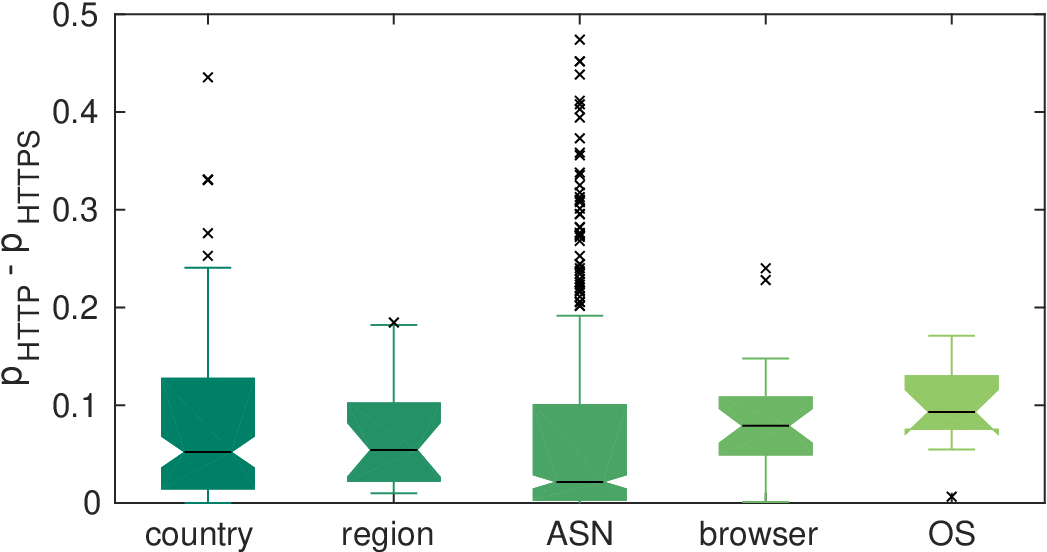
The more subtle question that this raises is, given such dependency, can we really assert that HTTPS is “harder” than HTTP? The goal of assessing this question is addressed by McNemar’s test. The table shows that we must also reject the null in this case, and hence we have significant evidence that the two measurements have different levels of difficulty. The direction can be seen from the differences in probabilities, e.g., see Table 3, and Figure 1.
This finding must be carefully qualified, noting here that although the two measurements are matched, they typically occur in order, and hence, there may be some effect on the second measurement resulting from the state created by the first. So we must understand that this experiment concerns lifting a connection up from HTTP to HTTPS, not an arbitrary HTTPS connection (see the detailed notes in Section 3).
| Success proportion | |||||
|---|---|---|---|---|---|
| OS ID | HTTP | HTTPS | Difference | ||
| 1 | 0.019 | 0.977 | 0.847 | 0.130 | |
| 2 | 0.077 | 0.983 | 0.917 | 0.066 | |
| 3 | 2.577 | 0.968 | 0.881 | 0.088 | |
| 4 | 0.655 | 0.978 | 0.903 | 0.075 | |
| 5 | 0.039 | 0.995 | 0.989 | 0.006 | |
| 6 | 7.337 | 0.969 | 0.881 | 0.088 | |
| 7 | 8.511 | 0.988 | 0.891 | 0.098 | |
| 8 | 0.036 | 0.978 | 0.873 | 0.105 | |
| 9 | 0.052 | 0.993 | 0.825 | 0.169 | |
| 10 | 0.647 | 0.981 | 0.881 | 0.100 | |
| 11 | 2.216 | 0.966 | 0.884 | 0.081 | |
| 12 | 0.155 | 0.974 | 0.820 | 0.154 | |
| 13 | 0.016 | 0.990 | 0.819 | 0.171 | |
| 14 | 10.566 | 0.963 | 0.909 | 0.055 | |
| Overall | 32.903 | 0.973 | 0.893 | 0.080 | |
As well, care must be taken that the results have not been created by some underlying covariate. As an initial window into this question, consider the boxplot [29, 30] shown in Figure 1. The plot shows (shaded) the interquartile range, and as a notch the confidence interval for the estimate of the median value, of the difference . If the covariates were truly irrelevant, we would expect that interquartiles and medians should be the same (within the ranges of natural variation shown by the confidence in intervals in the case of the median), and hence the chart provides evidence that the covariates are important.
Therefore we now consider what part the covariates (country, region, ASN, OS and browser) play. We chose, at least initially, to be conservative by only analyzing groupings with at least 500 measurements. It is quite possible that smaller groupings would have been amenable to analysis, but we had no need (here) to describe the relationships between all of the rarer groupings, as our goal was to ascertain whether the overall result was supported on a finer level of granularity.
The number 500 was chosen through an initial exploratory analysis, which noted that some of the probabilities in question were quite close to 1, and hence the typical statistical rules of thumb required a moderately large number of observations. As we did not know exactly what these probabilities were a priori, we chose a conservative lower bound. We also found, as Table 4 shows, that excluding the groups with a small number of observations excluded a small percentage of the data.
As noted above, we worked with anonymized data, e.g., region codes were remapped. We were not aiming here for strict anonymization of all details, but aimed to (i) prevent individual identification without extraordinary efforts, and (ii) ensure that the statistical analyses were not biased by preconceived notions about different Internet regions. Limiting the data to groups with at least 500 measurements also facilitated this blinding.
The results can be seen in Figure 2, which shows histograms of the distributions of -values over the set of tests grouped by the various categorical covariates described above. The important fact to note is that most of the -values are small. We cannot see (at the resolution of the plot) whether the -values fall below the threshold, so Table 4 summarizes the tests, and shows that, in a large proportion of the cases, we rejected the null-hypotheses. Thus we have significant evidence for these properties in many of the groupings, and as such, our model should incorporate these features.


Interestingly, ASN is the grouping with the lowest proportion of rejected null-hypotheses, while we might have expected that ASN would have a larger effect on the network aspects of the problem. However, remember the large Bonferroni correction in this case, which leads to a rather conservative test.
There is much more work to be done in this area. Multiple-comparisons could be applied, for instance, to differentiate regions or some other covariates, in order to understand which observed differences were significant, and which were “noise.” However, in doing so there would be comparisons for regions, and more importantly, we are then performing a set of hypothesis tests that are not all independent of each other, complicating the test procedure greatly. Moreover, much of this theory has been developed in domains where the conduct of each measurement requires a physical or social experiment, and therefore large sets of costly measurements. Instead, as our next step, we opt to apply an approach called Rasch modeling described below.
4.2 Rasch Modeling
The disadvantage of the previous tests is firstly that they provide only a yes/no answer (or really a yes/maybe answer), while we would like, for instance, to be able to say whether a particular country is falling behind in its ability to support HTTPS. Secondly, this approach breaks the data into blocks and analyzes each separately, but there are advantages in analyzing it in toto.
| covariate | % of data | Fisher | McNemar | |
|---|---|---|---|---|
| country | 119 | 99.6 | 0.580 | 0.840 |
| region | 20 | 100.0 | 0.800 | 0.950 |
| ASN | 458 | 93.1 | 0.277 | 0.555 |
| browser | 28 | 99.9 | 0.821 | 0.929 |
| OS | 14 | 100.0 | 0.929 | 1.000 |
There are many approaches that could be adopted to solve this problem. Here, we consider an approach broadly called Item Response Theory (IRT). This is an area best illustrated by its application to the analysis of examinations. In this context, an exam consists of a list of questions, performed by students. At its simplest, each student answers each question either correctly, or not, forming a set of binary response variables , where is the student (in our context an observation) and is the question (a measurement).
Within IRT, one of the oldest and most popular strategies is called Rasch modeling [31, 32]. This posits that there are latent variables, namely:
- 1.
the ability or proficiency of student , denoted ; and
- 2.
the difficulty of question , denoted
that determine the probability of a student answering question correctly. The variables are latent in that we do not know them a priori.
In its simplest case, i.e., a dichotomous response, we have response variables , which are Bernoulli random variables indicating a successful answer to a question, whose probabilities are modeled as
| (1) |
The probability function above is described as logistic, and has an inverse called the logit function. Taking the logit we get
| (2) |
Thus we have a simple linear relationship at this point.
Rasch modeling is one of the simplest, and yet most enduring approaches to IRT [31, 32], because it has a number of appealing properties:
- •
It simplifies the relationships so that reasonable estimates can be made, even though we have only one instance of each student attempting each question;
- •
Unlike the conventional statistical paradigm, where parameters are fit to data, and accepted or rejected based on the accuracy of the fit, in Rasch modeling the objective is to obtain “data” that fit the model, i.e., the latent predictor variables.
- •
The Rasch model embodies the principle of invariant comparison, in which (broadly speaking) the effect on the outcome of a question is separated into the affect of the respondent, and the question’s difficulty.
The model is not limited to modeling examinations, but can be applied to any set of observations such as we have. In the traditional dichotomous Rasch analysis, we analyze each student who answers questions correctly or incorrectly, but in our data, we have (i) a large number of observations, well above that normally considered in IRT, and (ii) we have no particular interest in the performance of individuals.
To be precise, we could consider each observation as one “student” participating in the measurements, and analyze them all separately, but this would be both banal (since performance at this level of granularity is immaterial) and needlessly computationally complex. In practice, we would like to group measurements into meaningful partitions (a partition is a collection of subsets that are disjoint and cover the original set).
However, when this is done, we depart from the pure simplicity of the basic Rasch model. There are at least two alternative approaches; we might think of these subsets as either being comprised of:
- 1.
a group of similar students, who have an underlying property in common (usually we assume members of the group have proficiencies that are random variables with a common mean and variance); or
- 2.
a group of repeated measurements of a “student” who corresponds to the particular subset, and the responses are now Binomial random variables corresponding to the number of correct measurements within the subset.
The two assumptions lead naturally to different solution algorithms.
The first model still follows (2), but now we assume that , where is the group mean proficiency, and is the standard deviation within the group, parameters which we need to estimate.
This approach is perhaps more advanced, in that exact results are known, and there are off-the-shelf solvers using Marginal Maximum Likelihood Estimation (MMLE). We use IRTm [33, 34], a Matlab toolbox allowing quite general models to be estimated. MMLE also has the disadvantage that we assume a model for the distribution of the grouped student proficiencies.
Moreover, in its model a categorical variable with categories is deconstructed into binary variables, each an indicator for one possible state of the original variable. This has the advantage of simplifying the model, but at the expense of greatly increasing the number of variables. For instance, in our filtered data, we have 119 countries, and so we must construct a covariate vector consisting of 119 binary elements. The result is that the estimation procedure takes more memory and time.
The results are illustrated below, in conjunction with those of the second approach.
The second approach takes a simpler model, that
| (3) |
for , where is the th group. We now only estimate a group proficiency , not individual proficiencies. This has the disadvantage that it might not be able to fit the data as accurately, but it does free us from distributional assumptions.
However, the standard Binomial Rasch models for repeated measurements assume each measurement is repeated a fixed number of times. For instance, in partial-credit Rasch models [35], a student may obtain some proportion of the marks for a question, but each student answers the same question, with the same total possible marks. But in our groupings, the number of “total marks” would vary, depending on the number of observations that fall into the group. This case does not appear to have been treated in the literature, and hence we wrote our own Alternating Least Squares (ALS) algorithm (also in Matlab) to estimate the parameters.
The algorithm alternates between fitting the and the values, keeping the alternative parameters fixed. It also needs an additional fixed point of reference (because the variables and are not otherwise uniquely determined), which we fix without loss of generality, to be .
Ideally, we could group by all covariates at once. However, this results in few measurements per group, and a very large number of covariates in the MMLE approach, while in the ALS approach, we end up with few observations in many of the bins, due to the combinatorial nature of the number of bins. Thus we leave a combined covariate analysis until later, and analyze each of the categories as separate groupings, as we did in the statistical tests above. As before, we again made the highly conservative choice to consider only groupings with at least 500 measurements, which is also helpful in refining the number of categories for variables, and hence reducing the computation load for MMLE.
We assessed the two approaches in this (somewhat non-standard) application by comparing computation times, and Root-Mean-Square (RMS) errors, as shown in Figure 3. All computations were made on an 8 core, Intel i7-6900K 3.2 GHz, running Linux Mint 18, and Matlab R1016b. Note that the largest case for the MMLE algorithm did not complete (within 24 hours), The ALS algorithm was orders of magnitude more accurate and faster. So in what follows we focus on the ALS approach. Note also that the estimation errors in ALS reach a maximum in the order of 5%, which is reasonable given the problem of interest, but it works better on the cases with a smaller number of variates, and so we ignore ASN for the moment.


The first detail to consider is the values, indicating the difficulty in completing the two measurements (HTTP, and HTTPS). The estimated values are shown in Table 5, along with their difference, which is an indication of the additional difficulty of the HTTPS measurement. From all points of view, HTTPS is more difficult than HTTP. The country/region and the browser/OS covariate groupings also show some consistency, indicating that these variables act on the measurements in somewhat the same way, which is not surprising.
| country | region | browser | OS | |
|---|---|---|---|---|
| -5.26 | -4.91 | -3.94 | -3.99 | |
| -2.92 | -2.74 | -2.29 | -2.12 | |
| Difference | 2.34 | 2.16 | 1.65 | 1.86 |
The second set of parameters to examine are the values, namely, the ability or proficiency of a particular covariate group to perform the measurement, large values being better. Figure 4 shows the distribution of values for the region, OS, and browser covariates. We see that they might be coarsely considered to follow a Normal distribution. The data by OS fit this assumption least well, but remember that there are only 14 values here, so we do not expect to see a clean fit. We expect to see some natural variation here, because of estimation error, and measurement noise. The excluded case, the data by ASN, present a much wider range of variation than the cases shown, and we hypothesize that this variability is real, and important, but defer finalizing this conclusion.

We also see outliers, here defined as those values that fall more than 1.96 times the standard deviation from the mean, i.e., outside the 95th percentiles. These are not extreme outliers, but these cases certainly warrant further investigation. There are outliers on the positive side: five countries, one browser, and one OS, each of which found the measurements easier to correctly perform. These are of no particular concern, though it might be interesting to investigate them further, to understand if their success could be duplicated. On the downside, there is only one outlier country.
There are two main conclusions to be drawn.
- 1.
The measurements show that there is significantly more difficulty in performing HTTPS than HTTP measurements. The difference is often small, necessitating some extra care in order to determine whether the difference is significant.
- 2.
There are country, OS, and browser differences, mainly important through a small set that exhibits more extreme variations from the norm.
Regarding the latter conclusion, we have deliberately kept the blinding in our analysis here. Even though it is not necessary, and for operational tasks such as improving the current situation, an organization could use the same analysis to focus efforts on improvements. It is not within the ambit of this paper to make statements for or against particular regions, browsers or OSes.
This analysis has one major limitation — we considered the different groupings separately, instead of together. Moreover, we wish to perform our investigations of outliers in more detail (particularly for ASN), and explore how components interact, e.g., in the above analysis we tended to highlight countries that performed badly in both tests, not just HTTPS.
4.3 Generalized Linear Mixed Models
The above approach is appealing in its simplicity, but deeper analysis is possible. For instance, analysis of ASN proved problematic in the above tests and analysis, at least in part because there are many more ASNs than any of the other categories. Another statistical tool is a Generalized Linear Model (GLM) [36]. This is a natural generalization of linear modeling to cope with non-Gaussian random variables (in our case, we have Bernoulli (0/1) random variables).
This has the potential to be applied to a wide variety of analyses, but it requires refinement to the specifics of the problem of interest, and we must also be able to perform the computations, which will be more challenging than those of the previous tests.
In some ways, the idea of a GLM is similar to that of Rasch. We model the probability of success via an inverse link function to a linear combination of predictors. For Bernoulli data, we would (as in the Rasch model) use the logit link function. However, there is a subtle difference in the sense that in Rasch modeling, we think of each student having a probability of success. Instead, we now think of a generic Bernoulli response variable , for which we have observations, but now the probability of success is a function of some set of predictors, i.e.,
| (4) |
where is the response we are interested in — here it will be , and the are parameters to be estimated, linking the outcome to the predictor as a so-called fixed effect.
The predictors could include the covariates already discussed (country, region, ASN, browser and OS), but note that as in the MMLE Rasch analysis, categorical predictors such as region, with possible values, must be converted into a binary vector of length , indicating which category applies. This leads us to the problem of estimating a potentially large number of parameters . The predictors could also include our previous test result .
At least initially, the particular effect of each country is not material. Our initial concern is to remove confounding effects of the country from the analysis, so that the questions of interest can be answered. If this is the case, we can instead include a covariate as a random effect, leading to the idea of a Generalized Linear Mixed Model (GLMM), incorporating a mixture of fixed and random effects. In this formulation, we might take random intercepts and then
| (5) |
where we now estimate different probabilities for each country , with a random-effect (which is a change to the intercept). We could add similar random effects for the other covariates. The key difference here between the fixed-effect parameters and the random-effects parameters are that we assume little about the fixed-effect parameters, whereas the are assumed to come from a Normal distribution, i.e., , whose variance is a parameter to be estimated here. This assumption allows for estimation despite the potentially large number of values , because the model needs only the overall variance estimate, not the individual parameters. Or, to be more clear, if we were to make predictions from this model, we would not retain the individual values, but only the variance .
Random effects are used particularly when we have a predictor or covariate that is not repeatable. For instance, in examinations, we would not test students using the same questions twice. Here, the countries observed are formed through the sampling process, and so the number of observations per country is not set by the experimenters. We cannot repeat exactly the same experiment at that level, so it is reasonable to include these covariates as random effects. However, we might want to change that decision if we were asking a particular question about the impact of a particular country on the results, when it would be appropriate to include a predictor for that particular country as a fixed effect. For instance, we could ask the question “Is country X being left behind, taking into account the effects of all of the other covariates?” Including the other covariates as random effects avoids the problem that we might believe country X is being left behind, even though the result arises because country X has a preponderance of users on OS Y, which is the real cause.
Another advantage of random effects is that they lead to relatively more efficient algorithms for estimation, because we only have to estimate one parameter instead of one per category. Here, we focus on the analysis using as the only fixed effect, and consider which covariates are important to include in any model. That is, we use the analysis technique to explore whether we should incorporate region, for instance, into our model.
There is a close connection between Rasch models and GLMM [37]. In fact, the GLMM might be thought of as a type of generalized Rasch model where the groupings considered above are all potentially considered at once as random effects.
Here we perform a Maximum Likelihood Estimation (MLE) of the parameters of these models using R [38], and the lme4 [39] package.
We do not consider arbitrary problems combining all factors at once, due to the long computational times required for these cases. Moreover, some factors are “nested” inside others, e.g., countries in regions, and to a lesser extent, browsers in OS. This creates additional complexity in modeling this structure in the regression. We will start by considering the simple problems, including one covariate as a random effect at a time.
Note also that in this section of the analysis, computational requirements limit us to considering an sub-sample of our data. The algorithms involved are very much more computationally complex, so for the moment we sub-sample 10% (randomly without replacement) of our original set. However, we no longer restrict our attention to groupings with over 500 observations.
The particular model we consider first is
| (6) |
where observation , i.e., the observation falls into group of a particular covariate, included through a random intercept , and the fixed effect is the influence that the 1st measurement has on the 2nd (the result). Here captures the marginal increase in the chance of success in the second measurement, given the first.
Apart from considering the question of quantitatively inferring the effect of the first measurement on the second (we already know from our Fisher test that there is typically some effect, but not how much), we will also use this approach to assess which covariates are necessary in our modeling enterprise. We will do so using Information Criteria (IC), specifically Akaike IC (AIC) [40] and Bayesian IC (BIC) [41].
These criteria allow one to determine an appropriate trade-off between the accuracy usually obtained by including additional parameters into a model, against the costs of addition parameters, particular in the reduction of generality of the model, i.e., the dangers of over-fitting. In general, models with a lower IC are preferred, though there is no single perfect IC [42], and so two are used here to confirm conclusions.
We adopt a greedy approach to inclusion of covariates: we start by considering the benefit of including a single covariate, and we choose the one that decreases the IC by the largest amount. We then consider the benefit of including a second covariate and so on. An advantage this grants is that we can update an existing model, adding in extra covariates instead of starting from scratch, saving additional computation time.
| Covariates | AIC | BIC | time (s) |
|---|---|---|---|
| - | 212244.1 | 212265.5 | 0.7 |
| C | 202988.5 | 203020.5 | 34.0 |
| R | 206266.5 | 206298.5 | 26.5 |
| A | 191988.6 | 192020.7 | 90.1 |
| B | 210905.8 | 210937.8 | 28.5 |
| O | 211560.8 | 211592.9 | 28.7 |
| A,C | 191657.5 | 191700.2 | 153.0 |
| A,R | 191986.5 | 192029.2 | 253.5 |
| A,B | 190974.9 | 191017.6 | 166.1 |
| A,O | 191424.6 | 191467.3 | 174.7 |
| A,B,C | 190554.3 | 190607.7 | 493.2 |
| A,B,R | 190922.2 | 190975.6 | 246.4 |
| A,B,O | 190729.5 | 190782.9 | 304.2 |
| A,B,C,R | 190553.5 | 190617.5 | 384.9 |
| A,B,C,O | 190187.1 | 190251.2 | 397.3 |
| A,B,C,O,R | 190178.3 | 190253.0 | 574.9 |
Table 6shows the process, where we have first computed the GLM with only the fixed effect, then updated this model to include one other covariate. Of the possibilities, ASN realises the largest reduction in both ICs, and so we add this into our model.
We then update by adding a second covariate, the winning case being browser, i.e., the case listed as model (A,B). In the following steps the winners are country and OS. Note that the selected covariates (see boldface entries) present a decreasing sequence of ICs.
However, when we consider including region, we see that the IC do not both decrease (specifically BIC indicated in red increases), and hence we will not add this addition covariate. This is slightly conservative, but the marginal improvement is at best very small.
The conclusion is that the alternative covariates add little additional information. This is somewhat obvious: once we know the country, we know the region. However, the process above (i) confirms that all of the other covariates should be included, and (ii) confirms that we prefer country over region as a explanatory covariate.
Once we have a model, we can examine it in detail. For the final model (A,B,C,O), we rerun the estimation procedure for the full dataset. The total analysis took 1.5 hours. Table 7 shows the results.
The small -values for the fixed effects indicate a high degree of significance. As we expect, the result of the first measurement is related to that of the second. The positive value of indicates that success in the first measurement improves our chance in the second.
The values show the variance of the random effect parameters for each type of covariate. As might be expected, they are decreasing because the are listed in order of importance as measured by the IC.
Also noteworthy is the scale of the effects. The give a measure of the variability of the random effect associated with the covariate. It could be considered against the scale of , which tells the marginal increase resulting from success in the first measurement. We can see that the variability of effects due to ASN are of a similar magnitude to , and the affect due to country is not far behind. Effects due to browser and OS are somewhat smaller.
| Parameter | value | std. error | -value |
|---|---|---|---|
| 2.7960 | 0.0214 | ||
| 1.7236 | 0.0068 | ||
| 2.0971 | - | - | |
| 1.3177 | - | - | |
| 0.7944 | - | - | |
| 0.4181 | - | - |
In any statistical analysis, care must be exercised when asserting causality. Just because two events are correlated, we cannot assert causality. However, the GLMM presented has the advantage that it can provide predictions. That is, we could use this model to predict the outcome of our experiment in the future, based on the various covariates, and hence provide some insights through this means.
One last important insight is that the dependence on the covariates indicates that the results are not an artefact of APNIC’s measurement infrastructure, as that would remove dependency on point of origin effects.
GLMMs have great capabilities, and we have only scratched the surface here. We could consider cross-variable effects, hierarchical models, and so on, and use this to build more focused experiments to understand, for instance, the details of how some HTTPS connections fail, in order to improve the situation.
5 Conclusion and Further Work
Using a large set of measurements, and detailed statistical modeling we have shown that a small cohort of users in the real world will be adversely affected if HTTPS is adopted universally. That cohort is not a large proportion of Internet users, but those users deserve our attention: What are we going to do, to provide them with a secure network?
We have categorized measurements by country and region, their provider (origin ASN), browser and operating system, and shown that all of these factors affect a client’s facility with HTTPS. The range of factors points to a range of causes for the blockages. The browser/OS combination suggests a technological problem, but the other covariates suggest problems based in the network near the clients.
In the future, we plan to further investigate, and use the details of the analysis to help focus efforts onto relevant development to mitigate the problem. We also aim to repeat this study to consider the rate of change in this cohort of users, to understand if this problem is growing, or shrinking over time.
The use of careful statistical methods was vital in this study. The underlying signal is weak, and hence required “amplification” and careful analysis so as to be able to make confident statements.
Acknowledgements
We would like to thank the Australian Research Council for funding through the Centre of Excellence for Mathematical & Statistical Frontiers (ACEMS), and grant DP110103505.
The Javascript code used by APNIC originates in a library written by Emile Aben, RIPE-NCC.
APNIC Labs has received support and in-kind assistance from Google, ICANN, RIPE-NCC and ISC in conducting its web experiments.
References
- [1] “HTTPS everywhere,” on-line: downloaded April 24th, 2017, https://www.eff.org/https-everywhere.
- [2] “HTTPS everywhere,” Google I/O, https://docs.google.com/presentation/d/15H8Sj-Zol1tcum0CSylhmXns5r7cvNFtzYrcwAzkTjM/edit#slide=id.g12f3ee71d_10.
- [3] “HTTPS as a ranking signal,” https://webmasters.googleblog.com/2014/08/https-as-ranking-signal.html, August 2016.
- [4] “The HTTPS-Only standard,” on-line: downloaded April 24th, 2017, https://https.cio.gov/.
- [5] A. Goldberg, R. Buff, and A. Schmitt, “A comparison of HTTP and HTTPS performance,” in CMG98, 1998, http://www.cs.nyu.edu/artg/research/comparison/comparison.html.
- [6] C. Coarfa, P. Druschel, and D. S. Wallach, “Performance analysis of tls web servers,” ACM Trans. Comput. Syst., vol. 24, no. 1, pp. 39–69, Feb. 2006. [Online]. Available: http://doi.acm.org/10.1145/1124153.1124155
- [7] D. Naylor, A. Finamore, I. Leontiadis, Y. Grunenberger, M. Mellia, M. Munafò, K. Papagiannaki, and P. Steenkiste, “The cost of the ”S” in HTTPS,” in 10th ACM International on Conference on Emerging Networking Experiments and Technologies (CoNEXT), New York, NY, USA, 2014, pp. 133–140. [Online]. Available: http://doi.acm.org/10.1145/2674005.2674991
- [8] D. Beaver, “HTTP2 expression of interest,” on-line: downloaded April 24th, 2017, July 2012, http://lists.w3.org/Archives/Public/ietf-http-wg/2012JulSep/0251.html.
- [9] “HTTPS usage statistics on top websites,” on-line: downloaded April 24th, 2017, https://statoperator.com/research/https-usage-statistics-on-top-websites/.
- [10] “HTTPS usage,” on-line: downloaded April 24th, 2017, https://www.google.com/transparencyreport/https/metrics/?hl=en.
- [11] G. Michaelson and G. Huston, “Experience with large-scale end user measurement techniques,” in Telecommunication Networks and Applications Conference (ATNAC), 2014 Australasian. IEEE, 2014, pp. 1–5.
- [12] M. Casado and M. J. Freedman, “Peering through the shroud: The effect of edge opacity on IP-based client identification,” in Proceedings of the 4th USENIX Conference on Networked Systems Design & Implementation, ser. NSDI’07, 2007, pp. 13–13. [Online]. Available: http://dl.acm.org/citation.cfm?id=1973430.1973443
- [13] S. Burnett and N. Feamster, “Encore: Lightweight measurement of web censorship with cross-origin requests,” in ACM SIGCOMM, 2015, pp. 653–667. [Online]. Available: http://doi.acm.org/10.1145/2785956.2787485
- [14] Z. Durumeric, J. Kasten, M. Bailey, and J. A. Halderman, “Analysis of the HTTPS certificate ecosystem,” in ACM Sigcomm Internet Measurement Conference, 2013, pp. 291–304. [Online]. Available: http://doi.acm.org/10.1145/2504730.2504755
- [15] B. Laurie and C. Doctorow, “Secure the internet,” Nature, vol. 491, pp. 325–6, 2012.
- [16] F. Callegati, W. Cerroni, and M. Ramilli, “Man-in-the-middle attack to the HTTPS protocol,” IEEE Security Privacy, vol. 7, no. 1, pp. 78–81, Jan 2009.
- [17] D. Ranathunga, M. Roughan, H. Nguyen, P. Kernick, and N. Falkner, “Case studies of scada firewall configurations and the implications for best practices,” IEEE Transactions on Network and Service Management, 2016, http://ieeexplore.ieee.org/stamp/stamp.jsp?tp=&arnumber=7529047&isnumber=5699970.
- [18] A. Wool, “A quantitative study of firewall configuration errors,” Computer, IEEE, vol. 37, no. 6, pp. 62–67, 2004.
- [19] “SSL/TLS - typical problems and how to debug them,” on-line: downloaded April 24th, 2017, https://maulwuff.de/research/ssl-debugging.html.
- [20] J. P. Shaffer, “Multiple hypothesis testing,” Annu.Rev.Psychol., vol. 46, pp. 561–584, 1995.
- [21] P. H. Westfall, J. F. Troendle, and G. Pennello, “Multiple McNemar tests,” Biometrics, vol. 66, no. 4, pp. 1185–1191, 1995.
- [22] A. Agresti, Categorical Data Analysis, 2nd ed. Wiley, 2002.
- [23] “ngx_txid,” https://github.com/APNIC-Labs/ngx_txid, accessed May 16th, 2017.
- [24] “nginx,” http://nginx.org/, accessed May 16th, 2017.
- [25] “Standard country or area codes for statistical use (M49),” https://unstats.un.org/unsd/methodology/m49/, accessed May 16th, 2017.
- [26] A. H. Rasti, N. Magharei, R. Rejaie, and W. Willinger, “Eyeball ASes: From geography to connectivity,” in ACM Sigcomm IMC, Melbourne, Australia, 2010.
- [27] “GeoIP databases & services: Industry leading IP intelligence,” https://www.maxmind.com/en/geoip2-services-and-databases, accessed May 16th, 2017.
- [28] “A Python implementation of the UA parser,” https://github.com/ua-parser/uap-python, accessed May 16th, 2017.
- [29] R. McGill, J. W. Tukey, and W. A. Larsen, “Variations of box plots,” The American Statistician, vol. 32, no. 1, pp. 12–16, 1978. [Online]. Available: http://www.jstor.org/stable/2683468
- [30] H. Wickham and L. Stryjewski, “40 years of boxplots,” had.co.nz, Tech. Rep., 2012, http://vita.had.co.nz/papers/boxplots.html.
- [31] B. Wright and M. Mok, Introduction to Rasch Measurement: Theory, Models, and Applications. Journal of Applied Measurement, 2004, ch. An Overview of the Family of Rasch Measurement Models, jampress.org/irmch1.pdf.
- [32] B. D. Wright, “Solving measurement problems with the Rasch model,” Journal of Educational Measurement, vol. 14, no. 2, pp. 97–116, 1977. [Online]. Available: http://www.jstor.org/stable/1434010
- [33] J. Braeken and F. Tuerlinckx, “Investigating latent constructs with item response models: a MATLAB IRTm toolbox,” Behavior Research Methods, vol. 414, no. 4, pp. 1127–37, 2009.
- [34] “IRTm,” https://ppw.kuleuven.be/okp/software/irtm/.
- [35] G. M. Masters, “A rasch model for partial credit scoring,” Psychometrika, vol. 47, no. 2, pp. 149–174, 1982.
- [36] P. McCullagh and J. A. Nelder, Generalized Linear Models, 2nd ed. Chapman & Hall, 1989.
- [37] H. Doran, D. Bates, P. Bliese, and M. Dowling, “Estimating the multilevel rasch model: With the lme4 package,” Journal of Statistical Software, vol. 20, no. 2, 2007.
- [38] R Core Team, R: A Language and Environment for Statistical Computing, R Foundation for Statistical Computing, Vienna, Austria, 2013. [Online]. Available: http://www.R-project.org/
- [39] D. Bates, M. Mächler, B. Bolker, and S. Walker, “Fitting linear mixed-effects models using lme4,” Journal of Statistical Software, vol. 67, no. 1, pp. 1–48, 2015.
- [40] H. Akaike, “A new look at statistical model identification,” IEEE Trans. Autom. Control, vol. 19, no. 6, pp. 716–723, Dec. 1974.
- [41] G. E. Schwarz, “Estimating the dimension of a model,” Annals of Statistics, vol. 6, no. 2, pp. 461–464, 1978.
- [42] P. Tune, K. Cho, and M. Roughan, “A comparison of information criteria for traffic model selection,” in 10th International Conference on Signal Processing and Communications Systems (ICSPCS), Gold Coast, Australia, December 2016.