Emerging Translational Variance: Vacuum Polarization Energy of the $\mathbf{\phi^{6}}$ Kink

It is of general interest to compute quantum corrections to classical field configurations like soliton solutions that are frequently interpreted as particles. On top of the wish list we find the energies that predict particle masses. The quantum correction to the energy can be quite significant because the classical field acts as a background that strongly polarizes the spectrum of the quantum fluctuations about it. For that reason the quantum correction to the classical energy is called vacuum polarization energy (VPE). Here we will consider the leading, i.e. one loop, contribution.

Field theories that have classical soliton solutions in various topological sectors deserve particular interest. Solitons from different sectors have unequal winding numbers and the fluctuation spectrum changes significantly from one sector to the other. For example, the number of zero modes is linked to the number of (normalizable) zero modes that in turn arise from the symmetries that are spontaneously broken by the soliton. Of course, the pattern of spontaneous symmetry breaking is subject to the topological structure. On the other hand, the winding number is typically identified with the particle number. The prime example is the Skyrme model[1, 2] wherein the winding number determines the baryon number[3, 4]. Many properties of baryons have been studied in this soliton model and its generalization in the past[5]. More recently configurations with very large winding numbers have been investigated[6] and these solutions were identified with nuclei. To obtain a sensible understanding of the predicted nuclear binding energies it is, of course, important to consider the VPE, in particular when it is expected to strongly depend in the particle number. So far this has not been attempted for the simple reason that the model is not renormalizable. A rough estimate[8]¹¹ 1 See Ref.[7] for a general discussion of the Skyrmion’s quantum corrections and further references on the topic. in the context of the H–dibaryon[9, 10] suggests that the VPE strongly reduces the binding energy of multi–baryon states.

As already mentioned, one issue for the calculation of the VPE is renormalization. Another important one is, as will be discussed below, that the VPE is (numerically) extracted from the scattering data for the quantum fluctuations about the classical configuration[11]. Though this so–called spectral method allows for a direct implementation of standard renormalization conditions it has limitations as it requires sufficient symmetry for a partial wave decomposition. This may not be possible for configurations with an intricate topological structure associated with large winding numbers.

The $\phi^{6}$ model in $D=1+1$ dimensions has soliton solutions with different topological structures[12, 13] and the fluctuations do not decouple into a parity channels. The approach employed here is also based on scattering data but advances the spectral method such that no parity decomposition is required. We will also see that it is significantly more effective than previous computations[14, 15, 16] for the VPE of solitons in $D=1+1$ dimensions that are based on heat kernel expansions combined with $\zeta$–function regularization techniques[17, 18, 19].

Although the $\phi^{6}$ model is not fully renormalizable, at one loop order the ultra--violet divergences can be removed unambiguously. However, another very interesting phenomenon emerges. The distinct topological structures induce non--equivalent vacua that manifest themselves via different dispersion relations for the quantum fluctuations at positive and negative spatial infinity. At some intermediate position the soliton mediates between these vacua. Since this position cannot be uniquely determined the resulting VPE exhibits a translational variance. This is surprising since, after all, the model is defined through a local and translational invariant Lagrangian. In this paper we will describe the emergence of this variance and link it to the different level densities that arise from the dispersion relations. To open these results for discussion²² 2 The present paper reflects the author’s invited presentation at the $5^{\rm th}$ Winter Workshop on Non-Perturbative Quantum Field Theory based on the methods derived in Ref.[20] making some overlap unavoidable. it is necessary to review in detail the methods developed in Ref.[20] to compute the VPE for backgrounds in one space dimension that are not (manifestly) invariant under spatial reflection.

Following this introductory motivation we will describe the $\phi^{6}$ model and its kink solutions. In chapter III we will review the spectral method that ultimately leads to a variant of the Krein–Friedel–Lloyd formula[21] for the VPE. The novel approach to obtain the relevant scattering data will be discussed in chapter IV and combined with the one–loop renormalization in chapter V. A comparison with known (exact) results will be given in chapter VI while chapter VII contains the predicted VPE for the solitons of the $\phi^{6}$ model. Translational variance of the VPE that emerges from the existence of non–equivalent vacua will be analyzed in chapter VIII. We conclude with a short summary in chapter IX.

In $D=1+1$ dimensions the dynamics for the quantum field $\phi$ are governed solely by a field potential $U(\phi)$ that is added to the kinetic term

$$\mathcal{L}=\frac{1}{2}\partial_{\mu}\phi\partial^{\mu}\phi-U(\phi)\,.$$

(1)

For the $\phi^{6}$ model we scale all coordinates, fields and coupling constants such that the potential contains only a single dimensionless parameter $a$

$$U(\phi)=\frac{1}{2}\left(\phi^{2}+a^{2}\right)\left(\phi^{2}-1\right)^{2}\,.$$

(2)

In either case the classical mass is $E_{\rm cl}={\textstyle\frac{1}{4}}={\textstyle\frac{1}{2}}\lim_{a\to 0}E_{\rm cl}(a)$. This relation for the classical energies reflects the fact that as $a\to 0$ the solution $\phi_{K}(x)$ disintegrates into two widely separated structures one corresponding to $\phi_{K_{1}}(x)$ the other to $\phi_{K_{2}}(x)$.

The computation of the VPE requires the construction of scattering solutions for fluctuations about the soliton. In the harmonic approximation the fluctuations experience the potential

$$V(x)=\frac{1}{2}\frac{\partial^{2}U(\phi)}{\partial\phi^{2}}\Big|_{\phi=\phi_{\rm sol}(x)}$$

(6)

generated by the soliton ($\phi_{\rm sol}=\phi_{K}$, $\phi_{K_{1}}$ or $\phi_{K_{2}}$).

These three potentials are shown in figure 3. For $a\neq 0$ the potential is invariant under $x\leftrightarrow-x$. But the particular case $a\equiv 0$ is not reflection symmetric, though $x\leftrightarrow-x$ swaps the potentials generated by $\phi_{K_{1}}$ and $\phi_{K_{2}}$. The loss of this invariance disables the separation of the fluctuation modes into symmetric and anti–symmetric channels, which is the one dimensional version of partial wave decomposition. Even more strikingly, the different topological structures in the $a=0$ case cause $\lim_{x\to-\infty}V(x)\neq\lim_{x\to\infty}V(x)$, which implies different masses (dispersion relations) for the fluctuations at positive and negative spatial infinity.

The formula for the VPE, Eq. (12) below, can be derived from first principles in quantum field theory by integrating the vacuum matrix element of the energy density operator[22]. It is, however, also illuminative to count the energy levels when summing the changes of the zero point energies. This sum is $\mathcal{O}(\hbar)$ and thus one loop order ($\hbar=1$ for the units used here). We call the single particle energies of fluctuations in the soliton type background $\omega_{n}$ while the $\omega_{n}^{(0)}$ are those for the trivial background. Then the VPE formally reads

$$E_{\rm vac}=\frac{1}{2}\sum_{n}\left(\omega_{n}-\omega_{n}^{(0)}\right)\Bigg|_{\rm ren.}=\frac{1}{2}\sum_{j}\epsilon_{j}+\frac{1}{2}\int_{0}^{\infty}dk\,\omega_{k}\,\Delta\,\rho_{\rm ren.}(k)\,,$$

(7)

where the subscript indicates that renormalization is required to obtain a finite and meaningful result. On the right hand side we have separated the explicit bound state (sum of energies $\epsilon_{j}$) and continuum (integral over momentum $k$) contributions. The latter involves $\Delta\,\rho_{\rm ren.}(k)$ which is the (renormalized) change of the level density induced by the soliton background. Let $L$ be a large distance away from the localized soliton background. For $x\sim L$ the stationary wave–function of the quantum fluctuation is a phase shifted plane wave $\psi(x)\sim{\rm sin}\left[kx+\delta(k)\right]$, where $\delta(k)$ is the phase shift (of a particular partial wave) that is obtained from scattering off the potential, Eq. (6). The continuum levels are counted from the boundary condition $\psi(L)=0$ and subsequently taking the limit $L\to\infty$. The number $n(k)$ of levels with momentum less or equal to $k$ is then extracted from $kL+\delta(k)=n(k)\pi$. The corresponding number in the absence of the soliton is $n^{(0)}(k)=kL/\pi$, trivially. From these the change of the level density is computed via

$$\Delta\,\rho(k)=\lim_{L\to\infty}\frac{d}{dk}\left[n(k)-n^{(0)}(k)\right]=\frac{1}{\pi}\frac{d\delta(k)}{dk}\,,$$

(8)

which is often referred to as the Krein–Friedel–Lloyd formula[21]. Note that $\Delta\,\rho(k)$ is a finite quantity; but ultra–violet divergences appear in the momentum integral in Eq. (7) and originate from the large $k$ behavior of the phase shift. This behavior is governed by the Born series

$$\delta(k)=\delta^{(1)}(k)+\delta^{(2)}(k)+\ldots$$

(9)

where the superscript reflects the power at which the potential, Eq. (6) contributes. Though this series does not converge³³ 3 For example, in three space dimensions the series yields $\delta(0)\to 0$ which contradicts Levinson’s theorem. for all $k$, it describes the large $k$ behavior well since $\delta^{(N+1)}(k)/\delta^{(N)}(k)\propto 1/k^{2}$ when $k\to\infty$. Hence replacing

$$\Delta\,\rho(k)\to\left[\Delta\,\rho(k)\right]_{N}=\frac{1}{\pi}\frac{d}{dk}\left[\delta(k)-\delta^{(1)}(k)-\delta^{(2)}(k)-\ldots-\delta^{(N)}(k)\right]$$

(10)

produces a finite integral in Eq. (7) when $N$ is taken sufficiently large. We have to add back the subtractions that come with this replacement. Here the spectral methods take advantage of the fact that each term in the subtraction is uniquely related to a power of the background potential and that Feynman diagrams represent an alternative expansion scheme for the vacuum polarization energy

$$\mbox{\parbox[l]{62.59596pt}{\vskip-54.06006pt$E_{\rm FD}^{N}[V]=$}}\psfig{file={fdseries.eps},height=54.06006pt,width=227.62204pt}\,.$$

(11)

The full lines are the free propagators of the quantum fluctuations and the dashed lines denote insertions of the background potential, Eq. (6), eventually after Fourier transformation. These Feynman diagrams are regularized with standard techniques, most commonly in dimensional regularization. They can thus be straightforwardly combined with the counterterm contribution, $E_{\rm CT}[V]$ with coefficients fully determined in the perturbative sector of the theory. This combination remains finite when the regulator is removed.

The generalization to multiple channels is straightforward by finding an eventually momentum dependent diagonalization of the scattering matrix $S(k)$ and summing the so--obtained eigenphase shifts. This replaces⁴⁴ 4 The proper Riemann sheet of the the logarithm is identified by constructing a smooth function that vanishes as $k\to\infty$. $\delta(k)\,\longrightarrow\,(1/2{\rm i}){\rm ln}{\rm det}\,S(k)$ and analogously for the Born expansions, Eqs. (9) and (10). Since after Born subtraction the integral converges, we integrate by parts to avoid numerical differentiation and to stress that the VPE is measured with respect to the translationally invariant vacuum. We then find the renormalized VPE to be, with the sum over partial waves re–inserted,

$$E_{\rm vac}[V]=\sum_{\ell}D_{\ell}\left\{\frac{1}{2}\sum_{j}\left(\epsilon_{\ell j}-m\right)-\int_{0}^{\infty}\frac{dk}{4\pi{\rm i}}\frac{k}{\sqrt{k^{2}+m^{2}}}\,\left[{\rm ln}\,{\rm det}\,S(k)\right]_{N}\right\}+E_{\rm FD}^{N}[V]+E_{\rm CT}[V]\,.$$

(12)

Here $D_{\ell}$ is the degree of degeneracy, e.g. $D_{\ell}=2\ell+1$ in three space dimensions. The subscript $N$ refers to the subtraction of $N$ terms of the Born expansion, as e.g. in Eq. (10). We stress that, with $N$ taken sufficiently large, both the expression in curly brackets and the sum $E_{\rm FD}^{N}[V]+E_{\rm CT}[V]$ are individually ultra–violet finite and no cut–off parameter is needed[23].

In this section we obtain the scattering matrix for general one dimensional problems and develop an efficient method for its numerical evaluation. This will be at the center of the novel approach to compute the VPE.

We first review the standard approach that is applicable when $V(-x)=V(x)$, e.g. left panel of figure 3. Then the partial wave decomposition separates symmetric $\psi_{S}(-x)=\psi_{S}(x)$ and anti–symmetric, $\psi_{A}(-x)=-\psi_{A}(x)$ channels. The respective phase shifts can be straightforwardly obtained in a variant of the variable phase approach[24] by parameterizing $\psi(x)={\rm e}^{{\rm i}[kx+\beta(k,x)]}$ and imposing the obvious boundary conditions $\psi^{\prime}_{S}(0)=0$ and $\psi_{A}(0)=0$. (The prime denotes the derivative with respect to $x$.) The wave–equation turns into a non–linear differential equation for the phase function $\beta(k,x)$. When solved subject to $\lim_{x\to\infty}\beta(k,x)=0$ and $\lim_{x\to\infty}\beta^{\prime}(k,x)=0$ the scattering matrix given by[11]

$$\frac{1}{2{\rm i}}\,{\rm ln}\,{\rm det}\,S(k)=-2{\sf Re}[\beta(k,0)]-{\rm arctan}\frac{{\sf Im}[\beta^{\prime}(k,0)]}{k+{\sf Re}[\beta^{\prime}(k,0)]}\,.$$

(13)

Linearizing and iterating the differential equation for $\beta(k,x)$ yields the Born series, Eq. (9). At this point it is advantageous to use the fact that scattering data can be continued to the upper half complex momentum plane[25]. That is, when writing $k={\rm i}t$, the Jost function, whose phase is the scattering phase shift when $k$ is real, is analytic for ${\sf Re}[t]\geq 0$. Furthermore the Jost function has simple zeros at imaginary $k={\rm i}\kappa_{j}$ representing the bound states. Formulating the momentum integral from Eq. (12) as a contour integral automatically collects the bound state contribution and we obtain a formula as simple as[22, 11]

$$E^{\rm(S)}_{\rm vac}=\int_{m}^{\infty}\frac{dt}{2\pi}\,\frac{t}{\sqrt{t^{2}-m^{2}}}\,\left[{\rm ln}\left\{g(t,0)\left(g(t,0)-\frac{1}{t}g^{\prime}(t,0)\right)\right\}\right]_{N}+E_{\rm FD}^{N}[V]+E_{\rm CT}[V]$$

(14)

for the VPE. Here $g(t,x)$ is the non–trivial factor of the Jost solution whose $x\to 0$ properties determine the Jost function. The factor function solves the differential equation

$$g^{\prime\prime}(t,x)=2tg^{\prime}(t,x)+V(x)g(t,x)\,,$$

(15)

with the boundary conditions $g(t,\infty)=1$ and $g^{\prime}(t,\infty)=0$; iterating $g(t,x)=1+g^{(1)}(t,x)+g^{(2)}(t,x)+\ldots$ produces the Born series.

In general, however, the potential $V(x)$ is not reflection invariant and no partial wave decomposition is applicable. Even more, there may exist different masses for the quantum fluctuations

$$m_{L}^{2}=\lim_{x\to-\infty}V(x)\qquad{\rm and}\qquad m_{R}^{2}=\lim_{x\to\infty}V(x)$$

(16)

as it is the case for the $\phi^{6}$ model with $a=0$, cf. right panel of figure 3. We adopt the convention that $m_{L}\leq m_{R}$, otherwise we simply swap $x\to-x$. Three different cases must be considered. First, above threshold both momenta $k$ and $q=\sqrt{k^{2}+m_{L}^{2}-m_{R}^{2}}$ are real. To formulate the variable phase approach we introduce the matching point $x_{m}$ and parameterize

	$\displaystyle x\leq x_{m}:$	$\displaystyle\quad\psi(x)=A(x){\rm e}^{{\rm i}kx}\quad$	$\displaystyle A^{\prime\prime}(x)=-2{\rm i}kA^{\prime}(x)+V_{p}(x)A(x)\,\,\,$		(17)
	$\displaystyle x\geq x_{m}:$	$\displaystyle\quad\psi(x)=B(x){\rm e}^{{\rm i}qx}\quad$	$\displaystyle B^{\prime\prime}(x)=-2{\rm i}qB^{\prime}(x)+V_{p}(x)B(x)\,.$		(18)

Observe that the pseudo potential

$$V_{p}(x)=V(x)-m_{L}^{2}+(m_{L}^{2}-m_{R}^{2})\Theta(x-x_{m})$$

(19)

vanishes at positive and negative spatial infinity. The differential equations (18) are solved for the boundary conditions conditions $A(-\infty)=B(\infty)=1$ and $A^{\prime}(-\infty)=B^{\prime}(\infty)=0$. There are two linearly independent solutions $\psi_{1}$ and $\psi_{2}$ that define the scattering matrix $S=(s_{ik})$ via the asymptotic behaviors

$$\psi_{1}(x)\sim\begin{cases}{\rm e}^{{\rm i}kx}+s_{12}(k){\rm e}^{-{\rm i}kx}\quad&{\rm as}\quad x\to-\infty\cr s_{11}(k){\rm e}^{{\rm i}qx}\quad&{\rm as}\quad x\to\infty\end{cases}\hskip 19.91684pt{\rm and}\hskip 19.91684pt\psi_{2}(x)\sim\begin{cases}s_{22}(k){\rm e}^{-{\rm i}kx}\quad&{\rm as}\quad x\to-\infty\cr{\rm e}^{-{\rm i}qx}+s_{21}(k){\rm e}^{{\rm i}qx}\quad&{\rm as}\quad x\to\infty\,.\end{cases}\hskip 19.91684pt$$

(20)

By equating the solutions and their derivatives at $x_{m}$ the scattering matrix is obtained from the factor functions as

	$\displaystyle S(k)=$	$\displaystyle\begin{pmatrix}{\rm e}^{-{\rm i}qx_{m}}&0\cr 0&{\rm e}^{{\rm i}kx_{m}}\end{pmatrix}\begin{pmatrix}B&-A^{\ast}\cr iqB+B^{\prime}&ikA^{\ast}-A^{\prime\ast}\end{pmatrix}^{-1}$		(21)
		$\displaystyle\hskip 28.45274pt\times\begin{pmatrix}A&-B^{\ast}\cr ikA+A^{\prime}&iqB^{\ast}-B^{\prime\ast}\end{pmatrix}\begin{pmatrix}{\rm e}^{{\rm i}kx_{m}}&0\cr 0&{\rm e}^{-{\rm i}qx_{m}}\end{pmatrix}\hskip 56.9055pt{\rm for}\quad k\geq\sqrt{m_{R}^{2}-m_{L}^{2}}\,,$		(22)

where $A=A(x_{m})$, etc.. The second case refers to $k\leq\sqrt{m_{R}^{2}-m_{L}^{2}}$ still being real but $q={\rm i}\kappa$ becoming imaginary with $\kappa=\sqrt{m_{R}^{2}-m_{L}^{2}-k^{2}}$. The parameterization of the wave function for $x>x_{m}$ changes to $\psi(x)=B(x){\rm e}^{-\kappa x}$ yielding the differential equation $B^{\prime\prime}(x)=\kappa B^{\prime}(x)+V_{p}(x)B(x)$. The scattering matrix then is a single unitary number

$$S(k)=-\,\frac{A\left(B^{\prime}/B-\kappa-ik\right)-A^{\prime}}{A^{\ast}\left(B^{\prime}/B-\kappa+ik\right)-A^{\prime\ast}}\,{\rm e}^{2{\rm i}kx_{m}}\hskip 56.9055pt{\rm for}\quad 0\leq k\leq\sqrt{m_{R}^{2}-m_{L}^{2}}\,.$$

(23)

It is worth noting that $V_{p}\equiv 0$ corresponds to the step function potential. In that case the above formalism obviously yields $A\equiv B\equiv 1$ and reproduces the textbook result

$$\delta_{\rm step}(k)=\begin{cases}(k-q)x_{m}\,,\quad&{\rm for}\quad k\geq\sqrt{m_{R}^{2}-m_{L}^{2}}\cr kx_{m}-{\arctan}\left(\frac{\sqrt{m_{R}^{2}-m_{L}^{2}-k^{2}}}{k}\right)\,,\quad&{\rm for}\quad k\leq\sqrt{m_{R}^{2}-m_{L}^{2}}\,.\end{cases}$$

(24)

In the third regime also $k$ becomes imaginary and we need to identify the bound states energies $\epsilon\leq m_{L}$ that enter Eq. (12). We define real variables $\lambda=\sqrt{m_{L}^{2}-\epsilon^{2}}$ and $\kappa(\lambda)=\sqrt{m_{R}^{2}-m_{L}^{2}+\lambda^{2}}$ and solve the wave equation subject to the initial conditions

$$\psi_{L}(x_{\rm min})=1\,,\qquad\psi^{\prime}_{L}(x_{\rm min})=\lambda\qquad{\rm and}\qquad\psi_{R}(x_{\rm max})=1\,,\qquad\psi^{\prime}_{R}(x_{\rm max})=-\kappa(\lambda)\,,$$

(25)

where $x_{\rm min}$ and $x_{\rm max}$ represent negative and positive spatial infinity, respectively. Continuity of the wave function requires the Wronskian determinant

$$\psi_{L}(x_{m})\psi^{\prime}_{R}(x_{m})-\psi_{R}(x_{m})\psi^{\prime}_{L}(x_{m})\stackrel{{\scriptstyle!}}{{=}}0\,,$$

(26)

to vanish. This occurs only for discrete values $\lambda_{j}$ that in turn determine the bound state energies⁵⁵ 5 The bosonic dispersion relation does not exclude imaginary energies that would hamper the definition of the quantum theory. This case does not occur here. $\epsilon_{j}=\sqrt{m_{L}^{2}-\lambda_{j}^{2}}$.

To complete the computation of the VPE we need to substantiate the renormalization procedure. We commence by identifying the ultra–violet singularities. This is simple in $D=1+1$ dimensions at one loop order as only the first diagram on the right hand side of Eq. (11) is divergent. Furthermore, this diagram is local in the sense that $E_{\rm FD}^{(1)}\propto\frac{1}{\epsilon}\int dx\,\left[V(x)-m_{L}^{2}\right]$, where $\epsilon$ is the regulator (e.g. from dimensional regularization). Hence a counterterm can be constructed that not only removes the singularity but the diagram in total. This is the so–called no tadpole condition and implies

$$E_{\rm FD}^{(1)}+E_{\rm CT}^{(1)}=0\,.$$

(27)

In the next step we must identify the corresponding Born term in Eq. (9). To this end it is important to note that the counterterm is a functional of the full field $\phi(x)$ that induces the background potential, Eq. (6). Hence we must find the Born approximation for $V(x)-m_{L}^{2}$ rather than the one for the pseudo–potential $V_{P}(x)$, Eq. (19). The standard formulation of the Born approximation as an integral over the potential is, unfortunately, not applicable to $V(x)-m_{L}^{2}$ since it does not vanish at positive spatial infinity. However, we note that $V(x)-m_{L}^{2}=V_{P}(x)+(m_{L}^{2}-m_{R}^{2})\Theta(x-x_{m})=V_{p}(x)+V_{\rm step}(x)$ and that, by definition, the first order correction is linear in the background, and thus additive. We may therefore write

$$\delta^{(1)}(k)=\delta^{(1)}_{P}(k)+\delta^{(1)}_{\rm step}(k)=\frac{-1}{2k}\int_{-\infty}^{\infty}dx\,V_{p}(x)\Big|_{x_{m}}+\frac{x_{m}}{2k}\left(m_{L}^{2}-m_{R}^{2}\right)=\frac{-1}{2k}\int_{-\infty}^{\infty}dx\,V_{p}(x)\Big|_{0}\,.$$

(28)

The Born approximation for the step function potential has been obtained from the large $k$ expansion of $\delta_{\rm step}(k)$ in Eq. (24). The subscripts in Eq. (28) recall that the definition of the pseudo–potential, Eq. (19) induces an implicit dependence on the (artificial) matching point $x_{m}$. Notably, this dependence disappears from the final result! This is the first step towards establishing the matching point independence of the VPE.

The integrals in $E_{\rm FD}^{(1)}$ and $E_{\rm CT}^{(1)}$ require further regularization when $m_{L}\neq m_{R}$. In that case no further finite renormalization beyond the no tadpole condition is realizable.

Before presenting detailed numerical results for VPEs, we note that all simulations were verified to produce $S^{\dagger}S=\mbox{{\sf 1}\mbox{\hskip-1.60004pt}\rule{0.39993pt}{6.6736pt}\mbox{\hskip 1.00006pt}}$ after attaching pertinent flux factors to the scattering matrix, Eq. (20). These flux factors are not relevant for the VPE as they multiply to unity under the determinant in Eq. (12). In addition the numerically obtained phase shifts, i.e. $(1/2{\rm i}){\rm ln}{\rm det}\,S$, have been monitored to not vary with $x_{m}$. Since this is also the case for the bound energies, the VPE is verified to be independent of the unrestricted choice for the matching point.

The VPE calculation based on Eq. (12) has been applied to the $\phi^{4}$ kink and sine–Gordon soliton models that are defined via the potentials

$$U_{K}(\phi)={\textstyle\frac{1}{2}}\left(\phi^{2}-1\right)^{2}\qquad{\rm and}\qquad U_{\rm SG}(\phi)=4\left({\rm cos}(\phi)-1\right)\,,$$

(29)

respectively. The soliton solutions $\phi_{K}={\rm tanh}(x-x_{0})$ and $\phi_{\rm SG}(x)=4{\rm arctan}\left({\rm e}^{-2(x-x_{0})}\right)$ induce the scattering potentials

$$V_{K}(x)-m^{2}=6\left[{\rm tanh}^{2}(x-x_{0})-1\right]\qquad{\rm and}\qquad V_{\rm SG}(x)-m^{2}=8\left[{\rm tanh}^{2}[2(x-x_{0})]-1\right]\,.$$

(30)

In both cases we have identical dispersion relations at positive and negative spatial infinity: $m=m_{L}=m_{R}=2$ for the dimensionless units introduced above. The simulation based on Eq. (12) reproduces the established results $E_{\rm vac}^{(K)}={\textstyle\frac{\sqrt{2}}{4}}-{\textstyle\frac{3}{\pi}}$ and $E_{\rm vac}^{({\rm SG})}=-{\textstyle\frac{2}{\pi}}$[26]. These solitons break translational invariance spontaneously and thus produce zero mode bound states in the fluctuation spectrum. In addition the $\phi^{4}$ kink possesses a bound state with energy $\sqrt{3}$[26]. All bound states are easily observed using Eq. (26). The potentials in Eq. (30) are reflection symmetric about the soliton center $x_{0}$ and the method of Eq. (14) can straightforwardly applied[11]. However, this method singles out $x_{0}$ (typically set to $x_{0}=0$) to determine the boundary condition in the differential equation and therefore cannot be used to establish translational invariance of the VPE. On the contrary, the boundary conditions for Eq. (18) are not at all sensitive to $x_{0}$ and we have applied the present method to compute the VPE for various choices of $x_{0}$, all yielding the same numerical result.

The next step is to compute the VPE for asymmetric background potentials that have $m=m_{L}=m_{R}$. For the lack of a soliton model that produces such a potential we merely consider a two parameter set of functions

$$V_{p}(x)\,\longrightarrow\,V_{R,\sigma}(x)=Ax{\rm e}^{-x^{2}/\sigma^{2}}$$

(31)

for the pseudo potential in Eq. (18). Although Eq. (14) is not directly applicable, it is possible to relate $V_{R,\sigma}(x)$ to the symmetric potential

$$V_{R}(x)=A\left[(x+R){\rm e}^{-\frac{(x+R)^{2}}{\sigma^{2}}}-(x-R){\rm e}^{-\frac{(x-R)^{2}}{\sigma^{2}}}\right]=V_{R}(-x)$$

(32)

and apply Eq. (14). In the limit $R\to\infty$ interference effects between the two structures around $x=\pm R$ disappear resulting in twice the VPE of Eq. (31). The numerical comparison is listed in table 1.

Indeed the two approaches produce identical results as $R\to\infty$. The symmetrized version converges only slowly for wide potentials (large $\sigma$) causing obstacles for the numerical simulation that do not at all occur in the present approach.

We first discuss the VPE for the $a\neq 0$ case. A typical background potential is shown in the left panel of figure 1. Obviously it is reflection invariant and thus the method based on Eq. (14) is applicable. In table 2 we also compare our results to those from the heat kernel expansion of Ref.[15] since, to our knowledge, it is the only approach that has also been applied to the asymmetric $a=0$ case in Ref.[14].

Not surprisingly, the two methods based on scattering data agree within numerical precision for all values of $a$. The heat kernel results also agree for moderate and large $a$; but for small values deviations of the order of 10% are observed. The heat kernel method relies on truncating the expansion of the exact heat kernel about the heat kernel in the absence of a soliton. Although in Ref.[15] the expansion has been carried out to eleventh(!) order, leaving behind a very cumbersome calculation, this does not seem to provide sufficient accuracy for small $a$.

We are now in the position to discuss the VPE for $a=0$ associated with the soliton $\phi_{K_{1}}(x)$ from Eq. (4). The potentials for the fluctuations and the resulting scattering data are shown in figure 4. By construction, the pseudo potential jumps at $x_{m}=0$. However, neither the phase shift nor the bound state energy (the zero mode is the sole bound state) depends on $x_{m}$.

As expected, the phase shift has a threshold cusp at $\sqrt{m_{R}^{2}-m_{L}^{2}}=\sqrt{3}$ and approaches $\frac{\pi}{2}$ at zero momentum. This is consistent with Levinson’s theorem in one space dimension[27] and the fact that there is only a single bound state. In total we find a significant cancellation between bound state and continuum contributions

$$E_{\rm vac}=-0.5+0.4531=-0.0469\,.$$

(33)

The result⁶⁶ 6 The factor $\sqrt{2}$ is added to adjust the datum from Ref.[14] to the present scale. $-0.1264\sqrt{2}=-0.1788$ of Ref.[14] was estimated relative to $V_{\alpha}(x)=\frac{3}{2}\left[1+{\rm tanh}(\alpha x)\right]$ for $\alpha=1$. Our results for various values of $\alpha$ are listed in table 3. These results are consistent with $V_{\alpha}(x)$ turning into a step function for large $\alpha$. For the particular value $\alpha=1$ our relative VPE thus is $\Delta E_{\rm vac}=-0.0469-0.1660=-0.2129$. In view of the results shown in table 2, especially for small $a$, these data match within the validity of the approximations applied in the heat kernel calculation.

So far we have computed the VPE for the $\phi^{6}$ model soliton centered at $x_{0}=0$. We have already mentioned that there is translational invariance for the VPE of the kink and sine–Gordon solitons. It is also numerically verified for the asymmetric background, Eq. (31). In those cases the two vacua at $x\to\pm\infty$ are equivalent and $q=k$ in Eq. (20). When shifting $x\to x+x_{0}$, the transmission coefficients ($s_{11}$ and $s_{22}$) remain unchanged relative to the amplitude of the in–coming wave while the reflection coefficients ($s_{12}$ and $s_{21}$) acquire opposite phases. Consequently, ${\rm det}\,S$ is invariant. For unequal momenta this invariance forfeits and the VPE depends on $x_{0}$. This is reflected by the results in table 4 in which we present the VPE for $V_{\alpha}(x)=\frac{3}{2}\left[1+{\rm tanh}(\alpha(x+x_{0}))\right]$ and the $\phi^{6}$ model soliton $1/\sqrt{1+{\rm e}^{-2(x+x_{0})}}$.

Obviously there is a linear dependence of the VPE on $x_{0}$ with the slope insensitive to specific structure of the potential. This insensitivity is consistent with the above remark on the difference between the two momenta. Increasing $x_{0}$ shifts the vacuum with the bigger mass towards negative infinity thereby removing states from the spectrum and hence decreasing the VPE.

The effect is immediately linked to varying the width of a symmetric barrier potential with height $m_{R}^{2}-m_{L}^{2}=3$:

$$V^{(x_{0})}_{\rm SB}(x)=3\Theta\left(\frac{x_{0}}{2}-|x|\right)\,.$$

(34)

For this potential the Jost solution, Eq. (15) can be obtained analytically[20] and the VPE has the limit

$$\lim_{x_{0}\to\infty}\frac{E_{\rm vac}[V^{(x_{0})}_{\rm SB}]}{x_{0}}\approx-0.102\,,$$

(35)

which again reveals the background independent slope observed above.

Having quantitatively determined the translation variance of the VPE, it is tempting to subtract $E_{\rm vac}\left[V^{(x_{0})}_{\rm SB}\right]$. Unfortunately this is not unique because $x_{0}$ is not the unambiguous center of the soliton. For example, employing the classical energy density $\epsilon(x)$ to define the position of the soliton $1/\sqrt{1+{\rm e}^{-2(x-\overline{x})}}$, that is formally centered at $\overline{x}$, as an expectation value leads to

$$x_{s}=\frac{\int dxx\epsilon(x)}{\int dx\epsilon(x)}=\overline{x}+{\textstyle\frac{1}{2}}\,.$$

(36)

This changes the VPE by approximately $0.050$. This ambiguity also hampers the evaluation of the VPE as half that of a widely separated kink–antikink pair

$$\phi_{K\overline{K}}(x)=\left[1+{\rm e}^{2(x-\overline{x})}\right]^{-1/2}+\left[1+{\rm e}^{-2(x+\overline{x})}\right]^{-1/2}-1$$

(37)

similarly to the approach for Eq. (32). The corresponding background potential $V_{B}$ is shown in figure 5.

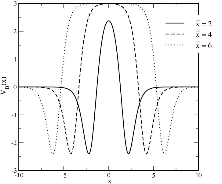
For computing the VPE, the large contribution from the constant but non–zero potential in the regime $|x|\lesssim\overline{x}$ should be eliminated. The above considerations lead to

$\displaystyle{\textstyle\frac{1}{2}}\lim_{\bar{x}\to\infty}\left\{E_{\rm vac}[V_{B}]-2E_{\rm vac}[V^{(2\overline{x})}_{\rm SB}]\right\}=-0.170\quad{\rm and}\quad{\textstyle\frac{1}{2}}\lim_{\bar{x}\to\infty}\left\{E_{\rm vac}[V_{B}]-2E_{\rm vac}[V^{(2x_{s})}_{\rm SB}]\right\}=-0.120\,.$

(38)

When the VPE from $V^{(2(\overline{x}+1.2)}_{\rm SB}$ is subtracted, the main result, Eq. (33), is matched. Eventually this can be used to define the center of the soliton.

Now we also understand why the VPE for $a\neq 0$ diverges as $a\to 0$, cf. table 2. In that limit kink and antikink structures separate and the ”vacuum” in between produces an ever increasing contribution (in magnitude).

Finally, we discuss the link between the translational variance and the Krein–Friedel–Lloyd formula, Eq. (8). We have already reported the VPE for the step function potential when $x_{m}=0$. We can also consider $x_{m}\to\infty$:

$\displaystyle\frac{E_{\rm vac}[V^{(x_{m})}_{\rm step}]}{|x_{m}|}\,\to\,$

$\displaystyle-{\rm sign}(x_{m})\,\left[\int_{0}^{\sqrt{3}}\frac{dk}{4\pi}\,\frac{2k^{2}-3}{\sqrt{k^{2}+1}}+\int_{\sqrt{3}}^{\infty}\frac{dk}{4\pi}\,\frac{2k^{2}-2k\sqrt{k^{2}-3}-3}{\sqrt{k^{2}+1}}\right]\approx 0.101\,{\rm sign}(x_{m})\,,$

(39)

reproducing the linear dependence on the position from above. Formally, i.e. without Born subtraction, the integral, Eq. (39) is dominated by

$\displaystyle\int\frac{dk}{2\pi}\,\frac{k}{\sqrt{k^{2}+1}}\left[k-\sqrt{k^{2}-3}\right]\sim\int\frac{dk}{2\pi}\,\sqrt{k^{2}+1}\frac{d}{dk}\left[\sqrt{k^{2}-3}-k\right]=\int\frac{dk}{2\pi}\,\sqrt{k^{2}+1}\,\frac{d}{dk}\left[q-k\right]\,.$

(40)

Essentially this is that part of the level density that originates from the different dispersion relations at positive and negative spatial infinity.

We have advanced the spectral methods for computing vacuum polarization energies (VPE) to also apply for static localized background configurations in one space dimension that do not permit a parity decomposition for the quantum fluctuations. The essential progress is the generalization of the variable phase approach to such configurations. Being developed from spectral methods, it adopts their amenities, as for e.g. an effective procedure to implement standard renormalization conditions. A glimpse at the bulky formulas for the heat kernel expansion (alternative method to the problem) in Refs.[14, 15, 16] immediately reveals the simplicity and effectiveness of the present approach. The latter merely requires to numerical integrate ordinary differential equations and extract the scattering matrix thereof, cf. Eqs. (18) and (22). Heat kernel methods are typically combined with $\zeta$–function regularization. Then the connection to standard renormalization conditions is not as transparent as for the spectral methods, though that is problematic only when non–local Feynman diagrams require renormalization, i.e. in larger than $D=1+1$ dimensions or when fermion loops are involved.

We have verified the novel method by means of well established results, as, e.g. the $\phi^{4}$ kink and sine–Gordon solitons. For these models the approach directly ascertains translational invariance of the VPE. Yet, the main focus was on the VPE for solitons in $\phi^{6}$ models because its soliton(s) may connect in–equivalent vacua leading to background potentials that are not invariant under spatial reflection. This model is not strictly renormalizable. Nevertheless at one loop order a well defined result can be obtained from the no–tadpole renormalization condition albeit no further finite renormalization is realizable because the different vacua yield additional infinities when integrating the counterterm. The different vacua also lead to different dispersion relations for the quantum fluctuations and thereby induce translational variance for a theory that is formulated by an invariant action. We argue that this variance is universal, as it is not linked to the particular structure of the background and can be related to the change in the level density that is basic to the Krein–Friedel–Lloyd formula, Eq. (8).

Besides attempting a deeper understanding of the variance by tracing it from the energy momentum tensor, future studies will apply the novel method to solitons of the $\phi^{8}$ model. Its elaborated structure not only induces potentials that are reflection asymmetric, but also leads to a set of topological indexes[28] that are related to different particle numbers. Then the novel method will progress the understanding of quantum corrections to binding energies of compound objects in the soliton picture. Furthermore the present results can be joined with the interface formalism[29], that augments additional coordinates along which the background is homogeneous, to explore the energy (densities) of domain wall configurations[30].

This work was presented at the $5^{\rm th}$ Winter Workshop on Non–Perturbative Quantum Field Theory, Sophia-Antipolis (France), March 2017. The author is grateful to the organizers for providing this worthwhile workshop.

The author declares that there is no conflict of interest regarding the publication of this paper. This work is supported in parts by the NRF under grant 109497.

References

- [1] T. H. R. Skyrme, Proc. Roy. Soc. Lond. A 260 (1961) 127.
- [2] T. H. R. Skyrme, Int. J. Mod. Phys. A 3 (1988) 2745, Article reconstructed by I. Aitchison.
- [3] E. Witten, Nucl. Phys. B 160 (1979) 57.
- [4] G. S. Adkins, C. R. Nappi, E. Witten, Nucl. Phys. B 228 (1983) 552.
- [5] H. Weigel, Lect. Notes Phys. 743 (2008) 1.
- [6] D. T. J. Feist, P. H. C. Lau, N. S. Manton, Phys. Rev. D 87 (2013) 085034.
- [7] F. Meier, H. Walliser, Phys. Rept. 289 (1997) 383.
- [8] F. G. Scholtz, B. Schwesinger, H. B. Geyer, Nucl. Phys. A 561 (1993) 542.
- [9] R. L. Jaffe, Phys. Rev. Lett. 38 (1977) 195 Erratum: [Phys. Rev. Lett. 38 (1977) 617].
- [10] A. P. Balachandran, A. Barducci, F. Lizzi, V. G. J. Rodgers, A. Stern, Phys. Rev. Lett. 52 (1984) 887.
- [11] N. Graham, M. Quandt, H. Weigel, Lect. Notes Phys. 777 (2009) 1.
- [12] M. A. Lohe, Phys. Rev. D 20 (1979) 3120.
- [13] M. A. Lohe, D. M. O’Brien, Phys. Rev. D 23 (1981) 1771.
- [14] A. Alonso–Izquierdo, W. Garcia Fuertes, M. A. Gonzalez Leon, J. Mateos Guilarte, Nucl. Phys. B 635 (2002) 525
- [15] A. Alonso–Izquierdo, J. Mateos Guilarte, Nucl. Phys. B 852 (2011) 696.
- [16] A. Alonso–Izquierdo, J. Mateos Guilarte, Annals Phys. 327 (2012) 2251.
- [17] E. Elizalde, Lect. Notes Phys. Monogr. 35 (1995) 1.
- [18]
E. Elizalde, S. D. Odintsov, A. Romeo, A. A. Bytsenko, S. Zerbini,
Zeta regularization techniques with applications, World Scientific, Singapore, 1994. - [19] K. Kirsten, AIP Conf. Proc. 484, 106 (1999).
- [20] H. Weigel, Phys. Lett. B 766 (2017) 65.
- [21] J. S. Faulkner, J. Phys. C, 10 (1977) 4661
- [22] N. Graham, R. L. Jaffe, V. Khemani, M. Quandt, M. Scandurra, H. Weigel, Nucl. Phys. B 645 (2002) 49.
- [23] E. Farhi, N. Graham, P. Haagensen, R. L. Jaffe, Phys. Lett. B 427 (1998) 334.
- [24] R. Calegero, Variable Phase Approach to Potential Scattering, Acad. Press, New York and London, 1967
- [25]
R. G. Newton,
Scattering Theory of Waves and Particles, Springer, New York 1982;
K. Chadan, P. C. Sabatier Inverse Problems in Quantum Scattering Theory, Springer, New York 1989. - [26] R. Rajaraman, Solitons and Instantons, North Holland, Amsterdam and New York, 1982.
- [27] G. Barton, J. Phys. A 18 (1985) 479.
- [28] V. A. Gani, V. Lensky, M. A. Lizunova, JHEP 1508 (2015) 147.
- [29] N. Graham, R. L. Jaffe, M. Quandt, H. Weigel, Phys. Rev. Lett. 87 (2001) 131601.
- [30] A. Parnachev, L. G. Yaffe, Phys. Rev. D 62 (2000) 105034.