A Quantum Model for Coherent Ising Machines:
Discrete-time Measurement Feedback Formulation

In the PSA, the signal pulse with an initial state $\rho$, frequency $\omega$, and annihilation operator $a$, interacts with the pump pulse, whose initial state is a coherent state $|\beta\rangle$ ($\beta$ is real) with a frequency $2\omega$. The pump pulse after the interaction is thrown away and in the next round trip, new pump pulse $|\beta\rangle$ is generated.

The amplitude $\beta$ of the pump pulse is very large and the interaction with the signal pulse is weak.

The Hamiltonian for the PSA is

Here, $B$ is defined as follows:

where $b(\omega_{k})$ is the annihilation operator of the pump field of frequency $\omega_{k}$, and $g(\omega_{k})$ is a parametric coupling constant. Initially, the pump field at $2\omega$ is in a coherent state $|\beta\rangle$ and all the other modes are assumed to be in vacuum state $|0\rangle$. When we displace the pump field as follows

the initial state of the pump field is displaced to a vacuum state. In this case, the Hamiltonian (1) is rewritten as

We shall interpret that the first term $\mathcal{H}_{s}$ represents the linear phase sensitive amplification/ deamplification (squeezing effect) imposed by the pump, while the second term represents up conversion process, which results in an effective two photon loss of the signal mode. The first part of the Hamiltonian can be absorbed as an internal Hamiltonian of the signal. Then, the second part is expressed as

in the interaction picture. We take the Born-Markov and the rotating wave approximations to eliminate the Hilbert space of the pump pulse. Then, we can find the master equation corresponding to the interaction Hamiltonian as follows [19] :

where

When we go back to the Schrodinger picture, we have

The first term in Eq.(7) represents a standard unitary (squeezing) process, while the second term is a Lindblad form representing the two photon loss process associated with the parametric pump photon generation. We defined the squeezing rate $S=g(2\omega)\beta t$ and the two photon loss rate $L=g(2\omega)^{2}t$, where $t$ is the time duration of this interaction in the PSA. The linear power-gain $G$ can be represented as $G=\exp(2S)=\exp(2g(2\omega)\beta t)$. One of the important assumption leading to Eq.(7) is that the gain saturation is relatively weak, i.e. the signal pulse intensity grows and depletes the pump power only slightly, instead of decaying to zero, as is the case for a traveling-wave PSA with strong signal-pump interaction [20]. The other important assumption is that the pump field is dissipated into external reservoirs each time of PSA and a fresh coherent state $|\beta\rangle$ is always prepared as a new pump field for the next round of PSA. The equation for our simulation is obtained by expanding the density operator $\rho$ in terms of the in-phase amplitude eigenstates $|x\rangle$ as follows:

where $z=x+x^{\prime}$ and $w=x-x^{\prime}$.

All coefficients which appears in the equation above are real-valued because annihilation and creation operators, which appear in the equation (7), are summation of in-phase amplitude operator $x$ and its derivative $\partial_{x}$ with real coefficients, which allows $\langle x|\rho|x^{\prime}\rangle$ are real-valued in CIM.

A portion of the signal pulse is extracted from the ring cavity by the two beam splitters. At the first output coupler, the extracted signal-field is simply dissipated in external reservoirs, which represents the background loss in the ring cavity. At the second output coupler, the in-phase amplitude $x=(a+a^{\dagger})/\sqrt{2}$ of the extracted field is projectively measured by the homodyne detectors. We define the transmittance of the first and second splitters as $T^{\prime}=\sin^{2}\theta^{\prime}$ and $T=\sin^{2}\theta$. When the signal pulse goes into the beam splitter, it is combined with the incident vacuum state from the external environments. Thus, the measurement performed by the homodyne detectors has a finite measurement error, which stems from the vacuum fluctuation. We define the annihilation operators of the signal and the vaccum field as $a$ and $a_{vac}$. Then, the output field annihilation operators can be written in terms of the unitary operator $U$ of the beam splitter with a parameter $\theta$ as follows:

From these equations, the Kraus operator corresponding to the measured value of $x_{m}$ can be expressed by

To calculate the conditional density matrix for the post-measurement state, we generate a random number and determine a measured value $x_{m}$ with the probability of $Tr(M_{x_{m}}\rho M_{x_{m}}^{\dagger})$. For the operation for the first output coupler, we use the same Kraus operators $\{M_{x_{m}}\}$ and ensemble many conditional density matrices governed by the probabilistically determined $x_{m}$.

In the feedback injection process, the signal pulse and feedback pulse, the latter of which is prepared in a coherent state $|\alpha\rangle$, are combined with a third beam splitter. The transmittance rate of the third beam splitter, defined as $T_{f}=\sin^{2}\theta_{f}$, is very high ($T_{f}\approx 1$). In this parameter region, the quantum flucutation due to the injected coherent state is much smaller than the flutucation in the signal pulse, and this feedback process can be described with a simple unitary displacement operator $D(\alpha\theta_{f})=\exp(\alpha\theta_{f}a^{\dagger}-\alpha^{*}\theta_{f}a)$. In the Heisenberg picture, the in-phase amplitude operator $x$ will be translated as $D(\alpha\theta_{f})xD^{\dagger}(\alpha\theta_{f})=x+\alpha\theta_{f}/\sqrt{2}$.

The amplitude $\alpha$ of the feedback pulse is determined by the measured values of the homodyne detectors. We define the feedback rate $R$ as the ratio of $\alpha\theta_{f}/\sqrt{2}$ to the in-phase amplitude $x$ of the signal pulse, estimated using the value $x_{m}$ measured by the homodyne detectors.

In summary, the signal pulses experience four processes described above during each loop around the ring cavity. The system is described by five physical parameters, the gain $G$ (or squeezing rate $S$), two photon loss rate $L$, background loss rate $1-T^{\prime}$ , measurement loss rate $1-T$, and feedback rate $R$. The total net linear amplitude-gain, before the gain saturation is switchwed on, during one round trip of the cavity is $G_{tot}=\sqrt{G\times T\times T^{\prime}}=\exp(g(2\omega)\beta t)\sin\theta\sin\theta^{\prime}$, where we assume that $T_{f}\approx 1$.

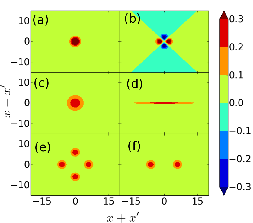
For numerical simulations, we expand the conditional density matrices of pulses in terms of $x$-eigenvectors and calculate the elements of the density matrices. Note that the elements of density matrices $\langle x|\rho|x^{\prime}\rangle$ are real numbers in this system. In this paper, we will visualize density matrices as functions of $x+x^{\prime}$ and $x-x^{\prime}$. While this function is equivalent to the Wigner function because Wigner function can be obtained by the Frourier transformation of $\langle x|\rho|x^{\prime}\rangle$ along the $x-x^{\prime}$ axis, it is easier to see the quantum coherence than Wigner function as shown in Figure 2.

Figure 2 shows the contour maps of the functions $\langle x|\rho|x^{\prime}\rangle$ corresponding to typical quantum states. The line of $x-x^{\prime}=0$ is the diagonal line of a density matrix and represents the probability distribution on $x$, while the line of $x+x^{\prime}=0$ represents quantum coherence between the element of $|x\rangle$ and the one of $|-x\rangle$. The vacuum state $|0\rangle$ and a one photon state $|1\rangle$ can be represented with a simple gaussian function whose variance is $\langle\Delta x^{2}\rangle=0.5$ and a phase reversed Hermite Gaussian function (Figure 2(a),(b)). When it is anti-squeezed along the $x$-axis, it becomes broader gaussian distribution (Figure 2(c)). On the other hand, a thermal state is a gaussian whose width is large along the $x+x^{\prime}$ axis but small along the $x-x^{\prime}$ axis (Figure 2(d)). This clearly shows the low qunatum coherence in the thermal state. While non-zero values appear along the vertical line of $x+x^{\prime}=0$ when two coherent states $|\alpha\rangle$ and $|-\alpha\rangle$ are superposed with quantum coherence, they disappear when the two coherent states are classically ensembled (Figure 2(e)(f)). These states shown in Figure 2 and states in our CIM model don’t have imaginary elements, so the functions can be described with contour maps of real values.

In this subsection, we assume that the background loss in the cavity is zero ($T^{\prime}=1$), and the transmittance of the output coupler is $T=0.99$. Thus, in this case, the ratio of power extracted from the cavity for the measurement is 0.01. Other numerical parameters are given in Table 1. Figure 3 illustrates the time-development of typical conditional density matrices of signal pulses governed by the sequence of measured values $x_{m}$. The initial states of the two pulses are vacuum states ( with the number of round trips $N=0$ in Figure 3 (b)). At that time, $\langle x\rangle=0$ and $\langle\Delta x^{2}\rangle=0.5$. The optimization process consists of three stages. In the first stage, the in-phase amplitudes of two pulses are anti-squeezed by the phase sensitive amplifier, and $\langle\Delta x^{2}\rangle$ become larger ($N=30$ in Figure 3 (b) ). Note that both the diagonal x-distribution along the horizontal axis and the off-diagonal quantum coherence plotted along the vertical axis become broad. In the second stage, because of the gain saturation and feedback processes, the expectation value $\langle x\rangle$ moves to either negative or positive value ($N=60$ in Figure 3 (b)). The gain saturation and the linear photon loss are responsible for the spontaneous symmetry breaking of DOPO, while the feedback process makes the system to select an anti-ferromagnetic order instead of a ferromagnetic order. Finally, in the third stage the state becomes close to the highly excited coherent state and $\langle\Delta x^{2}\rangle$ is reduced to $0.5$ ($N=150$ in Figure 3 (b) ). At this stage, the DOPO state is already in a classical level and the optimization process of the CIM is completed.

Next, we present the simulation results for various measurement strengths 1-$T$ under a condition of no background loss, $T^{\prime}=1$. The parameters for the numerical simulations are shown in Table 1. Figure 4 shows typical conditional density matrices $<x|\rho|x^{\prime}>$ governed by the sequence of measurement results $x_{m}$. It can be seen that the anti-squeezing effect at the early period of the optimization process is more significant when the transmittance of the output coupler is larger or the measurement strength is weaker so that the wavepacket reduction is not so significant. When $T=0.9$ or $T=0.5$, the states undergo mild anti-squeezing and they are quickly displaced. On the other hand, when $T=0.999$, the states maintains the quantum coherence between the macroscopically separated ”up state” and ”down state” ($N=60$ in Figure 4 (a)). Here, the probability distributions are not localized but the centers of the two wavepackets are negatively correlated. As shown in Figure 4(e), the Wigner function features an oscillatory behavior with negative amplitudes that manifests the quantum interference effect between the macroscopically separated ”up-state” and ”down-state”.

Figure 5 illustrates the relationship between $\langle\Delta x^{2}\rangle$ and $\langle\Delta p^{2}\rangle$ for a typical conditional density matrix and the full density matrix of a one signal pulse for various values of transmittance rate $T$. Here, $x,p$ are the in-phase and quadrature-phase amplitudes, respectively, defined by $x=\frac{a+a^{\dagger}}{\sqrt{2}},ip=\frac{a-a^{\dagger}}{\sqrt{2}}$. Initially at N=0, the state satisfies $\langle\Delta x^{2}\rangle=\langle\Delta p^{2}\rangle=0.5$. As the signal pulses complete many round trips around the ring cavity, the value of $\langle\Delta x^{2}\rangle$ for a conditional density matrix first becomes larger, and then decreases to $\langle\Delta x^{2}\rangle=0.5$ at well above DOPO threshold. These lines form loops. The dashed curve represents the minimum uncertainty product. The Heisenberg uncertainty principle dictates that $\langle\Delta x^{2}\rangle\langle\Delta p^{2}\rangle\geq 1/4$. Because the state is squeezed vacuum state in the early stage of the optimization process, it lies on this dashed curve when $\langle\Delta x^{2}\rangle$ is relatively small. The results depicted in Figure 5 clearly demonstrate the two facts. First, when the measurement strength is weaker, the states are more anti-squeezed and more quantum coherence is present between the ”up state” (the region $x>0$) and the ”down state” (the region $x<0$). Second, as $T$ becomes smaller or the measurement strength increases, the conditional density matrix becomes close to a squeezed coherent state, because the density matrix moves almost onto the curve of the minimum uncertainty product. In this case, the density matrices will be efficiently simulatable with the displaced squeezing basis method discussed in [21].

The degree of squeezing is more than 3dB in Figure 5 . It is well-known that a continuous wave (CW) pumped DOPO features only 3dB squeezing inside a cavity. However, such a limit does not exist for a pulsed DOPO. The numerical results shown in Figure 5(a)(b) are the uncertainty product at the input to the PSA, while that at the output of the PSA is shown in Figure 5(c).

After the many round trips of signal pulses, we projectively measure the in-phase amplitude of the pulses. If the amplitude is positive $x>0$, we treat it as a up-spin state, and otherwise, a down-spin state. Thus, in the case of two signals with out-of-phase coulping, the optimization by CIM is successful if the projectively measured in-phase amplitude of a signal is positive and the one of the other signal is negative. Thus, the definition of the success probability is $\int_{x_{1}x_{2}<0}\langle x_{1}|\langle x_{2}|\rho|x_{1}\rangle|x_{2}\rangle dx_{1}dx_{2}$, where $x_{1}$ and $x_{2}$ denote the in-phase amplitudes of the two signal pulses and $\rho$ is the full density matrix for the two signal DOPO pulses.

We produced many conditional density matrices, in order to calculate how the probability of success $P$ of the optimization depends on the background loss rate $1-T^{\prime}$, with the numerical parameters presented in Table 2 and three different pump schedules of net linear amplitude-gain $G_{tot}$. The results are shown in Figure 6.

The initial success rate for the two vacuum states is $0.5$ and as $N$ increases it becomes higher. To see the dependance of the probability of success on the background loss rate and the time schedule of the net linear gain, we set the feedback rate $R$ not to be sufficiently strong and $P$ does not reach 100%. Of course, when $R$ is sufficiently strong, $P$ reaches to 100%. In the case of a low background loss ($T^{\prime}=1.0$ and $0.9$), the initial increasing rate of $P$ is smaller than the case of a larger background loss. When the loss rate is low, the state is largely anti-squeezed, and this makes the signal-to-noise ratio of measurement is poor at the early stage, as shown in Figure 4. Thus, the in-phase amplitudes of the feedback pulses generated from the measured values suffer from small signal-to-noise ratio, and this leads to a lower increase rate for the probability of success at the early stage.

However, once $P$ starts to increase, it suddenly goes up and reaches to the final constant value. The final value greatly depends on the time shedule of the net gain $G_{tot}$. When $G_{tot}$ increases rapidly, the final probability of success for the low-loss case becomes lower than that in the case of slowly increasing $G_{tot}$. This is because the small fluctuation leads to the states of the DOPO pulses being easily trapped into the potential wells of DOPO (up-spin state or down-spin state) before the correlation between the two pulses permanently forms. On the other hand, when the background loss is large or $T^{\prime}$ is small ($T^{\prime}=0.5$ and $0.7$), the state fluctuates strongly and can move from the up (down) state to the down (up) state even after $G_{tot}$ becomes larger than one (above the threshold)[22] . Thus, the success rate continues to increase also in the later stage of the optimization process.

References

- [1] J. J. Hopfield and D. W. Tank, Biol. Cybern. 52, 141 (1985).
- [2] M. Ercsey-Ravasz and Z. Toroczkai, Nat. Phys. 7, 966 (2011).
- [3] E. Farhi, J. Goldstone, S. Gutmann, J. Lapan, A. Lundgren, and D. Preda, Science 292, 472 (2001).
- [4] T. Kadowaki and H. Nishimori, Phys. Rev. E 58, 5355 (1998).
- [5] E. G. Rieffel, D. Venturelli, B. O’Gorman, M. B. Do, E. M. Prystay, and V. N. Smelyanskiy, QIP 14, 1 (2015).
- [6] S. E. Nigg, N. Lörch, and R. P. Tiwari, Science Advances 3, e1602273 (2017).
- [7] S. Puri, C. K. Andersen, A. L. Grimsmo, and A. Blais, Nature Communications 8, ncomms15785 (2017).
- [8] H. Goto, Z. Lin, and Y. Nakamura, arXiv preprint arXiv:1707.00986 (2017).
- [9] Z. Wang, A. Marandi, K. Wen, R. L. Byer, and Y. Yamamoto, Phys. Rev. A 88, 063853 (2013).
- [10] K. Takata, A. Marandi, and Y. Yamamoto, Phys. Rev. A 92, 043821 (2015).
- [11] D. Maruo, S. Utsunomiya, and Y. Yamamoto, Phys. Scripta. 91, 083010 (2016).
- [12] A. Marandi, Z. Wang, K. Takata, R. L. Byer, and Y. Yamamoto, Nat. Photon. 8, 937 (2014).
- [13] J. Roslund, R. M. De Araujo, S. Jiang, C. Fabre, and N. Treps, Nat. Photon. 8, 109 (2014).
- [14] K. Takata, A. Marandi, R. Hamerly, Y. Haribara, D. Maruo, S. Tamate, H. Sakaguchi, S. Utsunomiya, and Y. Yamamoto, Sci. Rep. 6, 34089 (2016).
- [15] T. Inagaki, K. Inaba, R. Hamerly, K. Inoue, Y. Yamamoto, and H. Takesue, Nat. Photon. (2016a).
- [16] N. Treps, C. Jacquard, Y.-S. Ra, A. Dufour, F. Arzani, V. Parigi, and C. Fabre, in Frontiers in Optics (Optical Society of America, 2016) pp. FTh4F–3.
- [17] P. L. McMahon, A. Marandi, Y. Haribara, R. Hamerly, C. Langrock, S. Tamate, T. Inagaki, H. Takesue, S. Utsunomiya, K. Aihara, et al., Science 354, 614 (2016).
- [18] T. Inagaki, Y. Haribara, K. Igarashi, T. Sonobe, S. Tamate, T. Honjo, A. Marandi, P. L. McMahon, T. Umeki, K. Enbutsu, et al., Science 354, 603 (2016b).
- [19] H.-P. Breuer and F. Petruccione, The theory of open quantum systems (Oxford University Press on Demand, 2002).
- [20] R. Hamerly, K. Inaba, T. Inagaki, H. Takesue, Y. Yamamoto, and H. Mabuchi, Int. J. Mod. Phys. B 30, 1630014 (2016).
- [21] N. Tezak, N. H. Amini, and H. Mabuchi, arXiv preprint arXiv:1704.05369 (2017).
- [22] P. Kinsler and P. D. Drummond, Phys. Rev. A 43, 6194 (1991).