Delay Comparison of Delivery and Coding Policies in Data Clusters
Abstract
A key function of cloud infrastructure is to store and deliver diverse files, e.g., scientific datasets, social network information, videos, etc. In such systems, for the purpose of fast and reliable delivery, files are divided into chunks, replicated or erasure-coded, and disseminated across servers. It is neither known in general how delays scale with the size of a request nor how delays compare under different policies for coding, data dissemination, and delivery.
Motivated by these questions, we develop and explore a set of evolution equations as a unified model which captures the above features. These equations allow for both efficient simulation and mathematical analysis of several delivery policies under general statistical assumptions. In particular, we quantify in what sense a workload aware delivery policy performs better than a workload agnostic policy. Under a dynamic or stochastic setting, the sample path comparison of these policies does not hold in general. The comparison is shown to hold under the weaker increasing convex stochastic ordering, still stronger than the comparison of averages.
This result further allows us to obtain insightful computable performance bounds. For example, we show that in a system where files are divided into chunks of equal size, replicated or erasure-coded, and disseminated across servers at random, the job delays increase sub-logarithmically in the request size for small and medium-sized files but linearly for large files.
I Introduction
Modern cloud computing infrastructures feature several clusters each of which consists of thousands of highly interconnected servers which collectively run and serve diverse computing applications [1, 2, 3]. An important aspect of these clusters is to collectively store and deliver Internet scale data/files. Key design challenges for such systems include placement of files across servers and an algorithm for the swift delivery of dynamically arriving file requests. A common practice towards file placement is to divide each file into chunks of fixed size, which could then potentially be replicated/coded, and to disseminate them across the servers [4, 5]. This can potentially reduce delays in delivering large files since the delivery algorithm could now aggregate the service rate from multiple servers.
To gain intuition, consider some hypothetical scenario where, for the placement of each file, one is allowed to use variable and arbitrarily small (possibly fractional) chunk sizes. Then, for a system of servers, one could divide each file of size bits into different chunks, each of size bits. Suppose that the service/delivery rate at each sever is bits/sec and that there is no other network bottleneck. Then, the minimum achievable delay in serving a download request for a file of size is , which is possible only if no other request is present in the system.
However, delays which scale inverse linearly with clearly cannot be achieved for each file if there is a limit to the minimum chunk size. For example, suppose that each file of size is divided into chunks of size . Then, if there is only one download request in the system at a given time, for any file of size less than , a download delay equal to can be achieved. Whereas for files several times larger than bits, the delay is still of the order of under isolation. However, for a system with diverse files and fixed chunk size, it is not directly clear what the delays are under stochastic loads. In such a setting, how do delays relate with the size of a requested file? Do replication of chunks or erasure coding help in reducing delays? What is the impact of dynamic load-balancing? These are some of the questions we address in this work.
Contributions: We provide a stochastic model which encapsulates the key features of the content delivery process in a highly interconnected cluster of servers and allows us to compare several different policies as well as to obtain explicit performance bounds. In particular, our model captures the following aspects:
Dissemination policy: We allow each file to be divided into chunks of a given size. Thus, a larger file is divided into larger number of chunks. These chunks are most often encoded to obtain code blocks of the given size, as explained below. The code blocks are then disseminated across servers in a randomized fashion to ensure that the load across servers is balanced.
Coding policy: Suppose that a file is divided into chunks. For each , these chunks are coded into code blocks for some via MDS (maximum distance separable) erasure codes [6, 7]. These codes are designed such that the original chunks can be exactly recovered from any out of the code blocks. This allows additional flexibility towards dynamically balancing load across servers as the requests arrive over time, as explained below.
Delivery policy: Upon the arrival of a request for a file with chunks, a request is sent to a subset of servers to obtain out associated code blocks. The servers serve the block requests in FCFS fashion. We allow dynamic load balancing policies such as Water-filling and Batch Sampling policies (defined below) which favor a subset of the set of servers with lower instantaneous loads to balance the server workload as well as to achieve lower request delays.
We propose a comprehensive model for this class of systems, with the potential of representing all such policies under certain diversity and symmetry assumptions on the file sizes and the loading policy. This model consists of a set of evolution equations which allow for both efficient simulation and mathematical analysis under general statistical assumptions. In particular, we are able to show the following:
- 1.
We compare the evolution of workloads under three different delivery policies: namely, water-filling (), batch sampling (), and a randomized policy called Balanced Random (). We show that, for a given workload at each server, is optimal in the sense that upon a new arrival, it achieves ‘the most balanced’ workload as compared to any other policy. Further, is somewhere in between and in this respect.
- 2.
We show that and achieve more favorable workload distributions and lower delay distributions as compared to in the sense of ‘increasing convex order’, which in turn implies that the former policies achieve better performance not only in expectation but in higher moments as well.
- 3.
We provide an upper bound for the delay in delivering a file as a function of its size, under a scenario where the requests form a mix of diverse file sizes. Our bound reveals the relative impact of the local dynamics at an individual server and that of the global view of server workloads seen by an arrival. We also provide new scaling laws on the behavior of delays under such a scenario.
- 4.
Using simulations we analyze the impact of the key options and parameters, including the delivery policy, the coding options and the chunck size. We identify two fundamental regimes, the logaritmic regime when the file sizes are such that no two chunks are stored on the same server, and the linear regime when files have a number of chunks that exceeds the number of servers. We show that in the logarithmic regime, the gains of dynamic load balancing via and are significant even when the coding rate is small. We also show that our product form bound on the delivery latency is tight when requests have a moderate size.
Related Work: Recently there has been significant interest towards developing scalable performance models and analysis for content delivery systems with low delays. For example, the work in [8, 9, 10] exploits server parallelism via “resource pooling”, that is multiple servers are allowed to work together as a pooled resource to meet individual download requests. The pools of servers associated with different requests may overlap, so the sharing of server resources across classes is done via a fairness criterion. Under a scenario where the size of resource pools is limited (i.e.), it is shown that the gains of resource pooling and load-balancing can be achieved simultaneously.
An alternate approach considered in the literature is to split a download request into multiple parts, for example, into requests for individual chunks, and achieve server parallelism by employing different servers for different parts [11, 12]. Further, sophisticated coding policies are employed to achieve flexibility in server choices [12]. Under the assumption that the number of servers available for each request is limited, the works in [11, 12] are able to use mean-field based arguments to study performance as the number of servers tends to infinity. Several other works also study queuing models under coding based techniques via heuristics or bounds, e.g.[13, 14, 15, 16], but these are not scalable for our purposes.
We depart from the above approaches in that we are interested in developing performance models for a regime where we obtain a maximum gain from server parallelism without restricting ourselves to limited resource pools or a limited number of available servers for each request. Given a lower bound on the chunk size, we divide each file into a maximum number of chunks and disseminate them across several servers, potentially servers for large files. Thus, we allow servers to take care of a request in parallel. We allow diverse file sizes and provide a delay bound which is a function of the file size.
In terms of tools used, we model the system dynamics via an evolution equation which is a generalization of the Kiefer and Wolfowitz recursion for workloads in queues [17], which allows us to go beyond exponentiality assumptions for file-size requests. We use coupling arguments to compare different policies. Coupling has been used to compare several queueing systems in past, e.g., see for example [10, 18]. Further, to provide explicit bounds on delays, we use the notion of association of random variables, which is a property that has had several applications in queueing systems and beyond [17, 19].
Organization: In Section II we provide our system model and develop the evolution equations. In Section III we provide results comparing various dynamic load balancing policies via coupling arguments. In Section IV we give performance bounds based on the notion of association of random variables. In Section V we consider a scenario where the chunk size may be different for different files. In Section VI we provide simulation results and numerical evaluations. We conclude in Section VII. Some proofs of technical nature are provided in the Appendix.
II System Model
We consider a system with servers, indexed . The system consists of a very large number (several orders of magnitude larger than ) of diverse files. We assume that the size of each file is an integer multiple of bits. Each file is divided into chunks of size bits each. These chunks are encoded before being placed across servers, as explained below.
For each positive integer we use an MDS erasure code of rate , where is an integer greater than or equal to . Such a code is called MDS code in coding theory [6]. Thus, equivalently, each file of size is divided into chunks and encoded into code blocks of size bits each. The MDS erasure codes may serve various practical purposes. Only the following property is relevant for our purposes: for a file of size , it is possible to recover the entire file by downloading any out of the code blocks.
For each file of size , the associated code blocks are placed across servers as follows. If , then we choose among the servers uniformly at random and place a distinct code block across each of these servers. Else, we place distinct blocks on each server and for the remaining blocks we choose that many servers uniformly at random.
We assume that the blocks are placed across servers as described above at time . The placement of blocks is kept fixed since then. From time , file download requests arrive as per an independent Poisson point process with rate . Let be the points of .
Consider a probability mass function . Each request arrival corresponds to a file of size bits with probability independently of all other arrivals. Let be the number of chunks for the file requested at time . Thus, is a sequence of discrete i.i.d. random variable with p.m.f. .
For each , let represent the placement of the file requested at time , in the following sense: for each server the entry represents the number of coded blocks placed on server that correspond to the file requested upon the arrival. Thus, for each , if , then . We call the sequence of placement vectors.
Let denote the mean file-size in bits. Let denote the per server load in bits/sec.
Assumption 1 (Symmetry in load across servers)
Due to the randomized placement of blocks, for a very large number of files, the load across servers is approximately symmetric. Thus we model the symmetry in load via symmetry in request arrivals as follows: given , is chosen uniformly at random from each of its feasible realizations. Equivalently, given , the entry is equal to for servers chosen uniformly at random and it is equal to for the rest of the servers.
Making such a symmetry assumption to obtain insightful results is a common practice, see e.g. [11, 8, 12]. While, in general, a system with a finite number of files may not be symmetric, we believe that this is a good approximation especially when the number of files is an order of magnitude larger than the number of servers.
We will not discuss server memory capacity issues here as this is not needed. Note however that such a randomized placement results into concentration of memory usage at each server.
Delivery policy: Upon each arrival, we load servers with requests for coded blocks via a delivery/routing policy as described below. Each server serves its block requests in FCFS fashion at rate , i.e., it delivers a code block at the rate of bits per second. Recall, due to our use of MDS codes, if then the system only needs to deliver out of the associated blocks for the arrival. We let denote the valued random variable where is the number of blocks requested from server upon the arrival. Thus, we have and for each . We call the sequence of routing vectors. Following are some of the admissible routing policies, each resulting into possibly different sequences of routing vectors.
Balanced Random Policy (): For each , if , then request blocks from each server and, for the remaining blocks, choose the same number of servers at random from the remaining servers having an additional block. More formally, suppose . Let and . From the set choose a subset of size at random. Let be equal to for each in this subset and for others.
The following two policies take a routing decision upon the arrival based on the instantaneous workloads at different servers at time .
Batch Sampling Policy (): This is a workload dependent policy. The workload at a server at any given time is the number of bits requested from the server and which are not yet served. Of the required blocks, request blocks from each server and for the remaining blocks, choose the servers with least instantaneous workload from the remaining servers having an additional block. More formally, suppose that the workload at the servers at time is and that . Let and . Let be given recursively as follows: let , and for let Then, we have for each and for .
Water-filling Policy (): This is also a workload dependent policy. If , then at time , we take a routing decision for block requests defined sequentially as follows. Among the servers which store at least one of the blocks for the associated file, choose the server with minimum workload. If there are multiple such servers, choose one at random. Request a block from this server and update its workload, i.e., add to its existing value. We now have to choose blocks among the remaining code blocks, for which we repeat the above procedure, see Fig. 1.
More formally, suppose that the workload at the servers at time is and that . Then, let be recursively given as follows: , and for let
For , let represent the vector in with entry equal to and other entries equal to . Then, under the policy we have .
One would guess that is the most egalitarian policy, i.e., it attempts at spreading the arriving load to servers with lower instantaneous workloads, and is somewhere in between and in egalitarianism. We will corroborate these intuitions in the next section.
Note that we do not allow policies which depend explicitly on the server indices. More concretely, if server indices are permuted at time , the choice of servers upon each arrival is permuted in the corresponding fashion.
Recall that the routing vector for each is such that is chosen independently with distribution , while its entries depend on the workload at the servers at time and on the delivery policy. Due to symmetry in file placement (modeled via symmetry in request arrivals) and the above mentioned restriction on the delivery policies, we have that are exchangeable random vectors in the following sense: upon permutation of server indices the distribution of the sequence remains unchanged.
Let be inter-arrival times, i.e., for each . Let be a sequence of valued random variables representing the workload seen by arrival, i.e., the workload at different servers at time . Then we have and
| (1) |
where , and
The delay of the request is then:
As mentioned earlier, we are mainly interested in the case where is a constant since we want to obtain a maximum gain from server parallelism. However, one can envisage a scenario where different requests/files use different chunk sizes. This can be incorporated in our model as follows: we have and
| (2) |
where the random variables are valued and i.i.d.. Note that in this extension, for a given file, the chunks are still of equal sizes. For most parts of the paper, we will use recursion (1). We will nevertheless discuss and analyze (2) in Section V.
III Comparison of Delivery Policies
In this section we compare the server workloads and the request delays under different delivery policies. We use coupling arguments to compare systems adopting different delivery policies. In particular, we couple the request arrival process as well as the sequence of routing vectors in each system. We then study and compare the evolution of server workloads in the respective systems.
For comparing the workloads of different systems, we use stochastic submajorization and stochastic dominance in the increasing convex order sense, which are briefly introduced in the first subsection. While the former is more amenable to compare the loading under different policies subject to a given initial condition, the later allows us to propagate the comparison result and also to compare delays (recall that the delay of a request is the of the delays in downloading individual blocks).
III-A Order statistics and stochastic orders
For all vectors , let represent its entries in increasing order.
We say that a function is symmetric if for all and its permutation , we have .
For two vectors , we say that is majorized by , which is denoted by , if and for . Intuitively, if , then is ‘more balanced’ than . For example, in , we have .
We say that is submajorized by , which is denoted by , if for .
We say that a function is Schur-convex if, for all and such that , we have . One can check that a function is Schur-convex and increasing if and only if (iff), for all and such that , we have . Further, Schur-convex functions are symmetric since the property depends only on the ordered entries of and .
Consider two random vectors and . We say that is stochastically dominated by , which is denoted by , if, for all increasing functions , we have . A classical result (Strassen’s theorem) states that iff there exist random vectors and such that and are identically distributed, and are identically distributed, and w.p. .
For two random vectors and we say that is stochastically submajorized by , which is denoted by if, for all Schur-convex functions , we have . We have iff there exist random vectors and such that and are identically distributed, and are identically distributed, and w.p. .
Similarly, for the random vectors and we say that is stochastically submajorized by , which is denoted by , if, for all increasing Schur-convex functions , we have . Again, iff there exist random vectors and such that and are identically distributed, and are identically distributed, and w.p. .
For the random vectors and , we say that is stochastically dominated by in the increasing convex order sense, which is denoted by , if, for all increasing convex functions , we have .
For , let denote the vector in with entry equal to and other entries equal to . For any vector we let represent the sum of the absolute values of its entries.
The following lemma is proved in the Appendix.
Lemma 1
Consider valued exchangeable random variable and . If then we have .
III-B Comparison of Policies
A delivery policy can be seen as a form of load balancing. Intuitively, a more egalitarian load balancing should achieve more balanced overall workloads. For instance, recall the policies , , and defined in the System Model. The following theorem says that, given a workload vector , is the most egalitarian policy while is somewhere in between and . For a proof, see the Appendix.
Theorem 1
Suppose an arrival into the system sees the workload , where is an valued random variable. Let , , , and be the routing vectors associated with , , , and an arbitrary routing policy, respectively. Then, the following holds.
Further, if is an exchangeable random vector, then we have
Thus, for a given workload at , a system under or achieves a more balanced workload in the sense at as compared to . However, the resulting workloads might be different. Starting with , to be able to claim that an ordering holds for each , one needs to argue that it propagates. For this we additionally need the monotonicity property of given in the lemma below. For a proof, see the Appendix.
Lemma 2
Consider random vectors and such that . Let and be the routing vectors as per the policy for and respectively. Then,
The following theorem establishes that the and policies achieve ‘more balanced and lower’ workloads across servers as compared to in a strong sense. For a proof, see the Appendix.
Theorem 2
Consider a system which starts empty. The workload under policies , , and satisfy the following:
Proof:
We show the comparison result for a system with and a system with ; the argument for comparison for and is analogous.
Suppose that the two systems are fed with arrivals as given by the same point process . Thus, the sequence of interarrival times is the same for both systems.
For ease of notation let represent the vectors associated with with their usual meaning, and let represent those associated with . holds trivially since both systems start empty. Now suppose that for a given . We show below that this implies .
From Theorem 1 we have that . Further, by Lemma 2 we have . Thus, we have . Since has equal entries and is an increasing and convex operation, we have , i.e., . Hence the result holds. ∎
The above theorem implies, for example, that each raw moment of the workload at given server under and is less than or equal to that under . Similarly, each raw moment of the total workload in the system is lower or equal under and as compared to that under .
However, the above theorem does not directly allow us to compare the delays of requests for each . To see this, recall that delay seen by a request is the of the delays in downloading individual blocks, which are random in number. Further, a more unbalanced workload may have more empty servers than . The next arrival could, for example, have the associated blocks stored on the servers which are empty in and not in .
The following theorem compares delays of requests under both the policies.
Theorem 3
Consider a system which starts empty. The delays seen by requests under the , , and policies satisfy the following:
Proof:
We show this for ; the argument for is analogous.
For ease of notation, we will use the notation for random vectors associated with policy with their usual meaning, and for those associated with policy .
For a given valued vector , the function is increasing and convex in . Thus, for any increasing convex function , is an increasing convex function in . Thus, from Theorem 2 we have E_s’_ng(max_i: s^′i_n ¿ 0 (W_n^i+c s^′i_n) ) ≤E_s’_ng(max_i: s^′i_n ¿ 0 (W_n^′i+c s^′i_n) ), where denotes the conditional expectaion given . Note that on both sides of the above inequality we are conditioning on which is the routing vector associated with .
Recall that under the policy, is independent of the instantaneous workload for each . Using the coupling and , and the definition, given instantaneous workload one can additionally couple the routing vectors and and the associated block requests under and policies such that the workload seen by the block in front of it under is lower than that under for each under . Thus, we get E_s’_ng(max_i: s^i_n ¿ 0 (W_n^i+ cs^i_n) )≤E_s’_ng(max_i: s^′i_n ¿ 0 (W_n^i+c s’^i_n) ). By combining the previous two inequalities we get E_s’_ng(max_i: s^i_n ¿ 0 (W_n^i+cs^i_n) ) ≤E_s’_ng(max_i: s^′i_n ¿ 0 (W’_n^i+c s’^i_n) ) , from which the result follows by taking expectation on both sides. ∎
Recall that is the load factor per server. The overall system load is . By exchangeability, the marginal dynamics of the workload at a given server under can be modeled via an FCFS queueing system with load bits/sec and service rate bits/sec. Since the number of servers is finite, the system is stable (asymptotically stationary) if . From Theorem 2 and the ergodicity of the arrival process, it follows that the system is stable under and as well if .
Note that, for general , the delays under the policy are statistically equivalent to the delays obtained when for each , i.e., when the code rate is equal to . There are prior works which study gains of erasure-coding via simulations [13, 14], experiments[15, 16], and analytically but under mean-filed type asymptotic approximations and under exponential service time assumptions [12]. To the best of our knowledge, Theorem 3 is the first rigorous analytical result which compares delays for finite systems employing erasure codes with different code rates. Further, we would like to stress that the result holds under general statistical assumptions for service requirements.
IV Association and Delay Bounds
In this section, we use the notion of association of random variables to obtain computable bounds on the delays of requests.
Definition 1
The random variables are associated if, with notation , the inequality
holds for each pair of increasing functions for which , , and exist.
We say that a random vector is associated if its entries are associated. Similarly, we say that a set of random variables is associated if its elements are associated.
To understand the power of association, consider the following definition and subsequent proposition.
Definition 2
Consider random variables . We say that are independent versions of the random variables if the are mutually independent, and if and are identically distributed for .
Proposition 1 (see [17] Chap 4.3)
Suppose that random variables are associated and that are their independent versions. Then the following holds:
Now consider different queues with dependent workloads, as in the previous section. If we can show that the arrival of a request sees associated workloads, then we can bound its delay by using the independent version of the workloads. Several works in the literature for large-scale systems, e.g. [21, 12], consider the marginal distribution at a given server and study its properties by assuming that the dynamic at any other server is independent of that under the given server; an assumption which is justified in these works as a ‘mean-field approximation’. In [21], the queue associated with a given server is called a ‘queue at the cavity’. With the association property, can analyze a system without resorting to the mean-field approximation.
Recall that under the policy, the selection of servers is independent of the workload . Upon an arrival, a server gets no additional workload with probability , and gets workload which is a multiple of otherwise. One can show that, given that the request is of size , the server gets the load with probability and the load with probability . Thus, for , the workload process at server, namely , in isolation is stochastically equivalent to workload seen by arrivals in a Cavity Queue which is as defined below.
Definition 3
A Cavity Queue is an FCFS queue which starts empty at time , has Poisson arrivals with rate , service rate bits/sec, and service requirement in bits with probability mass function on set given as follows:
and for
The FCFS queues are well studied in the literature. In particular, the following lemma well-known as Pollaczek-Khinchine formula describes the steady state workload distribution of jobs in these queues. Below, we view service time of a job as the ratio of its service requirement in bits and the service rate of the server in bits/sec.
Lemma 3 ([22])
Consider an FCFS queue with arrival rate . Let be a random variable with distribution equal to that of the service times of jobs. Let . Suppose that . In steady state the workload has Laplace Transform (i.e., ) which can be given as:
| (3) |
Below, we use (3) to obtain performance bounds on the systems of our interest by using association property along with Proposition 1. The following subset of the many known properties of association can come handy in proving association of random variables (RVs).
Proposition 2 (see [17] Chap 4.3)
The following statements hold.
- (i)
The set consisting of a single RV is associated.
- (ii)
The union of independent sets of associated RVs forms a set of associated RVs
- (iii)
Any subset of a set of associated RVs forms a set of associated RVs
- (iv)
For a non-decreasing function and associated RVs , the random variables
are associated.
Before providing our main results for this section, we need the following additional notation.
Definition 4
For each , let denote the delay seen by the arrival given that the size of the requested file is bits, that is,
| (4) |
Recall that for each , the request for a file is of size bits with probability and the requests for coded blocks are routed to different servers upon the arrival as per the chosen policy.
Definition 5
Let be the class of probability mass functions such that for each in class , a system with servers operating under policy has the routing vector which is associated for each .
In this paper we will be content to note that is a rich class of p.m.f.s which includes distribution as well as distribution for each .
The following theorem, proved in the Appendix, says that for any in , we get an upper bound on the delay seen by the arrival by pretending that the workloads at the servers ‘evolved independently in the past’.
Theorem 4
Consider a system with servers which starts empty. For each , requests for files of size bits, equivalently batch requests for blocks of bits each, arrive as per an independent point process with rate and are routed to different servers upon arrival. Servers serve the block requests in FCFS fashion at rate bits per second.
Suppose that belongs to class (see Definition 5). Then the following statements hold:
- 1.
The workload , at the servers seen by the arrival under is associated for each .
- 2.
Here is now a uniform bound in .
Theorem 5
Consider a system satisfying the assumptions of Theorem 4. Suppose that . For , let represent the stationary workload of an independent Cavity Queue. Then, under either , , or , the conditional delay satisfies the following property: for each :
| (6) |
Proof:
This follows from Theorem 4 and noting that, using standard coupling arguments, an queue starting empty at time and its version in equilibrium can be coupled in such a way that the former is always lower than the latter. ∎
The above bound clearly reflects the impact of the local dynamics at individual servers as well as the global view seen by arrivals. As we shall see, it can be computed using Lemma 3 and using extremal statistics.
In what follows, we focus on such that for each . Such a case is perhaps meaningful for clusters with very large since files which span each of the thousands of servers may be rare. Under this scenario, Corollary 2 below shows that delays admit a particularly simple bound.
Corollary 1
Consider a system with servers. Suppose that belongs to class and that for each . Suppose that . Let
| (7) |
where denotes the principal branch of the Lambert W function. Then, under , or , the conditional steady state delay satisfies
| (8) |
as tends to infinity, where is the function defined in (7).
Note that the last relation implies that
when tends to infinity. However it turns out that the formulation in (10) is numerically more accurate in the prelimit.
Surprisingly, as long as belongs to and the load per server is fixed, the above bound does not depend on . However, note that the bound is for the conditional delay. The bound on the overall delay still depends on .
V Random Chunk Sizes
We now study the scenario where the chunk size may be different for different files, which is modeled via recursion (2). Suppose that the random variables are i.i.d. with distribution . The results of Section III readily extend to this scenario. In particular the statement of Theorems 1, 2 and 3 can be shown to hold for this scenario as well, with minor modifications in the proofs. We skip the details for brevity.
We now extend the results of Section IV. We first modify the notion of Cavity Queue as follows.
Definition 6
The Modified Cavity Queue is an FCFS queue which starts empty at time , has Poisson arrivals with rate , service rate bits/sec, and where service requirement in bits are i.i.d. with distribution equal to that of the random variable , where can is generated as follows: first, generate a valued random variable with probability mass function given as follows:
and for
Let be a random variable with distribution . Then, .
Recall that the steady state workload distribution of an FCFS queue satisfies Lemma 3. By using the above notion of Modified Cavity Queue, analogues of Theorem 4 and 5 can be shown to hold with minor modifications in proofs. Here, we only reproduce the analogue of Theorem 5 for brevity.
Theorem 6
Consider a system with servers which start empty. The chunk sizes are i.i.d. with distribution . For each , batch requests for blocks (i.e., coded chunks) arrive as per an independent point process with rate and are routed to different servers upon arrival. Servers serve the block requests in FCFS fashion at rate bits per second.
Suppose that belongs to class (see Definition 5). Suppose that . For , let represent the stationary workload of an independent Modified Cavity Queue (see Definition 6). Then, under either , , or , the conditional delay satisfies the following property: for each :
| (9) |
where is a random variable with distribution .
Again consider a scenario where for each . Suppose that is exponential. Then the Modified Cavity Queue is an queue. Thus, the following corollary readily follows from the above theorem.
Corollary 2
Consider a system with servers. Suppose that belongs to class , and that for each . Suppose that the distribution is exponential with mean . Suppose that . Then, under , or , the conditional steady state delay satisfies
| (10) |
VI Simulation and Performance Evaluation
In this section we use our analysis and simulations in order to develop a better quantitative understanding of the relative performance and scaling laws under , , and .
VI-A Simulation Methodology
The simulation methodology we selected is not based on the classical discrete event principles but rather on a direct use of the recurrence equations (1). The advantages of the latter on the former are multiple, in term of generality and of complexity. This recurrence relation setting is well adapted to handling deterministic service times and general routing vectors, whereas event driven Markov chain simulation would require exponentiality assumptions and make the handling of workload based routing policies cumbersome. The complexity of is that of a sorting algorithm. If the servers containing at most one chunk from the requested file are sorted in increasing order of their load, then it suffices to take the smallest loads if . When , the complexity depends on rather than , as only servers with the smallest load need to be searched. The complexity is then in . The complexity of depends on whatever its value: one strategy is to first sort the servers containing at least one chunk of the requested file. Each time a chunk is requested from one server, its load increases by , and this server has to be re-inserted in the ordered list of servers. The complexity is then .
In several experiments, the size of the files is at most and . When for all , then and are exacly the same: as each server contains at most one chunk of any given file, all the routing vectors are balanced, and Theorem 1 states the optimality of in this case. For this reason, we will only compare with .
An important question is that of the steady state characterization. For this, we leverage Birkhoff’s pointwise ergodic theorem, which shows that empirical averages based on iterates of the recurrence equations (1) converge to the steady state mean values. In practice, we perform iterates to estimate each point of the following plots.
VI-B Impact of the Delivery Policy
The first numerical experiments illustrate the comparison results of Section III and more precisely Theorem 2. The setting is the following: there are servers; the distribution is Binomial, with (which gives an average of 20, 60 and 100 chunks, respectively); recall that for each value of this falls within the class of distribution ; the server speed is and the chunk size is ; the arrival rate is chosen in such a way that the load per server is always equal to 0.7; the coding assumptions are that .
Figure 2 compares the mean delay under and , for various values of . The bound obtained in Corollary 2 is also plotted. Within the range considered in these plots, the mean delays increase logarithmically in for . The bound correctly captures the logarithmic increase w.r.t. the , and is in fact approximate for small . For these parameters, it is already a good heuristic for .

We observe that (or equivalently ) performs significantly better than . Intuitively, this happens since the workload across servers is more balanced under and . In particular, while they seem to increase as for and . One may see this in the light of the well-known result on balanced allocations under balls and bins setting [23] where load-balancing is shown to achieve exponential improvement in load at the most-loaded bin. However, our setting is markedly different. Not only do we incorporate queuing dynamics (i.e., arrivals and services), but also batch arrivals. We are interested in studying the delay of a typical job which depends on the workload at a randomly chosen subset of servers, instead of the most-loaded server.

Interestingly, in our setting, the increase in delays seems logarithmic in even for and policies under a scenario where the chunk size is assumed to be random, as exhibited in Figure 3. The setting is the following: there are servers; the distribution is Geometric with rate , the size of chunks are exponentially distributed with rate . The load per server is . The coding assumptions are that . The plots show that, in the cases where the chunks sizes are exponentially distributed, the growth in delays as exhibited by the upper bound of Corollary 2 is tight when the per-server load is sufficiently large.
Under the assumptions studied above, for each policy, the growth of delays is logarithmic or sub-logarithmic in the file size. This type of growth does not generalize to all cases. For instance, it is shown in Subsection VI-E below that it can actually be linear.
VI-C Impact of Coding Rate
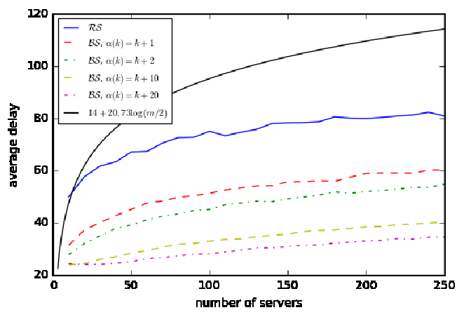
In order to evaluate the impact of coding rate, we consider a system under with servers, where varies. We take , and again is Binomial, so that the load per server is constant. We take and . Figure 4 gives the mean delay as a function of for different choices of .
As expected, and perform significantly better than when . We observe that the delays increase logarithmically with . This may be reasoned as follows: In the presence of small and medium sized files if is a constant then the choice in load-balancing is limited and the unevenness in workload distribution across servers increases with . Further, as we increase the code redundancy , we observe that the mean delays decrease as . This shows that the impact of increasing choice in load-balancing by improving coding rate is limited.
VI-D Impact of the (Deterministic) Chunk Size
We now consider the impact of increasing chunk size on delays for the case with being Binomial. Rather than taking chunks of size , we take chunks of size with an integer larger than 1, and study mean delay as a function of . Here, a file which had chunks now has chunks. Consider the upper bound of Corollary 2 (this bound is generic in that it holds for all considered delivery policies). The bound in the new chunk definition is now , when tends to infinity, with the only negative solution of the equation When is large (but such that ), this root can be approximated as so that we have the generic bound on requests of initial cardinality :
when tends to infinity. This shows that within the above Binomial setting, the mean delay of any policy can be decreased in such a way that the constant multiplying the logarithmic term is divided by (provided ).
VI-E Beyond the Logarithmic Regime
The last three subsections were about the case where has its support on the integers from 0 to . In view of the results of these subsections, it makes sense to call this regime the logarithmic regime. There are some caveats with this terminology. This term is justified within the setting, if is sufficiently separated from 1. As we saw above, for constant and less than 1, the logarithmic regime prevails even when tends to infinity. Note that this goes way beyond the regimes considered in the mean field approach. However, it should be clear that for fixed and for close to 1, the mean delay must be approximately a constant in .
Note that when the support of is not limited to the integers less than with fixed, it should be clear that for all delivery policies, when tends to infinity, requests of cardinality have a mean delay of order with a constant. This is the linear regime alluded to above.
VII Conclusions
One of the main motivations of this work was to derive scaling laws for job delays in data clusters. A primary difficulty in the analysis of job delays in multi-server systems comes from the stochastic coupling of the server dynamics. To simplify the analysis, research often resorts to an asymptotic ‘mean-field’ approximation which assumes an infinite number of servers and a static empirical distribution. This approximation allows for the decoupling of the dynamics at the servers attending a tagged job. However, such a decoupling does not hold when the total number of servers is finite, or when certain jobs are attended by servers. In the present paper, we developed a new machinery which utilizes the notion of association of random variables to obtain explicit bounds on delays for finite systems. We obtain these bounds via an ‘independent version’ of a coupled system but without requiring the decoupling of the servers. Further, we clarified the sense (increasing convex ordering) in which adaptive policies outperform workload oblivious policies. Our simulation results suggest that several quite different delay growths can be obtained in function of file size, from strictly sub-logarithmic to logarithmic to linear. While some specific examples of these behaviors are well explained by our machinery, there is still a need in the future for a full classification allowing one to predict which assumptions lead to each type of growth.
Our machinery is robust to statistical assumptions and to model specifics. In addition, various types of file updates/writes operations can be incorporated in the basic model while preserving the basic association and stochastic comparison properties. In the future, this model should hence also provide a first comprehensive setting for analyzing the impact of updates on job delays in data clusters.
Acknowledgements
We would like to thank Alex Dimakis at The University of Texas at Austin, and Ankit Singh Rawat at Massachusetts Institute of Technology for helpful discussions.
References
- [1] A. Verma, L. Pedrosa, M. R. Korupolu, D. Oppenheimer, E. Tune, and J. Wilkes, “Large-scale cluster management at Google with Borg,” in Proceedings of the European Conference on Computer Systems (EuroSys), pp. 18:1–18:17, 2015.
- [2] K. Shvachko, H. Kuang, S. Radia, and R. Chansler, “The hadoop distributed file system,” in 2010 IEEE 26th Symposium on Mass Storage Systems and Technologies (MSST), pp. 1–10, 2010.
- [3] A. Greenberg, J. R. Hamilton, N. Jain, S. Kandula, C. Kim, P. Lahiri, D. A. Maltz, P. Patel, and S. Sengupta, “VL2: A scalable and flexible data center network,” in Proceedings of the ACM SIGCOMM 2009 Conference on Data Communication, pp. 51–62, 2009.
- [4] S. Ghemawat, H. Gobioff, and S.-T. Leung, “The google file system,” in Proceedings of the Nineteenth ACM Symposium on Operating Systems Principles (SOSP), pp. 29–43, 2003.
- [5] D. Ford, F. Labelle, F. Popovici, M. Stokely, V.-A. Truong, L. Barroso, C. Grimes, and S. Quinlan, “Availability in globally distributed storage systems,” in Proceedings of the 9th USENIX Symposium on Operating Systems Design and Implementation, pp. 61–74, 2010.
- [6] A. Dimakis, P. Godfrey, Y. Wu, M. Wainwright, and K. Ramchandran, “Network coding for distributed storage systems,” Information Theory, IEEE Transactions on, vol. 56, pp. 4539–4551, Sept 2010.
- [7] J. S. Plank and C. Huang, “Tutorial: Erasure coding for storage applications.” Slides presented at FAST-2013: 11th Usenix Conference on File and Storage Technologies: http://web.eecs.utk.edu/~plank/plank/papers/FAST-2013-Tutorial.html, February 2013.
- [8] V. Shah and G. de Veciana, “High performance centralized content delivery infrastructure: Models and asymptotics,” IEEE/ACM Transactions on Networking, vol. 23, pp. 1674–1687, Oct 2015.
- [9] V. Shah and G. de Veciana, “Asymptotic independence of servers’ activity in queueing systems with limited resource pooling,” Queueing Systems, vol. 83, no. 1, pp. 13–28, 2016.
- [10] V. Shah and G. de Veciana, “Impact of fairness and heterogeneity on delays in large-scale centralized content delivery systems,” Queueing Systems, vol. 83, no. 3, pp. 361–397, 2016.
- [11] N. D. Vvedenskaya, “Large queueing system where messages are transmitted via several routes,” Problemy Peredachi Informatsii, vol. 34, no. 2, pp. 98–108, 1998.
- [12] B. Li, A. Ramamoorthy, and R. Srikant, “Mean-field-analysis of coding versus replication in cloud storage systems,” in Proceedings of IEEE INFOCOM, 2016.
- [13] N. B. Shah, K. Lee, and K. Ramchandran, “The MDS queue: Analysing the latency performance of erasure codes,” in IEEE International Symposium on Information Theory (ISIT), pp. 861–865, June 2014.
- [14] G. Joshi, Y. Liu, and E. Soljanin, “On the delay-storage trade-off in content download from coded distributed storage systems,” IEEE Journal on Selected Areas in Communications, vol. 32, pp. 989–997, May 2014.
- [15] S. Jain, M. Demmer, R. Patra, and K. Fall, “Using redundancy to cope with failures in a delay tolerant network,” in ACM SIGCOMM, (New York, NY, USA), pp. 109–120, 2005.
- [16] G. Liang and U. C. Kozat, “TOFEC: achieving optimal throughput-delay trade-off of cloud storage using erasure codes,” in IEEE INFOCOM 2014 - IEEE Conference on Computer Communications, pp. 826–834, April 2014.
- [17] F. Baccelli and P. Brémaud, Elements of Queueing Theory: Palm Martingale Calculus and Stochastic Recurrences, vol. 26 of Applications of Mathematics. Berlin: Springer-Verlag, second ed., 2003.
- [18] F. Baccelli, A. M. Makowski, and A. Shwartz, “The fork-join queue and related systems with synchronization constraints: Stochastic ordering and computable bounds,” Advances in Applied Probability, vol. 21, no. 3, pp. 629–660, 1989.
- [19] A. Müller and D. Stoyan, Comparison methods for stochastic models and risks. Wiley, 2002.
- [20] A. W. Marshall, I. Olkin, and B. C. Arnold, Inequalities: Theory of Majorization and Its Applications. Springer, 2nd ed., 2011.
- [21] M. Bramson, Y. Lu, and B. Prabhakar, “Randomized load balancing with general service time distributions,” in Proceedings of the ACM Sigmetrics, pp. 275–286, 2010.
- [22] L. Takács, Introduction to the theory of queues. University texts in the mathematical sciences, Oxford University Press, 1962.
- [23] Y. Azar, A. Z. Broder, A. R. Karlin, and E. Upfal, “Balanced allocations,” SIAM J. Comput., vol. 29, pp. 180–200, Feb. 2000.
- [24] M. D. Mitzenmacher, The Power of Two Choices in Randomized Load Balancing. PhD thesis, University of California, Berkeley, 1996.
- [25] N. D. Vvedenskaya, R. L. Dobrushin, and F. I. Karpelevich, “Queueing system with selection of the shortest of two queues: An asymptotic approach,” Problemy Peredachi Informatsii, vol. 32, no. 1, pp. 20–34, 1996.
- [26] L. Ying, R. Srikant, and X. Kang, “The power of slightly more than one sample in randomized load balancing,” in Proc. of IEEE INFOCOM, 2015.
VIII Appendix
VIII-A Proof of Lemma 1
Recall that if then for any increasing Schur-convex function . Now consider an increasing convex function . Let be the set of all permutations of . One can check that for any , the function is increasing and convex in . Let function be given as follows:
Then, is a symmetric, increasing, and convex function; hence an increasing Schur-convex function [20]. Further, by exchangeability of , we have for any , which in turn implies . Similarly, by exchangeability of , we have . But as noted above, we have . The result thus follows since is chosen arbitrarily.
VIII-B Proof of Theorem 1
We show comparisons below. The comparisons then follow from Lemma 1 and noting that , , and are exchangeable since each of these policies is exchangeable.
We will need below the following lemma, which says that a vector becomes more balanced if we decrease a larger entry by a ‘small’ amount and increase a smaller entry by the same amount.
Lemma 4
Let such that and . Then .
Proof:
Set . There exist and such that and , with , and such that and , and as , .
For all and , we have : in the first case, exactly the same terms are involved, and in the second, , and these terms are all involved.
If , then .
If , , as (because ).
If , (we have used that ).
Then . ∎
Optimality of : We now show that achieves more balanced workload than any other policy. For ease of notation, let , and represent the vectors associated with with their usual meaning, and let , and represent those associated with any other policy. Recall that the number of chunks for the requested file and the placement vector associated with an arrival have same distribution in each system and they are independent of the workload seen by the arrival. Thus, it is sufficient to prove that w.p. subject to the coupling and .
We proceed as follows. For any routing vector , define its distance to as . As and are integer-valued, is a non-negative integer.
Under the coupling and , we show that for the routing vector , there exists another routing vector such that and . This means that for any routing vector , we can construct a sequence such that , with , that is, . In conclusion, for all routing vector , , hence the optimality of water-filling.
Let us now prove the existence of the routing vector . Note that any routing vector less than is admissible, i.e., . As , there exists and such that and , and as and are integer-valued, and .
Consider the step of the water-filling algorithm where a chunk is sent to server for the last time, and let be the routing vector obtained just before the chunk is sent to server step: in particular , so
| (11) |
Due to the water-filling algorithm, server is chosen over because . But we also have . Thus, we get . Combining this with (11), we get .
Now, consider the new vector where . We have and from Lemma 4, we have , as required.
Comparing with : We now show that achieves more balanced workload than . For ease of notation, let , and represent the vectors associated with with their usual meaning, and let , and represent those associated with . We again assume the coupling and .
Under the coupling, we will show a statement which is somewhat stronger than required; in particular, we will show that the batch-sampling is optimal among all balanced routing vectors, i.e. the routing vectors such that where , and . Moreover, due to our coupling and , we only need to focus on routing vectors of the form .
We now proceed as follows: Take any balanced routing vector and define its distance to , the routing vector obtained with the water-filling policy as . As and are integer-valued, is a non-negative integer. We show that for any routing vector , there exists another balanced routing vector such that and . This means that for any routing vector , we can construct a sequence such that , with , that is, . In conclusion, for all routing vector , , hence the optimality of batch-sampling among the balanced routing vectors.
Let us now prove the existence of the routing vector . Note that any routing vector less than is admissible (there are enough chunks available). As , there exists and such that , , and , and as is obtained from the batch-sampling, one can always such an and such that that , so and .
Consider the routing vector . From Lemma 4, the above inequality implies that , and , as required.
VIII-C Proof of Lemma 2
Since , Strassen’s theorem [19] says that there exists a coupling such that . In addition, since and are identical in distribution and independent of and , there exists a coupling (namely one with ) such that
| (12) |
Consider an increasing convex function . Under the above coupling, using Jensen’s inequality we get
Combining this with (12), we get
By taking expectation on both sides, we get . Hence the result holds.
VIII-D Proof of Theorem 4
We first prove part using induction. Clearly, is associated since all its entries are constant and equal to zero. Suppose is associated for some . We show below that this implies that is associated as well.
Recall that under the random vectors , , and are mutually independent and are themselves associated. Hence, from part of Proposition 2, we have that the entries of , , and are mutually associated. Each entry of is an increasing function of the entries of , , and . From applications of part of Proposition 2, and then of its part , we get that is associated.
We now prove part of the theorem. We show that in fact for policy the stochastic dominance is in sense which is stranger than . By definition, the vector is an independent version of for each under policy. Since is an independent exchangeable vector, and since both and are exchangeable, it is sufficient to assume that is deterministic. Then, the result follows for from Proposition 1.
For and , the result then follows by arguing along the lines of Theorem 3 while additionally conditioning on .
VIII-E Proof of Corollary 2
The proof leverages the following two results:
Theorem 7 (Theorem 7.4. in [18])
Let be a family of i.i.d. -valued random variables whose common distribution function exhibits the tail behavior
for some and . Then
when goes to infinity.
Lemma 5
The steady state delay in the M/D/1 queue with arrival rate and service time , with has the tail behavior
with defined as in Equation (7).
Proof:
The Pollaczek-Khinchine formula, of Lemma 3, when applied to the M/D/1 queue, gives a steady state delay with a Laplace transform having an isolated pole at the only solution other than 0 of the equation s=λ(1-exp(-sσ)). Elementary calculations show that this solution is precisely given in (7). The shape of the tail then follows from classical complex analysis arguments. ∎
The fact that the delay of a request of size is upper bounded by plus the maximum of the workloads in independent M/D/1 queues with arrival rate and service times immediately leads to the announced result.