Newton correction methods for computing real eigenpairs of symmetric tensors

Ariel Jaffe Affiliation: Weizmann Institute of Science, Israel Roi Weiss Affiliation: Weizmann Institute of Science, Israel Boaz Nadler Affiliation: {ariel.jaffe, roi.weiss, boaz.nadler}@weizmann.ac.il Affiliation: Weizmann Institute of Science, Israel

Abstract

Real eigenpairs of symmetric tensors play an important role in multiple applications. In this paper we propose and analyze a fast iterative Newton-based method to compute real eigenpairs of symmetric tensors. We derive sufficient conditions for a real eigenpair to be a stable fixed point for our method, and prove that given a sufficiently close initial guess, the convergence rate is quadratic. Empirically, our method converges to a significantly larger number of eigenpairs compared to previously proposed iterative methods, and with enough random initializations typically finds all real eigenpairs. In particular, for a generic symmetric tensor, the sufficient conditions for local convergence of our Newton-based method hold simultaneously for all its real eigenpairs.

Key words. tensor eigenvectors; tensor eigenvalues; symmetric tensor; higher-order power method; Newton-based methods; Newton correction method.

Introduction

Eigenpairs of symmetric tensors have received much attention in recent years due to their applicability in a wide range of disciplines. Introduced by Lim [21] and Qi [26], tensor eigenpairs were used for example in the analysis of hypergraphs [20], high-order Markov chains [24], establishing the positive-definiteness of multivariate forms [25], diffusion tensor imaging [28, 27], and data analysis [2, 1].

The focus of this paper is on fast iterative methods to compute the real eigenpairs of symmetric tensors. These methods were recently applied by the authors and collaborators in [16] for learning a binary latent variable model by computing the eigenpairs of a third order moment tensor of the observed data.

There are major differences between tensor eigenpairs, whose formal definition is reviewed in Section 2, and their well studied matrix counterparts. Whereas any symmetric $n\times n$ matrix has exactly $n$ real eigenvalues with corresponding orthogonal eigenvectors, the situation for tensors is fundamentally different. The eigenvectors of a symmetric tensor are not necessarily orthogonal and some may in fact be complex-valued. Furthermore, the number of eigenvalues is in general significantly larger than $n$ . For symmetric real tensors of order $m$ and dimensionality $n$ , [5] proved that the number of complex eigenvalues is at most $((m-1)^{n}-1)/(m-2)$ . For generic tensors, this is the exact number of complex eigenvalues. As a lower bound, it is known that for odd-order tensors at least one real eigenvalue exists [5], while for symmetric even-ordered tensors at least $n$ real eigenvalues exist [6]. Recently, [4] analyzed the expected number of real eigenvalues of a random Gaussian symmetric tensor.

From a computational perspective, while all matrix eigenpairs can be computed efficiently, Hillar and Lim [15] showed that enumerating all eigenpairs of a symmetric tensor is in general #P. Nonetheless, Cui et al. [8] derived a method to compute all eigenpairs sequentially, based on a hierarchy of semidefinite relaxations. Chen et al. [7] proposed a homotopy continuation method for the same purpose. While these algorithms are guaranteed to find all isolated eigenpairs, they are computationally demanding even for moderate tensor dimensions. For example, computing all real eigenpairs of a random $8\times 8\times 8\times 8$ tensor using the zeig procedure in the TenEig package of [7] takes several hours on a standard PC.

In recent years, several iterative methods were developed to compute at least some tensor eigenpairs. Some methods were specifically designed to compute the largest eigenvalue [24, 22, 14, 11]. Han [13] proposed a method based on unconstrained optimization to compute both the maximal and minimal eigenvalues of an even-order tensor. As described in Section 3, adaptations of the popular power method to tensors were suggested in [9, 18, 19, 31]. While these iterative methods are computationally fast, in general they converge to only a strict subset of all eigenpairs.

In this work we present a different iterative approach to compute real eigenpairs of symmetric tensors. As detailed in Section 4, our approach is based on adapting the matrix Newton correction method (NCM) to the tensor case. We derive sufficient conditions for local convergence of NCM and prove that its convergence rate is quadratic. Our analysis reveals that NCM may fail to converge to eigenvectors with eigenvalue zero and has small attraction region for eigenvalues close to zero. To overcome this limitation, we next derive a variant, denoted the orthogonal Newton correction method (O–NCM), which enjoys improved run-time and convergence guarantees. We observe that for a generic symmetric tensor, the sufficient conditions for either NCM or O–NCM to converge to all its eigenpairs hold with probability one. In Section 5 we illustrate that these sufficient conditions are not necessary.

In Section 6 we present numerical simulations that support our theoretical analysis. For random tensors of modest size, multiple random initializations of NCM or O–NCM can find all eigenpairs significantly faster than other methods. For example, on a random $8\times 8\times 8\times 8$ tensor, our methods typically found all eigenpairs within a few seconds. We conclude with a summary and discussion in Section 7.

Notation

We denote vectors by lowercase boldface letters, as in $\bm{x}$ , matrices by uppercase letters, as in $W$ , and higher-order tensors by caligraphic letters, as in $\mathcal{T}$ . We denote $[n]=\{1,\dots,n\}$ . $I$ is the identity matrix whose dimension depends on the context and $S_{n-1}=\{\bm{x}\in\mathbb{R}^{n}:{\|\bm{x}\|}=1\}$ is the unit sphere.

The symmetric tensor eigen-problem

Let $\mathcal{T}\in\mathbb{R}^{n\times\ldots\times n}$ be a tensor of order $m$ and dimension $n$ , with entries $t_{i_{1},\ldots,i_{m}}$ , where $i_{1},\ldots,i_{m}\in[n]$ . We assume that $\mathcal{T}$ is symmetric, namely, $t_{i_{1},\ldots,i_{m}}=t_{\pi(i_{1},\ldots,i_{m})}$ for all permutations $\pi$ of the $m$ indices $i_{1},\ldots,i_{m}$ . A tensor $\mathcal{T}$ can be viewed as a multi-linear operator: for matrices $W^{1},\dots,W^{m}$ with $W^{i}\in\mathbb{R}^{n\times d_{i}}$ , the tensor-mode product, denoted by $\mathcal{T}(W^{1},\ldots,W^{m})\in\mathbb{R}^{d_{1}\times\dots\times d_{m}}$ , yields a new tensor whose $(i_{1},\dots,i_{m})^{\text{th}}$ entry is

\displaystyle\left[\mathcal{T}(W^{1},\ldots,W^{m})\right]_{i_{1},\dots,i_{m}}=\sum_{j_{1},\dots,j_{m}\in[n]}W^{1}_{j_{1},i_{1}}\cdots W^{m}_{j_{m},i_{m}}t_{j_{1},\dots,j_{m}}.

Tensor eigenpairs

Several definitions of tensor eigenpairs appear in the literature. Here we consider the one introduced as $Z$ -eigenpairs in [26] and $l^{2}$ -eigenpairs in [21].

Definition 1

A pair $(\bm{x}^{\ast},\lambda^{\ast})\in\mathbb{R}^{n}\times\mathbb{R}$ is a real eigenpair of $\mathcal{T}$ if

\mathcal{T}(I,\bm{x}^{\ast},\ldots,\bm{x}^{\ast})=\lambda^{\ast}\bm{x}^{\ast}\quad\text{and}\quad{{\|\bm{x}^{\ast}\|}}=1.

(1)

Note that if $(\bm{x}^{\ast},\lambda^{\ast})$ is an eigenpair, then $(-\bm{x}^{\ast},(-1)^{m}\lambda^{\ast})$ is an eigenpair as well. Following common practice, we treat these two pairs as belonging to the same equivalence class [5].

Definition 1 can be equivalently stated using the following $m$ -degree homogeneous polynomial in $\bm{x}\in\mathbb{R}^{n}$ ,

\mu(\bm{x})=\mathcal{T}(\bm{x},\ldots,\bm{x})=\sum_{i_{1},\ldots,i_{m}\in[n]}t_{i_{1},\ldots,i_{m}}x_{i_{1}}\cdots x_{i_{m}}.

(2)

As shown in [21], the real eigenpairs of $\mathcal{T}$ correspond to the critical points of $\mu(\bm{x})$ when constrained to the unit sphere $S_{n-1}$ . Formally, define the Lagrangian

L(\bm{x},\lambda)=\mu(\bm{x})-\frac{m\lambda}{2}({{\|\bm{x}\|}}^{2}-1),\qquad\lambda\in\mathbb{R}.

(3)

A constrained critical point $(\bm{x}^{\ast},\lambda^{\ast})$ of $\mu$ satisfies the Karush-Kuhn-Tucker conditions,

\displaystyle\frac{1}{m}\nabla_{\bm{x}^{\ast}}L(\bm{x}^{\ast},\lambda^{\ast})=\mathcal{T}(I,\bm{x}^{\ast},\ldots,\bm{x}^{\ast})-\lambda^{\ast}\bm{x}^{\ast}=0,

where $\lambda^{\ast}=\mu(\bm{x}^{\ast})$ is such that ${\|\bm{x}^{\ast}\|}=1$ . This is precisely Equation (1). For future use, we denote the gradient of $L(\bm{x},\lambda)$ at an arbitrary point $\bm{x}\in S_{n-1}$ by

\displaystyle\bm{g}(\bm{x})=\frac{1}{m}\left.\nabla_{\bm{x}}L(\bm{x},\lambda)\right|_{\lambda=\mu(\bm{x})}=\mathcal{T}(I,\bm{x},\ldots,\bm{x})-\mu(\bm{x})\bm{x}.

(4)

Similarly, we denote the Hessian matrix by

H(\bm{x})=\frac{1}{m}\left.\nabla_{\bm{x}}^{2}L(\bm{x},\lambda)\right|_{\lambda=\mu(\bm{x})}=(m-1)\mathcal{T}(I,I,\bm{x},\ldots,\bm{x})-\mu(\bm{x})I.

(5)

As will become clear in Section 4, the spectral structure of $H(\bm{x}^{\ast})$ plays a fundamental role in the convergence of our proposed Newton-based methods to $(\bm{x}^{\ast},\lambda^{\ast})$ .

Power methods for computing tensor eigenpairs

To motivate our approach, it is first instructive to briefly review previous iterative methods, specifically the symmetric higher-order power method (HOPM) [9] and the shifted-HOPM [18, 19]. The HOPM was derived as a way to compute the best rank-1 approximation of a symmetric tensor under the squared error loss,

\argmin_{\bm{x}\in\mathbb{R}^{n}}{\|\mathcal{T}-\bm{x}\otimes\ldots\otimes\bm{x}\|}_{F}^{2}=\argmin_{\bm{x}\in\mathbb{R}^{n}}\sum_{i_{1},\ldots,i_{m}=1}^{n}(t_{i_{1},\ldots,i_{m}}-x_{i_{1}}\ldots x_{i_{m}})^{2}.

(6)

Although the above problem is non-convex and has no closed form solution, it was shown in [9] that it is equivalent to finding the vector $\bm{x}^{\ast}$ with ${\|\bm{x}^{\ast}\|}=1$ that maximizes the objective function $\mu(\bm{x})$ in (2). To compute $\bm{x}^{\ast}$ , the following generalization of the matrix power method to high-order tensors was proposed. Starting from a (random) initial guess $\bm{x}_{(0)}\in S_{n-1}$ , HOPM iterates

\displaystyle\bm{x}_{(k+1)}=\frac{\nabla_{\bm{x}}\mu(\bm{x}_{(k)})}{{\|\nabla_{\bm{x}}\mu(\bm{x}_{(k)})\|}}=\frac{\mathcal{T}(I,\bm{x}_{(k)},\ldots,\bm{x}_{(k)})}{{\|\mathcal{T}(I,\bm{x}_{(k)},\ldots,\bm{x}_{(k)})\|}}.

(7)

It was shown in [17, Theorem 4] that for an even-order tensor, if its associated function $\mu(\bm{x})$ is convex or concave, then HOPM is guaranteed to converge to a local optimum of $\mu(\bm{x})$ in $S_{n-1}$ . For general symmetric tensors, however, HOPM has no convergence guarantees, and may indeed fail to converge, see [17] for a specific example.

To overcome the limitations of HOPM, [18, 19] proposed the shifted function

\mu_{\alpha}(\bm{x})=\mu(\bm{x})+\alpha{\|\bm{x}\|}^{m},\qquad\alpha\in\mathbb{R}.

(8)

Since on the unit sphere $\mu_{\alpha}(\bm{x})=\mu(\bm{x})+\alpha$ , the critical points of $\mu$ and $\mu_{\alpha}$ are identical. Instead of (7), the shifted-HOPM iterates

\displaystyle\bm{x}_{(k+1)}=\frac{\nabla_{\bm{x}}\mu_{\alpha}(\bm{x}_{(k)})}{{\|\nabla_{\bm{x}}\mu_{\alpha}(\bm{x}_{(k)})\|}}=\frac{\mathcal{T}(I,\bm{x}_{(k)},\ldots,\bm{x}_{(k)})+\alpha\bm{x}_{(k)}}{{\|\mathcal{T}(I,\bm{x}_{(k)},\ldots,\bm{x}_{(k)})+\alpha\bm{x}_{(k)}\|}}.

Importantly, the value of $\alpha$ can be tuned so that from any starting point $\bm{x}_{(0)}\in S_{n-1}$ , the shifted-HOPM is guaranteed to converge to a critical point of $\mu_{\alpha}$ . [19] further devised an adaptive shifted-HOPM, whereby the value of $\alpha_{(k)}$ is updated at each iteration so that $\mu_{\alpha_{(k)}}(\bm{x})$ is locally convex or concave around $\bm{x}_{(k)}$ . This avoids the possible slowdown of the shifted-HOPM with a fixed value of $\alpha$ , while maintaining its convergence guarantees.

Refer to caption — Figure 1: Left: The value of $\mu(\bm{x})$ on the unit sphere for a random tensor of order $m=3$ and dimension $n=3$ . The black/red circles indicate power-stable/power-unstable eigenvectors. Right: Attracting regions for the adaptive HOPM. The color of a point represents the eigenvector to which the method converged.

Convergence, attraction regions, and stable eigenpairs

The adaptive shifted-HOPM converges only to some eigenpairs of a tensor. These may be characterized as follows. For any $\bm{x}\in S_{n-1}$ , let $U_{\bm{x}}\in\mathbb{R}^{n\times n-1}$ be a matrix with $n-1$ orthonormal columns that span the subspace orthogonal to $\bm{x}$ . Define the projected Hessian matrix,

H_{p}(\bm{x})=U_{\bm{x}}^{T}H(\bm{x})U_{\bm{x}}\in\mathbb{R}^{(n-1)\times(n-1)},

(9)

where $H(\bm{x})\in\mathbb{R}^{n\times n}$ is the Hessian matrix in (5). In [18], an eigenvector $\bm{x}^{\ast}$ was termed positive-stable if $H_{p}(\bm{x}^{\ast})$ is positive-definite and negative-stable if $H_{p}(\bm{x}^{\ast})$ is negative-definite. Otherwise, $\bm{x}^{\ast}$ is termed unstable. [18] showed that the shifted HOPM does not converge to unstable eigenvectors but does converge to the stable ones. Further, the convergence is at a linear rate. To distinguish between eigenpairs that are stable for the (adaptive) shifted-HOPM and those that are stable for the Newton-based methods, we henceforth refer to the above as power-stable eigenpairs, power-unstable eigenpairs, etc.

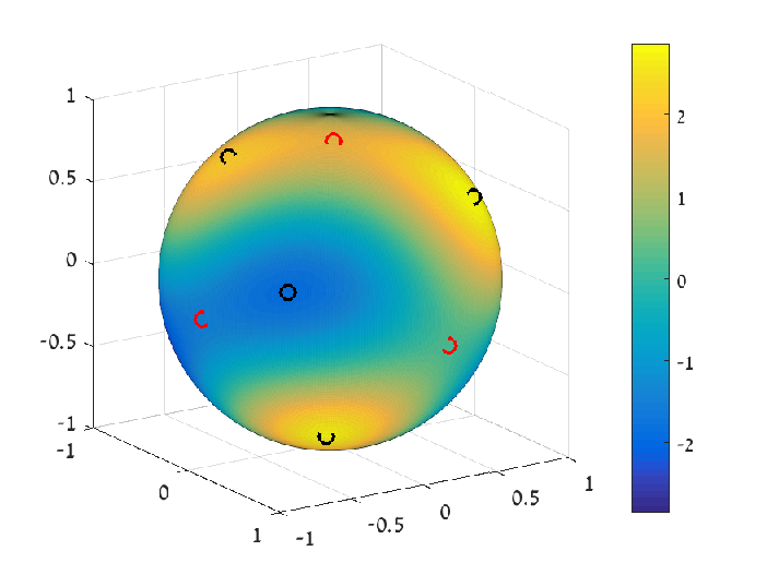
As an example, the left panel of Figure 1 shows the value of $\mu(\bm{x})$ over the unit sphere for a $3\times 3\times 3$ symmetric tensor with $7$ real eigenvectors. Three eigenvectors, depicted in red, are power-unstable, while the remaining four, depicted in black, are power-stable. The right panel of the same figure shows the results of the adaptive shifted-HOPM. The color indicates the eigenvector to which the method converged, starting from various locations on the unit sphere. The figure shows clear convergence regions around $3$ of the power-stable eigenpairs. The region around the fourth power-stable eigenpair appears on the back side of the sphere. In agreement with theory, the adaptive HOPM did not converge to any of the three power-unstable eigenpairs.

Newton-based methods for the tensor eigen-problem

Given the limitations of the aforementioned methods, our goal is to derive a fast iterative algorithm that under mild assumptions is able to converge to all real eigenpairs of a symmetric tensor. To this end, we develop a Newton-based method.

4.1 Newton correction method

Several variants of Newton’s method were derived for the symmetric matrix eigen-problem, see for example [30, Chapter 6]. Here we derive a Newton-based method for computing the eigenpairs of symmetric tensors. Recently, [12] considered a similar approach for finding some nonnegative eigenpairs of a nonnegative tensor.

Let $(\bm{x}^{\ast},\lambda^{\ast})$ be an eigenpair of a symmetric tensor $\mathcal{T}$ of order $m$ and dimensionality $n$ . Given an approximation $\bm{x}$ to $\bm{x}^{\ast}$ , our goal is to obtain an improved approximation $\bm{x}^{\prime}$ (see Figure 3, left). Denote the exact unknown correction by $\bm{y}^{*}=\bm{x}^{\ast}-\bm{x}$ and recall $\mu(\bm{x})=\mathcal{T}(\bm{x},\ldots,\bm{x})$ . Since $\bm{x}^{\ast}=\bm{x}+\bm{y}^{*}$ and $\lambda^{\ast}=\mu(\bm{x}^{\ast})=\mu(\bm{x}+\bm{y}^{*})$ , the eigen-problem in (1) can be written as

\displaystyle\mathcal{T}(I,\bm{x}+\bm{y}^{*},\ldots,\bm{x}+\bm{y}^{*})=\mu(\bm{x}+\bm{y}^{*})\cdot(\bm{x}+\bm{y}^{*}).

(10)

Recalling the Hessian matrix $H(\bm{x})$ in (5), we define the matrix $A(\bm{x})\in\mathbb{R}^{n\times n}$ by

A(\bm{x})=H(\bm{x})-m\bm{x}\mathcal{T}(I,\bm{x},\ldots,\bm{x})^{T}.

(11)

Setting apart the terms that are linear in $\bm{y}^{*}$ , Eq. (10) takes the form

\displaystyle A(\bm{x})\bm{y}^{*}=-\bm{g}(\bm{x})+\Delta(\bm{x},\bm{y}^{*}),

(12)

where $\bm{g}(\bm{x})$ is given in (4). Here, $\Delta(\bm{x},\bm{y}^{*})$ accounts for all high order terms in $\bm{y}^{*}$ ,

	$\displaystyle\Delta(\bm{x},\bm{y}^{*})$	$\displaystyle=\sum_{i=2}^{m}\binom{m}{i}\mathcal{T}(\underbrace{\bm{x},\ldots,\bm{x}}_{m-i},\underbrace{\bm{y}^{},\ldots,\bm{y}^{}}_{i})\bm{x}+\sum_{i=1}^{m}\binom{m}{i}\mathcal{T}(\underbrace{\bm{x},\ldots,\bm{x}}_{m-i},\underbrace{\bm{y}^{},\ldots,\bm{y}^{}}_{i})\bm{y}^{*}$
		$\displaystyle-\sum_{i=2}^{m-1}\binom{m-1}{i}\mathcal{T}(I,\underbrace{\bm{x},\ldots,\bm{x}}_{m-i-1},\underbrace{\bm{y}^{},\ldots,\bm{y}^{}}_{i}).$		(13)

Algorithm 1 Newton correction method

1: Input: tensor

\mathcal{T}\in\mathbb{R}^{n\times\dots\times n}

, tolerance parameter

\delta>0

2: Initialization: Randomly choose

\bm{x}_{(0)}\in S_{n-1}

3: Set

k=0

and

\lambda_{(0)}=\mu(\bm{x}_{(0)})

4: while

\|\bm{x}_{(k)}-\bm{x}_{(k-1)}\|>\delta

5: Compute

\bm{y}_{(k)}=-A(\bm{x}_{(k)})^{-1}\bm{g}(\bm{x}_{(k)})

6: Set

\bm{x}_{(k+1)}=(\bm{x}_{(k)}+\bm{y}_{(k)})/{\|\bm{x}_{(k)}+\bm{y}_{(k)}\|}

7: Set

\lambda_{(k+1)}=\mu(\bm{x}_{(k+1)})

k\leftarrow k+1

9: end while

10: return

(\bm{x}_{(k)},\lambda_{(k)})

By definition, the solution $\bm{y}^{*}$ to (12) satisfies $\bm{x}+\bm{y}^{*}=\bm{x}^{\ast}$ . However, solving (12) exactly for $\bm{y}^{*}$ is as difficult as finding the eigenpair $(\bm{x}^{\ast},\lambda^{\ast}$ ) of the tensor $\mathcal{T}$ we started from. Instead, we devise an iterative Newton correction method (NCM) that solves (12) only approximately. Given the approximation $\bm{x}_{(k)}$ of $\bm{x}^{\ast}$ at the $k^{\text{th}}$ iteration, NCM computes a new approximation $\bm{x}_{(k+1)}$ by neglecting the high order terms $\Delta(\bm{x},\bm{y}^{*})$ in (12). This amounts to solving the system of $n$ linear equations

A(\bm{x}_{(k)})\bm{y}_{(k)}=-\bm{g}(\bm{x}_{(k)}).

(14)

Assuming $A(\bm{x}_{(k)})$ is invertible, the unique solution to (14) is given by

\displaystyle\bm{y}_{(k)}=-A(\bm{x}_{(k)})^{-1}\bm{g}(\bm{x}_{(k)}).

(15)

The new approximation $\bm{x}_{(k+1)}$ for $\bm{x}^{\ast}$ is then

\displaystyle\bm{x}_{(k+1)}=\frac{\bm{x}_{(k)}+\bm{y}_{(k)}}{{\|\bm{x}_{(k)}+\bm{y}_{(k)}\|}}.

(16)

Given an initial guess $\bm{x}_{(0)}\in S_{n-1}$ , NCM iterates steps (15) and (16). Once a stopping condition is met, the pair $(\bm{x}_{(k)},\mu(\bm{x}_{(k)}))$ is returned; see Algorithm 1.

The left panel of Figure 2 shows the convergence regions of NCM for the eigenpairs of the same tensor as in Figure 1. In this case, all eigenpairs are attracting points of NCM and can thus be found by running Algorithm 1 multiple times with different (random) initial guesses.

Convergence guarantees

Two questions regarding NCM are (i) to which eigenpairs of $\mathcal{T}$ the method can converge to? and (ii) what is the convergence rate? To answer these questions we recall the definition of the Hessian matrix in (5). Given an eigenpair $(\bm{x}^{\ast},\lambda^{\ast})$ , its corresponding Hessian matrix is

H(\bm{x}^{\ast})=(m-1)\mathcal{T}(I,I,\bm{x}^{\ast},\ldots,\bm{x}^{\ast})-\lambda^{\ast}I.

Note that $H(\bm{x}^{\ast})$ is symmetric and has $\bm{x}^{\ast}$ as an eigenvector with eigenvalue $(m-2)\lambda^{\ast}$ . Denote by $\mu_{1}^{\ast},\ldots,\mu_{n-1}^{\ast}$ the other $n-1$ eigenvalues of $H(\bm{x}^{\ast})$ . By definition, these are the eigenvalues of the projected Hessian $H_{p}(\bm{x}^{\ast})$ in (9).

Definition 2

For $\gamma>0$ , an eigenpair $(\bm{x}^{\ast},\lambda^{\ast})$ is $\gamma$ -Newton-stable if all eigenvalues of $H_{p}(\bm{x}^{\ast})$ in absolute value are at least $\gamma$ , namely, $\min_{i}|\mu_{i}^{*}|\geq\gamma$ .

Note that $H_{p}(\bm{x}^{\ast})$ is full rank iff $\bm{x}^{\ast}$ is $\gamma$ -Newton-stable for some $\gamma>0$ . Similarly, $H(\bm{x}^{\ast})$ is full rank iff $\bm{x}^{\ast}$ is $\gamma$ -Newton-stable for some $\gamma>0$ and $\lambda^{\ast}\neq 0$ . We have the following convergence guarantee for NCM. The proof is given in Appendix A.

Theorem 1

Let $(\bm{x}^{\ast},\lambda^{\ast})$ be an eigenpair of a symmetric tensor $\mathcal{T}$ . Suppose that $(\bm{x}^{\ast},\lambda^{\ast})$ is $\gamma$ -Newton-stable and that $\lambda^{\ast}\neq 0$ . Then there exists an $\varepsilon=\varepsilon(\gamma,\lambda^{\ast})>0$ such that for any $\bm{x}_{(0)}$ that satisfies ${\|\bm{x}_{(0)}-\bm{x}^{\ast}\|}<\varepsilon$ , the sequence $\bm{x}_{(0)},\bm{x}_{(1)},\dots$ , computed by Algorithm 1 converges to $\bm{x}^{\ast}$ at a quadratic rate.

4.2 Orthogonal Newton correction method

Figure 3: Illustration of one iteration of NCM (left) and O–NCM (right).

As discussed above, the NCM method may not converge to an eigenvector with eigenvalue $\lambda^{\ast}=0$ . To remove this limitation, we now develop an orthogonal NCM variant. Given an approximation $\bm{x}\in S_{n-1}$ of $\bm{x}^{\ast}$ , we first decompose it into its projection onto $\bm{x}^{\ast}$ and a residual (see Figure 3, right),

\bm{x}=\alpha\bm{x}^{\ast}-\bm{u}^{*},

(17)

where $\alpha=\bm{x}^{T}\bm{x}^{\ast}$ and $\bm{u}^{*}=\alpha\bm{x}^{\ast}-\bm{x}$ is the residual. Since $\bm{x}^{\ast}$ and $\bm{u}^{*}$ are orthogonal and $\bm{x}\in S_{n-1}$ , ${\|\bm{x}\|}^{2}=\alpha^{2}+{\|\bm{u}^{*}\|}^{2}=1$ . For reasons to become clear shortly, we also introduce a correction $\beta^{*}\equiv\beta^{*}(\bm{x},\bm{x}^{\ast})$ to the eigenvalue $\lambda^{\ast}$ , defined as

\displaystyle\beta^{*}=\alpha^{m-2}\lambda^{\ast}-\mathcal{T}(\bm{x},\dots,\bm{x})=\alpha^{m-2}\lambda^{\ast}-\mu(\bm{x}).

(18)

When $\bm{x}=\bm{x}^{\ast}$ , we have $\bm{u}^{*}=0$ , $\alpha=1$ and $\beta^{*}=0$ . Since $(\bm{x}^{\ast},\lambda^{\ast})$ is an eigenpair,

\mathcal{T}(I,\alpha\bm{x}^{\ast},\ldots,\alpha\bm{x}^{\ast})=\alpha^{m-1}\lambda^{\ast}\bm{x}^{\ast}.

Inserting $\bm{x}^{\ast}=\frac{1}{\alpha}(\bm{x}+\bm{u}^{*})$ and $\beta^{*}$ into the above equation gives

\displaystyle\begin{split}\mathcal{T}(I,\bm{x}+\bm{u}^{*},\ldots,\bm{x}+\bm{u}^{*})=(\mu(\bm{x})+\beta^{*})\cdot(\bm{x}+\bm{u}^{*}).\end{split}

(19)

We set apart the terms that are linear in $\bm{u}^{*}$ and $\beta^{*}$ to obtain

H(\bm{x})\bm{u}^{*}-\beta^{*}\bm{x}=-\bm{g}(\bm{x})+\tilde{\Delta}(\bm{x},\bm{u}^{*},\beta^{*}),

(20)

where $\bm{g}$ and $H$ were defined in (4) and (5) respectively and $\tilde{\Delta}(\bm{x},\bm{u}^{*},\beta^{*})$ includes all the remaining higher order terms in $(\bm{u}^{*},\beta^{*})$ ,

\displaystyle\tilde{\Delta}(\bm{x},\bm{u}^{*},\beta^{*})=\beta^{*}\bm{u}^{*}-\sum_{i=2}^{m-1}\tbinom{m-1}{i}\mathcal{T}(I,\underbrace{\bm{x},\ldots,\bm{x}}_{m-i-1},\underbrace{\bm{u}^{*},\ldots,\bm{u}^{*}}_{i}).

(21)

Combining (20) with the orthogonality condition, $(\bm{x}^{\ast})^{T}\bm{u}^{*}\propto(\bm{x}+\bm{u}^{*})^{T}\bm{u}^{*}=0$ , gives the following set of non-linear equations in $(\bm{u}^{\ast},\beta^{*})$ ,

\displaystyle{\begin{pmatrix}H(\bm{x})&-\bm{x}\\ \bm{x}^{T}&0\\ \end{pmatrix}\begin{pmatrix}\bm{u}^{*}\\ \beta^{*}\end{pmatrix}}=-{\begin{pmatrix}\bm{g}(\bm{x})\\ 0\end{pmatrix}+\begin{pmatrix}\tilde{\Delta}(\bm{x},\bm{u}^{*},\beta^{*})\\ -{\|\bm{u}^{*}\|}^{2}\end{pmatrix}}.

(22)

By construction, the solution $(\bm{u}^{\ast},\beta^{*})$ to (22) satisfies $(\bm{x}+\bm{u}^{\ast})/{\|\bm{x}+\bm{u}^{\ast}\|}=\bm{x}^{\ast}$ . Similarly to the NCM, we neglect the high order terms in the right hand side of (22) and solve the system of linear equations in the $n+1$ unknowns $(\bm{u},\beta)$ ,

\begin{pmatrix}H(\bm{x})&-\bm{x}\\ \bm{x}^{T}&0\\ \end{pmatrix}\begin{pmatrix}\bm{u}\\ \beta\end{pmatrix}=-\begin{pmatrix}\bm{g}(\bm{x})\\ 0\end{pmatrix}.

(23)

Algorithm 2 Orthogonal Newton correction method

1: Input: tensor

\mathcal{T}

, threshold

\delta

2: Initialization: Randomly choose

\bm{x}_{(0)}\in S_{n-1}

3: Set

k=0

and

\lambda_{(0)}=\mu(\bm{x}_{(0)})

4: while

\|\bm{x}_{(k)}-\bm{x}_{(k-1)}\|>\delta

5: Compute

\bm{u}_{(k)}=-U_{\bm{x}_{(k)}}H_{p}(\bm{x}_{(k)})^{-1}U_{\bm{x}_{(k)}}^{T}\bm{\bm{g}}(\bm{x}_{(k)})

6: Set

\bm{x}_{(k+1)}=(\bm{x}_{(k)}+\bm{u}_{(k)})/{\|\bm{x}_{(k)}+\bm{u}_{(k)}\|}

7: Set

\lambda_{(k+1)}=\mu(\bm{x}_{(k+1)})

k\leftarrow k+1

9: end while

10: return

(\bm{x}_{(k)},\lambda_{(k)})

Due to the extra variable $\beta$ , (23) seems to be of dimension $n+1$ , as opposed to the $n$ dimensional system in (14). However, as we now show, the system in (23) can be equivalently solved in the $n-1$ dimensional subspace orthogonal to $\bm{x}$ . More precisely, let $P_{\bm{x}}^{\perp}=(I-\bm{x}\bm{x}^{T})$ be the projection matrix into the subspace orthogonal to $\bm{x}$ and let $U_{\bm{x}}\in\mathbb{R}^{n\times(n-1)}$ have orthonormal columns such that $P_{\bm{x}}^{\perp}=U_{\bm{x}}U_{\bm{x}}^{T}$ . Recall the projected Hessian matrix $H_{p}(\bm{x})=U_{\bm{x}}^{T}H(\bm{x})U_{\bm{x}}$ in (9). The following lemma is an adaptation of [30, Theorem 6.2.2] to our setting. Its proof is given in Appendix B.

Lemma 1

A vector $\bm{u}\in\mathbb{R}^{n}$ satisfies (23) if and only if $\bm{z}\in\mathbb{R}^{n-1}$ satisfies

\displaystyle H_{p}(\bm{x})\bm{z}=-U_{\bm{x}}^{T}\bm{g}(\bm{x})\quad\text{and}\quad\bm{u}=U_{\bm{x}}\bm{z}.

(24)

Assuming $H_{p}(\bm{x})$ is invertible, the solution to (24) is $\bm{u}=-U_{\bm{x}}H_{p}(\bm{x})^{-1}U_{\bm{x}}^{T}\bm{g}(\bm{x}).$ So given the $k^{\text{th}}$ approximation $\bm{x}_{(k)}$ to $\bm{x}^{\ast}$ , O–NCM computes

\bm{u}_{(k)}=-U_{\bm{x}_{(k)}}H_{p}(\bm{x}_{(k)})^{-1}U_{\bm{x}_{(k)}}^{T}\bm{g}(\bm{x}_{(k)})

(25)

and the new approximation is $\bm{x}_{(k+1)}=(\bm{x}_{(k)}+\bm{u}_{(k)})/{\|\bm{x}_{(k)}+\bm{u}_{(k)}\|}$ . Given an initial $\bm{x}_{(0)}$ , O–NCM iterates these steps until a stopping condition is met; see Algorithm 2.

The right panel of Figure 2 shows the convergence regions of O–NCM for the various eigenpairs of the same tensor in Figure 1. Similarly to NCM, in this case, all eigenpairs are attracting points of O–NCM, but with slightly different regions.

Convergence guarantees

We have the following convergence guarantee for O–NCM. It is similar to that of NCM in Theorem 1, but with the condition $\lambda^{*}\neq 0$ removed. The proof is given in Appendix C.

Theorem 2

Let $(\bm{x}^{\ast},\lambda^{\ast})$ be a $\gamma$ -Newton-stable eigenpair of a symmetric tensor $\mathcal{T}$ . There exists an $\varepsilon=\varepsilon(\gamma)>0$ such that for any $\bm{x}_{(0)}\in S_{n-1}$ that satisfies ${\|\bm{x}_{(0)}-\bm{x}^{\ast}\|}<\varepsilon$ , the sequence $\bm{x}_{(0)},\bm{x}_{(1)},\dots$ , computed by Algorithm 2 converges to $\bm{x}^{\ast}$ at a quadratic rate.

Remark 1

Recall that any eigenpair $(\bm{x}^{\ast},\lambda^{\ast})$ to which the shifted-HOPM method converges to has a Hessian matrix which is either positive definite or negative definite. In either case, this Hessian matrix has full rank, and thus by Theorem 2, is a stable fixed point of O–NCM. In other words, O–NCM typically converges to many more tensor eigenpairs than the shifted power method. However, the adaptive shifted-HOPM is guaranteed to converge from any initial point, whereas no such global convergence guarantee is currently available for the Newton-based methods.

Convergence to eigenpairs with a rank deficient Hessian

The sufficient condition in Theorem 2 for O–NCM to converge to an eigenpair $(\bm{x}^{\ast},\lambda^{\ast})$ rests on the smallest absolute eigenvalue of the projected Hessian matrix $H_{p}(\bm{x}^{\ast})$ . In particular, if the eigenpair is $\gamma$ -Newton-stable for some $\gamma>0$ , an attraction neighborhood around $\bm{x}^{\ast}$ exists. We now illustrate that this sufficient condition for convergence is by no means necessary. To this end, we analyze a simple example. Denote $\bm{1}=(1,\ldots,1)^{T}\in\mathbb{R}^{n}$ . For any $\omega\in\mathbb{R}$ , define the following cubic $n$ -dimensional symmetric tensor,

\mathcal{T}_{\omega}=\sum_{i=1}^{n}\bm{e}_{i}\otimes\bm{e}_{i}\otimes\bm{e}_{i}+\omega(\bm{1}\otimes\bm{1}\otimes\bm{1}).

(26)

When $\omega=0$ , $\mathcal{T}_{\omega}$ is orthogonal, having the maximally possible number of $2^{n}-1$ real eigenpairs. All these are Newton-stable and among them are the $n$ power-stable eigenpairs $\{(\bm{e}_{i},1)\}_{i=1}^{n}$ . Assume $n$ is odd and denote $l=\lfloor n/2\rfloor$ . Let $N(\omega)$ be the number of real eigenpairs of $\mathcal{T}_{\omega}$ . The following proposition is proved in Appendix D.

Proposition 1

Define $l$ thresholds, $\omega_{i}=\frac{1}{4(l-i)(n-l+i)}>0$ , $i\in\{0,\ldots,l-1\}$ .

(i)

The number $N(\omega)$ of real eigenpairs of $\mathcal{T}_{\omega}$ of Eq. (26) is

N(\omega)=\begin{cases}2^{n}-1&\omega<\omega_{0}\\ 1+2\sum_{j=1}^{l-i-1}\binom{n}{j}+\binom{n}{l-i}&\omega=\omega_{i}\\ 1+\sum_{j=1}^{l-i-1}\binom{n}{j}&\omega_{i}<\omega<\omega_{i+1}\\ 1&\omega>\omega_{l-1}.\end{cases}

(ii)

For $\omega_{i}\in\{\omega_{0},\dots,\omega_{l-1}\}$ , $\binom{n}{l-i}$ out of the $N(\omega_{i})$ real eigenpairs of $\mathcal{T}(\omega_{i})$ are not Newton-stable.

We illustrate the above properties for $\mathcal{T}_{\omega}$ with $n=5$ . In this case, $l=\lfloor n/2\rfloor=2$ and there are two thresholds, $\omega_{0}=\frac{1}{4\cdot 2\cdot 3}\approx 0.0417$ and $\omega_{1}=\frac{1}{4\cdot 1\cdot 4}=0.0625$ . Figure 4 shows the number $N(\omega)$ of real eigenpairs (left), and the different eigenvalues of $\mathcal{T}_{\omega}$ (right) as computed by O–NCM. As expected, at $\omega_{0}$ and $\omega_{1}$ , the number of real eigenvalues decreases.

Next, we examine the convergence of O–NCM on $\mathcal{T}_{\omega=\omega_{0}}$ with $n=3$ . According to Proposition 1, $\omega_{0}=0.125$ , and the number of real eigenpairs is $N(\omega_{0})=1+\binom{3}{1}=4$ , three of which are not Newton-stable. Figure 5 shows the attraction regions around two of the eigevectors of $\mathcal{T}_{\omega_{0}}$ , as well as the full unit sphere. On the left, the eigenvector is Newton-stable. As expected, O–NCM converged to this eigenvector from any point in its neighborhood. In contrast, the eigenvector on the right is not Newton-stable. In this case, there is a positive probability of converging to a different eigenvector even when the initial guess is arbitrary close. Nonetheless, O–NCM converged to this eigenvector from some directions, even though the sufficient condition in Theorem 2 does not hold.

In this example, all eigenpairs of $\mathcal{T}_{\omega}$ are isolated, namely each one of them is the unique eigenpair in a small neighborhood around it. In addition, the eigenvectors which are not Newton-stable have a projected Hessian matrix that is rank deficient but non-zero. In Appendix E, we illustrate the behavior of O–NCM near eigenvectors that are either non-isolated, or have a projected Hessian matrix equals to zero. In these cases, O–NCM may not converge.

Simulation results

In this section we study numerically the performance of NCM and O–NCM for computing the real eigenpairs of symmetric tensors, as compared to the homotopy method [7] and the adaptive shifted-HOPM [19].¹¹ 1 Matlab code for the NCM methods can be found at https://github.com/arJaffe/NCM, for the homotopy method at http://users.math.msu.edu/users/chenlipi/TenEig.html, and for the shifted HOPM at http://www.sandia.gov/~tgkolda/TensorToolbox/index-2.6.html. In the experiments we consider random Gaussian symmetric tensors, whose entries are all i.i.d. $\mathcal{N}(0,1)$ up to the symmetry constraints. All experiments were done on a PC with an Intel i-3820 $3.6\text{GHz}$ processor, $16\text{GB}$ RAM and MATLAB version R2016a.

Finding all real eigenpairs

We examine the time needed to compute all eigenpairs for random tensors of order $m=4$ and various dimensions $n$ . Similar results are obtained for other values of $m$ . For each tensor, we first ran the homotopy method to obtain all its eigenpairs. Next, we ran NCM and O–NCM, initialized repeatedly with random points on the unit sphere, until all eigenpairs were found. Note that without running the homotopy method first, we would have no criterion to decide whether we actually found all tensor’s eigenpairs. The process was sequential, where a new run was initialized only after the previous one ended. This process, however, can be easily parallelized. We stopped the NCM iterations when $\|\bm{x}_{(k)}-\bm{x}_{(k-1)}\|<\delta=10^{-10}$ or if a maximal number of $k=k_{\max}=200$ iterations was reached. In the latter case we declared that NCM failed to converge. For both NCM and O–NCM, and for all tensor dimensions we considered, only $\approx 0.2\%$ of all random initializations failed to converge within the maximal number of iterations.

Figure 6 (left) shows the number of real eigenpairs as averaged over 10 independent tensors for each value of $n$ . Figure 6 (right) shows on a logarithmic scale the average time it took to compute all real eigenpairs via the homotopy, NCM and O–NCM, for the same tensors. These results show that both NCM and O–NCM recovered all eigenpairs faster than the homotopy method by approximately two orders of magnitude. Moreover, O–NCM did so much faster than NCM.

Small eigenvalues

To understand the gap in the runtime of NCM and O–NCM shown in Figure 6, we next examine the dependence of both methods on the eigenpair to which they converge. As suggested by Theorems 1 and 2, we expect O–NCM to have larger attraction regions for small eigenvalues as compared to NCM. Figure 7 (left) shows on a log-log scale the relative number of times the two methods converged to each eigenvalue as a function of its absolute value for a typical random tensor of order $m=4$ and dimension $n=8$ . These counts correspond to a total of $10^{6}$ random initializations uniformly distributed on the unit sphere. As one can see, the probability for NCM to converge to an eigenpair decreases sharply when its eigenvalue becomes small, while for O–NCM this probability seems to be independent of $|\lambda|$ . This difference is the source of the gap in the runtime of the two methods for finding all eigenpairs. For completeness, the eigenvalues found by the adaptive S-HOPM are also presented.

Convergence rates

Figure 7 (right) shows the median runtime till convergence of the NCM and the shifted HOPM. The stopping condition for all methods was set to $\|\bm{x}_{(k)}-\bm{x}_{(k+1)}\|<\delta=10^{-10}$ . The experiment was done on $100$ random tensors of fourth order with various dimensions. For each tensor, we initialized all methods with $100$ random starting points. To avoid the influence of any particular implementation, we normalized the results with the runtime of both methods for $n=3$ . As illustrated in Fig. 7, the runtime increase of the NCM or O–NCM is significantly slower than the corresponding increase in the adaptive shifted-HOPM. However, each NCM/O–NCM iteration may be slower, as it requires matrix inversion.

Discussion and summary

In this paper we developed and analyzed a Newton-based iterative approach to compute real eigenpairs of symmetric tensors. We now briefly discuss three important issues: its runtime, its ability to find all tensor eigenpairs, and its optimization point of view.

Runtime

The computational complexity of each NCM or O–NCM iteration is dominated by two operations: computing the Hessian matrix in $\mathcal{O}(n^{m})$ time and solving a system of $n$ linear equations in $\mathcal{O}(n^{3})$ time. The latter step may be significantly sped up by applying various preconditioning techniques, as done in other iterative methods that solve systems of linear equations [10]. For sparse tensors, the computation of the Hessian can be accelerated as well, see [29].

Optimization point of view

Following a constructive comment by one of the referees, we note that NCM can be seen as an adaptation of the Gauss–Newton method [3]. Recall that $\bm{g}(\bm{x})=\mathcal{T}(I,\bm{x},\dots,\bm{x})-\mu(\bm{x})\bm{x}=\bm{0}$ if and only if $\bm{x}^{\ast}\in S_{n-1}$ is an eigenvector of $\mathcal{T}$ , with a corresponding eigenvalue $\lambda^{*}=\mu(\bm{x}^{\ast})$ . Hence, our goal is to find the global minima of the realizable nonlinear least-squares problem

\displaystyle\min_{\bm{x}\in S_{n-1}}\tfrac{1}{2}{\|\bm{g}(\bm{x})\|}^{2}.

(27)

Given the current estimate $\bm{x}_{(k)}\in S_{n-1}$ , Gauss–Newton first linearizes $\bm{g}(\bm{x})$ at $\bm{x}_{(k)}$ ,

\displaystyle\bm{g}(\bm{x})\approx\bm{g}(\bm{x}_{(k)})+A(\bm{x}_{(k)})(\bm{x}-\bm{x}_{(k)})=\bm{g}(\bm{x}_{(k)})+A(\bm{x}_{(k)})\bm{y},

where $[A(\bm{x})]_{ij}=\partial g_{i}(\bm{x})/\partial x_{j}$ is the $n\times n$ Jacobian matrix of $\bm{g}(\bm{x})$ , given in (11). Then, instead of (27), the following approximate linear least-squares problem is solved,

\displaystyle\bm{y}_{(k)}=\argmin_{\bm{y}\in\mathbb{R}^{n}}\tfrac{1}{2}{\|\bm{g}(\bm{x}_{(k)})+A(\bm{x}_{(k)})\bm{y}\|}^{2},

which is exactly the NCM correction in (14).

Besides NCM, other nonlinear optimization methods can be used to solve (27), such as the Levenberg-Marquardt algorithm [23] and other trust-region and line search algorithms. These methods, among other things, introduce an additional regularization term to better control the direction in which the method proceeds at each iteration, similarly to the role played by the (adaptive) shifted-HOPM as compared to HOPM. Specifically, instead of (14), one solves the following linear system with an appropriate regularization matrix $B_{k}\in\mathbb{R}^{n\times n}$ ,

\displaystyle(A(\bm{x}_{(k)})^{T}A(\bm{x}_{(k)})+B_{k})\bm{y}=-A(\bm{x}_{(k)})^{T}\bm{g}(\bm{x}_{(k)}).

While NCM currently has no global convergence guarantees, an appropriate (adaptive) choice of $B_{k}$ can lead to global convergence guarantees, including to eigenvectors having a zero Hessian. Further studying the role of regularization for the tensor eigen-problem is an interesting direction for future research.

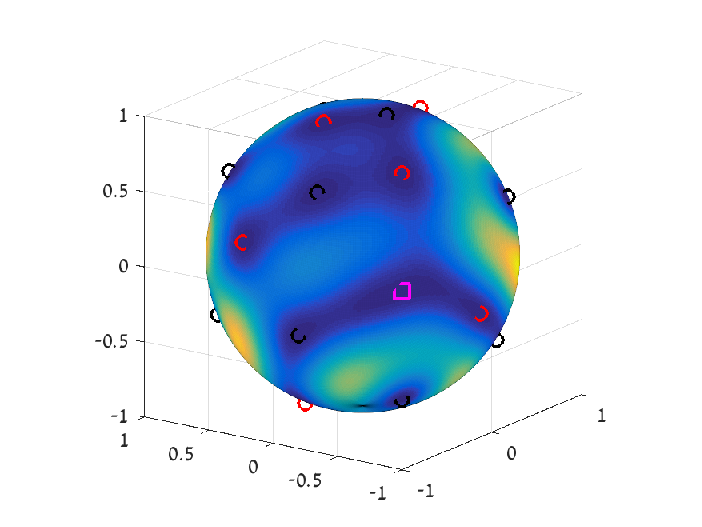
However, in addition to the global minima, $f(\bm{x})\equiv\frac{1}{2}{\|\bm{g}(\bm{x})\|}^{2}$ may have local minima which should be avoided. Interestingly, NCM elegantly avoids such local minima as the following example illustrates. In Figure 8 (left), we plot $f(\bm{x})$ as a function of $\bm{x}\in S_{2}$ for the $3\times 3\times 3\times 3$ symmetric tensor of Example 1 in [17]. Its eigenvectors are depicted by circles while a local minimum $\bm{x}_{\text{loc}}$ of $f$ is depicted by a square symbol. In Figure 8 (right) we show the attraction regions for NCM starting from various locations on $S_{n-1}$ . As one can see, NCM does not converge to $\bm{x}_{\text{loc}}$ and in fact is highly unstable around this point; close initial points in this neighborhood may converge to arbitrarily far eigenvectors.

To see why this is so, note that since $\bm{x}_{\text{loc}}$ is a local minimum, for an initial point $\bm{x}_{(0)}$ near $\bm{x}_{\text{loc}}$ , NCM may get closer and closer to $\bm{x}_{\text{loc}}$ at the first few iterations. However, the facts that $\bm{g}(\bm{x}_{\text{loc}})$ is bounded away from $\bm{0}$ and $\nabla f(\bm{x}_{\text{loc}})=A(\bm{x}_{\text{loc}})^{T}\bm{g}(\bm{x}_{\text{loc}})=\bm{0}$ implies that $\bm{g}(\bm{x}_{\text{loc}})$ is in the null space of $A(\bm{x}_{\text{loc}})^{T}$ . As $\bm{x}_{(k)}$ gets closer to $\bm{x}_{\text{loc}}$ , $A(\bm{x}_{(k)})$ becomes close to singular. The result is an overshoot, a sharp increase in ${\|\bm{y}_{(k)}\|}={\|A(\bm{x}_{(k)})^{-1}\bm{g}(\bm{x}_{(k)})\|}$ , taking $\bm{x}_{(k+1)}$ far away from $\bm{x}_{(k)}$ and $\bm{x}_{\text{loc}}$ .

Finding all eigenpairs of generic tensors

According to our theoretical analysis, NCM and O–NCM converge to eigenpairs whose Hessian matrix is full rank. An interesting question is whether these methods can thus converge to all real eigenpairs of a generic symmetric tensor [5]. Interpreting generic in the sense of algebraic geometry, an adaptation of [5, Theorem 1.2] to the symmetric tensor case implies the following (proof omitted).

Proposition 2

All real eigenpairs of a generic symmetric tensor are Newton-stable.

Hence, Theorems 1 and 2 imply that NCM and O–NCM are guaranteed to find all eigenpairs of a generic symmetric tensor given a sufficiently large number of random initializations.

Acknowledgments

We thank Lek–Heng Lim, Meirav Galun and Haim Avron for interesting discussions.

Appendix A Convergence of NCM

To prove Theorem 1 we shall make use of the following auxiliary lemma.

Lemma 2

Consider one update step of Algorithm 1, as in Equation (16), starting from an initial $\bm{x}\in S_{n-1}$ and ending with $\bm{x}^{\prime}=(\bm{x}+\bm{y})/{\|\bm{x}+\bm{y}\|}\in S_{n-1}$ . Let $\bm{y}^{*}=\bm{x}^{\ast}-\bm{x}$ . If ${\|\bm{y}-\bm{y}^{*}\|}\leq 1/2$ , then

\displaystyle{\|\bm{x}^{\ast}-\bm{x}^{\prime}\|}\leq\frac{2{\|\bm{y}^{*}-\bm{y}\|}}{1-{{\|\bm{y}^{*}-\bm{y}\|}}}.

(28)

Proof 1

By definition,

	$\displaystyle{\\|\bm{x}^{\ast}-\bm{x}^{\prime}\\|}$	$\displaystyle=$	$\displaystyle\left\\|\bm{x}^{\ast}-\frac{\bm{x}+\bm{y}}{{\\|\bm{x}+\bm{y}\\|}}\right\\|=\left\\|\bm{x}^{\ast}-\frac{\bm{x}^{\ast}-\bm{y}^{}+\bm{y}}{{\\|\bm{x}^{\ast}-\bm{y}^{}+\bm{y}\\|}}\right\\|$		(29)
		$\displaystyle=$	$\displaystyle\left\\|{\bm{x}^{\ast}\left(1-\frac{1}{{\\|\bm{x}^{\ast}-\bm{y}^{}+\bm{y}\\|}}\right)+\frac{\bm{y}^{}-\bm{y}}{{\\|\bm{x}^{\ast}-\bm{y}^{*}+\bm{y}\\|}}}\right\\|.$		(29)

Since ${\|\bm{x}^{\ast}\|}=1$ , by the triangle inequality,

\displaystyle 1-{\|\bm{y}^{*}-\bm{y}\|}\leq{\|\bm{x}^{\ast}-\bm{y}^{*}+\bm{y}\|}\leq 1+{\|\bm{y}^{*}-\bm{y}\|}.

Applying the triangle inequality to (29), combined with the assumption ${\|\bm{y}^{*}-\bm{y}\|}\leq 1/2$ ,

	$\displaystyle{\\|\bm{x}^{\ast}-\bm{x}^{\prime}\\|}$	$\displaystyle\leq$	$\displaystyle\left\|1-\frac{1}{{\\|\bm{x}^{\ast}-\bm{y}^{}+\bm{y}\\|}}\right\|+\frac{{\\|\bm{y}^{}-\bm{y}\\|}}{{\\|\bm{x}^{\ast}-\bm{y}^{*}+\bm{y}\\|}}$
		$\displaystyle\leq$	$\displaystyle\left(\frac{1}{1-{\\|\bm{y}^{}-\bm{y}\\|}}-1\right)+\frac{{\\|\bm{y}^{}-\bm{y}\\|}}{1-{\\|\bm{y}^{}-\bm{y}\\|}}=\frac{2{\\|\bm{y}^{}-\bm{y}\\|}}{1-{{\\|\bm{y}^{*}-\bm{y}\\|}}},$

hence concluding the proof.

Proof 2 (Proof of Theorem 1)

To prove quadratic convergence it suffices to show that there exists an $\varepsilon>0$ and a constant $C>0$ such that from any initial point $\bm{x}_{(0)}$ that satisfies ${\|\bm{x}_{(0)}-\bm{x}^{\ast}\|}<\varepsilon$ ,

\displaystyle e_{k}=\frac{{\|\bm{x}^{\ast}-\bm{x}_{(k+1)}\|}}{{\|\bm{x}^{\ast}-\bm{x}_{(k)}\|}^{2}}<C,\quad\forall k\geq 0.

We start by analyzing $e_{k}$ at the first iteration $k=0$ . Let $\bm{y}_{(0)}$ be the approximate correction of $\bm{y}^{*}=\bm{x}^{\ast}-\bm{x}_{(0)}$ , given by the solution of (14). The new approximation of $\bm{x}^{\ast}$ , given by Eq. (16), is $\bm{x}_{(1)}=(\bm{x}_{(0)}+\bm{y}_{(0)})/{\|\bm{x}_{(0)}+\bm{y}_{(0)}\|}$ . Assume for the moment that the initial guess $\bm{x}_{(0)}$ is sufficiently close to $\bm{x}^{\ast}$ so that ${\|\bm{y}^{*}-\bm{y}_{(0)}\|}<1/2$ . Then, by Lemma 2,

\displaystyle{\|\bm{x}^{\ast}-\bm{x}_{(1)}\|}\leq\frac{2{\|\bm{y}^{*}-\bm{y}_{(0)}\|}}{1-{{\|\bm{y}^{*}-\bm{y}_{(0)}\|}}}.

(30)

Hence, it suffices to bound ${\|\bm{y}^{*}-\bm{y}_{(0)}\|}$ . To this end, we view the exact system of non-linear equations (12), whose solution is $\bm{y}^{*}$ , as a perturbation of the approximate system of linear equations (14), whose solution is $\bm{y}_{(0)}$ . Consider the matrix $A$ of Eq. (11) evaluated at the eigenvector $\bm{x}^{\ast}$ ,

\displaystyle A(\bm{x}^{\ast})=H(\bm{x}^{\ast})-m\lambda^{\ast}\bm{x}^{\ast}(\bm{x}^{\ast})^{T}.

Note that $A(\bm{x}^{\ast})$ is symmetric with eigenvalues $(\mu_{1}^{\ast},\ldots,\mu_{n-1}^{\ast},-2\lambda^{\ast})$ . Since $\bm{x}^{\ast}$ is $\gamma$ -Newton-stable, $|{\mu_{i}^{\ast}}|\geq\gamma$ for all $i\in[n-1]$ . In addition, since $\lambda^{\ast}\neq 0$ by assumption, $A(\bm{x}^{\ast})$ is full rank with smallest singular value

\displaystyle\sigma^{*}=\sigma_{\min}(A(\bm{x}^{\ast}))\geq\min\{\gamma,2|\lambda^{\ast}|\}>0.

(31)

By the continuity of $\sigma_{\min}(A(\bm{x}))$ in $\bm{x}$ , there exists a $\varepsilon_{1}>0$ such that $\sigma_{\min}(A(\bm{x}))\geq\sigma^{*}/2$ for all $\bm{x}$ with ${\|\bm{x}^{\ast}-\bm{x}\|}\leq\varepsilon_{1}$ . In particular, if ${\|\bm{x}^{\ast}-\bm{x}_{(0)}\|}<\varepsilon_{1}$ , then $A(\bm{x}_{(0)})$ is invertible and the solution to (12) satisfies the following implicit equation in $\bm{y}^{*}$ ,

\displaystyle\bm{y}^{*}

\displaystyle=

\displaystyle-A(\bm{x}_{(0)})^{-1}(\bm{g}(\bm{x}_{(0)})-\Delta(\bm{x}_{(0)},\bm{y}^{*})).

Similarly, the unique solution to the correction equation (14) is as in (15),

\displaystyle\bm{y}_{(0)}=-A(\bm{x}_{(0)})^{-1}\bm{g}(\bm{x}_{(0)}).

Subtracting the last two equations gives

\displaystyle{\|\bm{y}^{*}-\bm{y}_{(0)}\|}\leq{\|A(\bm{x}_{(0)})^{-1}\|}\cdot{\|\Delta(\bm{x}_{(0)},\bm{y}^{*})\|}\leq\frac{2}{\sigma^{*}}{\|\Delta(\bm{x}_{(0)},\bm{y}^{*})\|}.

(32)

To bound ${\|\Delta(\bm{x}_{(0)},\bm{y}^{*})\|}$ , first note that for any symmetric tensor $\mathcal{T}$ there exists an $M=M(\mathcal{T})<\infty$ such that for any $\bm{x}\in S_{n-1}$ , $\bm{y}\in\mathbb{R}^{n}$ and $j\leq m-1$ ,

\displaystyle\big\|\mathcal{T}(I,\underbrace{\bm{x},\ldots,\bm{x}}_{m-j-1},\underbrace{\bm{y},\dots,\bm{y}}_{j\text{ times}})\big\|\leq M{\|\bm{y}\|}^{j}.

(33)

Similar bounds hold for $\mathcal{T}(\bm{x},\ldots,\bm{x},\bm{y},\dots,\bm{y})\bm{x}$ and $\mathcal{T}(\bm{x},\ldots,\bm{x},\bm{y},\dots,\bm{y})\bm{y}$ according to their powers in $\bm{y}$ . Bounding each term of $\Delta(\bm{x}_{(0)},\bm{y}^{*})$ in (13) separately by (33), there are less than $3m^{2}$ terms involving $M{\|\bm{y}^{*}\|}^{2}$ and at most $3\cdot 2^{m}$ terms involving $M{\|\bm{y}^{*}\|}^{j}$ with $j\in\{3,\dots,m\}$ . Assuming ${\|\bm{y}^{*}\|}={\|\bm{x}^{\ast}-\bm{x}_{(0)}\|}<m^{2}/2^{m}\leq 1$ , implies

\displaystyle{\|\Delta(\bm{x}_{(0)},\bm{y}^{*})\|}\leq 3m^{2}M{\|\bm{y}^{*}\|}^{2}+3\cdot 2^{m}M{\|\bm{y}^{*}\|}^{3}\leq 6m^{2}M{\|\bm{y}^{*}\|}^{2}.

Inserting this bound into (32),

\displaystyle{\|\bm{y}^{*}-\bm{y}_{(0)}\|}\leq\frac{12m^{2}M}{\sigma^{*}}{\|\bm{y}^{*}\|}^{2}.

(34)

Note that if ${\|\bm{x}^{\ast}-\bm{x}_{(0)}\|}={\|\bm{y}^{*}\|}\leq\varepsilon_{2}=(\sigma^{*}/24m^{2}M)^{1/2}$ , then $\|\bm{y}^{*}-\bm{y}_{(0)}\|\leq 1/2$ as required by Lemma 2. Under this condition, by Eq. (30), it follows that

\displaystyle e_{0}=\frac{{\|\bm{x}^{\ast}-\bm{x}_{(1)}\|}}{{\|\bm{x}^{\ast}-\bm{x}_{(0)}\|}^{2}}\leq\frac{1}{{\|\bm{y}^{*}\|}^{2}}\frac{2{\|\bm{y}^{*}-\bm{y}_{(0)}\|}}{1-{{\|\bm{y}^{*}-\bm{y}_{(0)}\|}}}\leq\frac{48m^{2}M}{\sigma^{*}}.

(35)

As an interim summary, if ${\|\bm{x}^{\ast}-\bm{x}_{(0)}\|}\leq\min\{\varepsilon_{1},\varepsilon_{2},m^{2}/2^{m}\}=\varepsilon_{0}$ , then Eq. (35) holds. We conclude the proof for a general iteration $k\geq 1$ by induction. For the first induction step to work, it required that if ${\|\bm{x}^{\ast}-\bm{x}_{(0)}\|}\leq\varepsilon<\varepsilon_{0}$ , then ${\|\bm{x}^{\ast}-\bm{x}_{(1)}\|}<\varepsilon$ as well. By (35), this is satisfied for $\varepsilon=\min\{\varepsilon_{0},\sigma^{*}/48m^{2}M\}$ and the proof for a general $k$ holds similarly. The quadratic convergence of Algorithm 1 follows.

Appendix B Proof of Lemma 1

We show that a vector $\bm{u}$ satisfies (23) if and only if it satisfies

P_{\bm{x}}^{\perp}H(\bm{x})P_{\bm{x}}^{\perp}\bm{u}=-P_{\bm{x}}^{\perp}\bm{g}(\bm{x})\quad\text{and}\quad\bm{x}^{T}\bm{u}=0.

(36)

Lemma 1 then follows by recalling that $P_{\bm{x}}^{\perp}=U_{\bm{x}}U_{\bm{x}}^{T}$ and multiplying the first equation in (36) by $U_{\bm{x}}^{T}$ from the left.

To prove the first direction, note that by the last row of (23), the solution $\bm{u}$ to (23) is perpendicular to $\bm{x}$ , so $\bm{x}^{T}\bm{u}=0$ and $P_{\bm{x}}^{\perp}\bm{u}=\bm{u}$ . Multiplying the first “row” of (23) by $P_{\bm{x}}^{\perp}$ from the left and noting that $P_{\bm{x}}^{\perp}\bm{x}=\bm{0}$ , we find that the left hand side is given by

P_{\bm{x}}^{\perp}(H(\bm{x})\bm{u}-\beta\bm{x})=P_{\bm{x}}^{\perp}H(\bm{x})\bm{u}=P_{\bm{x}}^{\perp}H(\bm{x})P_{\bm{x}}^{\perp}\bm{u}.

(37)

In addition, one can easily check that $\bm{g}(\bm{x})$ is perpendicular to $\bm{x}$ , so the right hand side of the equality in (36) is $-P_{\bm{x}}^{\perp}\bm{g}(\bm{x})=-\bm{g}(\bm{x})$ and (36) follows.

To prove the other direction, suppose $\bm{u}$ satisfies (36). So $\bm{u}^{T}\bm{x}=0$ and $P_{\bm{x}}^{\perp}\bm{u}=\bm{u}$ . Define $\beta=\bm{x}^{T}H(\bm{x})\bm{u}$ and write the left hand side of (36) as

\displaystyle P_{\bm{x}}^{\perp}H(\bm{x})P_{\bm{x}}^{\perp}\bm{u}=(I-\bm{x}\bm{x}^{T})H(\bm{x})P_{\bm{x}}^{\perp}\bm{u}=H(\bm{x})\bm{u}-\bm{x}\bm{x}^{T}H(\bm{x})\bm{u}=H(\bm{x})\bm{u}-\beta\bm{x}.

Since $-P_{\bm{x}}^{\perp}\bm{g}(\bm{x})=-\bm{g}(\bm{x})$ , it follows that $(\bm{u},\beta)$ satisfies (23) as required.

Appendix C Convergence of O–NCM

The proof of Theorem 2 is similar to that of Theorem 1, and makes use of the following auxiliary lemma.

Lemma 3

Consider one update step of Algorithm 2, as in Equation (25), starting from an initial $\bm{x}\in S_{n-1}$ and ending with $\bm{x}^{\prime}=(\bm{x}+\bm{u})/{\|\bm{x}+\bm{u}\|}\in S_{n-1}$ . Let $\alpha=\bm{x}^{T}\bm{x}^{\ast}$ and $\bm{u}^{*}=\alpha\bm{x}^{\ast}-\bm{x}$ . If $\alpha\geq 1/2$ and ${\|\bm{u}^{*}-\bm{u}\|}\leq 1/4$ , then

\displaystyle{\|\bm{x}^{\ast}-\bm{x}^{\prime}\|}\leq\frac{2{\|\bm{u}^{*}-\bm{u}\|}}{\alpha-{{\|\bm{u}^{*}-\bm{u}\|}}}\leq 8{\|\bm{u}^{*}-\bm{u}\|}.

(38)

Proof 3

By definition,

	$\displaystyle\\|\bm{x}^{\ast}-\bm{x}^{\prime}\\|$	$\displaystyle=$	$\displaystyle\left\\|\bm{x}^{\ast}-\frac{\bm{x}+\bm{u}}{\\|\bm{x}+\bm{u}\\|}\right\\|=\left\\|\bm{x}^{\ast}-\frac{\alpha\bm{x}^{\ast}-\bm{u}^{}+\bm{u}}{\\|\alpha\bm{x}^{\ast}-\bm{u}^{}+\bm{u}\\|}\right\\|$		(39)
		$\displaystyle=$	$\displaystyle\left\\|\bm{x}^{\ast}\left(1-\frac{\alpha}{\\|\alpha\bm{x}^{\ast}-\bm{u}^{}+\bm{u}\\|}\right)+\frac{\bm{u}^{}-\bm{u}}{\\|\alpha\bm{x}^{\ast}-\bm{u}^{*}+\bm{u}\\|}\right\\|.$		(39)

Since ${\|\bm{x}^{\ast}\|}=1$ and $\alpha>0$ , by the triangle inequality,

\displaystyle\alpha-\|\bm{u}^{*}-\bm{u}\|\leq\|\alpha\bm{x}^{\ast}-\bm{u}^{*}+\bm{u}\|\leq\alpha+\|\bm{u}^{*}-\bm{u}\|.

Applying the triangle inequality to (39), combined with the assumption ${\|\bm{u}^{*}-\bm{u}\|}\leq\alpha/2$ ,

	$\displaystyle\\|\bm{x}^{\ast}-\bm{x}^{\prime}\\|$	$\displaystyle\leq$	$\displaystyle\left\|1-\frac{\alpha}{\\|\alpha\bm{x}^{\ast}-\bm{u}^{}+\bm{u}\\|}\right\|+\frac{\\|\bm{u}^{}-\bm{u}\\|}{\\|\alpha\bm{x}^{\ast}-\bm{u}^{*}+\bm{u}\\|}.$
		$\displaystyle\leq$	$\displaystyle\left(\frac{\alpha}{\alpha-\\|\bm{u}^{}-\bm{u}\\|}-1\right)+\frac{\\|\bm{u}^{}-\bm{u}\\|}{\alpha-\\|\bm{u}^{}-\bm{u}\\|}=\frac{2\\|\bm{u}^{}-\bm{u}\\|}{\alpha-{\\|\bm{u}^{*}-\bm{u}\\|}},$

hence concluding the proof.

Proof 4 (Proof of Theorem 2)

We show that there exists an $\varepsilon>0$ and a constant $C>0$ , such that for any initial point $\bm{x}_{(0)}$ that satisfies $\|\bm{x}_{(0)}-\bm{x}^{\ast}\|<\varepsilon$ ,

e_{k}=\frac{\|\bm{x}^{\ast}-\bm{x}_{(k+1)}\|}{\|\bm{x}^{\ast}-\bm{x}_{(k)}\|^{2}}<C,\quad\forall k\geq 0.

(40)

We start by analyzing $e_{k}$ at the first iteration $k=0$ . Let $\bm{u}_{(0)}=U_{\bm{x}_{(0)}}\bm{z}_{(0)}$ be the approximate correction of $\bm{u}^{*}=\alpha\bm{x}^{\ast}-\bm{x}_{(0)}$ , given by the solution of (24). The new approximation of $\bm{x}^{\ast}$ is $\bm{x}_{(1)}=(\bm{x}_{(0)}+\bm{u}_{(0)})/{\|\bm{x}_{(0)}+\bm{u}_{(0)}\|}$ . Since $\bm{u}^{*}$ is orthogonal to $\bm{x}^{\ast}$ , the denominator of $e_{0}$ satisfies

\displaystyle\|\bm{x}^{\ast}-\bm{x}_{(0)}\|^{2}=\|\bm{x}^{\ast}-(\alpha\bm{x}^{\ast}-\bm{u}^{*})\|^{2}=(1-\alpha)^{2}+\|\bm{u}^{*}\|^{2}\geq\|\bm{u}^{*}\|^{2}.

(41)

To bound the numerator of $e_{0}$ , assume for the moment that $\bm{x}_{(0)}$ is sufficiently close to $\bm{x}^{\ast}$ so that $\alpha=\bm{x}_{(0)}^{T}\bm{x}^{\ast}\geq 1/2$ and ${\|\bm{u}^{*}-\bm{u}_{(0)}\|}\leq\alpha/2$ . Then, by Lemma 3,

\displaystyle{\|\bm{x}^{\ast}-\bm{x}_{(1)}\|}\leq\frac{2{\|\bm{u}^{*}-\bm{u}_{(0)}\|}}{\alpha-{{\|\bm{u}^{*}-\bm{u}_{(0)}\|}}}\leq 8{\|\bm{u}^{*}-\bm{u}_{(0)}\|}.

(42)

Hence, it suffices to bound ${\|\bm{u}^{*}-\bm{u}_{(0)}\|}$ . Define $\bm{z}^{*}=U_{\bm{x}_{(0)}}^{T}\bm{u}^{*}$ and note that since $\bm{x}^{\ast}$ and $\bm{u}^{*}$ are orthogonal, $\bm{x}_{(0)}^{T}\bm{u}^{*}=(\alpha\bm{x}^{\ast}-\bm{u}^{*})^{T}\bm{u}^{*}=-\|\bm{u}^{*}\|^{2}$ . Writing $I=U_{\bm{x}_{(0)}}U_{\bm{x}_{(0)}}^{T}+\bm{x}_{(0)}\bm{x}_{(0)}^{T}$ , we thus have

\displaystyle\bm{u}^{*}=(U_{\bm{x}_{(0)}}U_{\bm{x}_{(0)}}^{T}+\bm{x}_{(0)}\bm{x}_{(0)}^{T})\bm{u}^{*}=U_{\bm{x}_{(0)}}\bm{z}^{*}-\|\bm{u}^{*}\|^{2}\bm{x}_{(0)}.

(43)

Since ${\|\bm{x}_{(0)}\|}=1$ ,

\displaystyle\|\bm{u}^{*}-\bm{u}_{(0)}\|=\Big\|U_{\bm{x}_{(0)}}\bm{z}^{*}-\|\bm{u}^{*}\|^{2}\bm{x}_{(0)}-U_{\bm{x}_{(0)}}\bm{z}_{(0)}\Big\|\leq\|\bm{z}^{*}-\bm{z}_{(0)}\|+\|\bm{u}^{*}\|^{2}.

(44)

To bound $\|\bm{z}^{*}-\bm{z}_{(0)}\|$ , we view the exact system of non-linear equations (22), whose solution is $\bm{u}^{*}$ , as a perturbation of the approximate system of linear equations (24), whose solution is $\bm{u}_{(0)}=U_{\bm{x}_{(0)}}\bm{z}_{(0)}$ . By (22), $\bm{u}^{*}$ solves the non-linear equation

\displaystyle H(\bm{x}_{(0)})\bm{u}^{*}=-\bm{g}(\bm{x}_{(0)})+\beta^{*}\bm{x}_{(0)}+\tilde{\Delta}(\bm{x}_{(0)},\bm{u}^{*},\beta^{*}).

(45)

We multiply (45) by $U_{\bm{x}_{(0)}}^{T}$ from the left and plugin (43) to obtain the set of non-linear equations in $\bm{z}^{*}$ (and $\beta^{*},\bm{u}^{*}$ ),

\displaystyle H_{p}(\bm{x}_{(0)})\bm{z}^{*}=-U_{\bm{x}_{(0)}}^{T}\Big(\bm{g}(\bm{x}_{(0)})-\tilde{\Delta}(\bm{x}_{(0)},\bm{u}^{*},\beta^{*})\Big).

(46)

Since $\bm{x}^{\ast}$ is $\gamma$ -Newton-stable, the projected Hessian $H_{p}(\bm{x}^{\ast})$ is full rank with smallest singular value

\sigma_{\min}(H_{p}(\bm{x}^{\ast}))=\gamma>0.

By the continuity of $\sigma_{\min}(H_{p}(\bm{x}))$ in $\bm{x}$ , there exists an $\varepsilon_{1}>0$ such that $\sigma_{\min}(H_{p}(\bm{x}_{(0)}))\geq\gamma/2$ for all $\bm{x}$ with ${\|\bm{x}^{\ast}-\bm{x}\|}\leq\varepsilon_{1}$ . In particular, if ${\|\bm{x}^{\ast}-\bm{x}_{(0)}\|}<\varepsilon_{1}$ , then $H_{p}(\bm{x}_{(0)})$ is invertible and the solution to (46) satisfies the following implicit equation in $\bm{z}^{*}$ ,

\displaystyle\bm{z}^{*}=-H_{p}(\bm{x}_{(0)})^{-1}U_{\bm{x}_{(0)}}^{T}\Big(\bm{g}(\bm{x}_{(0)})-\tilde{\Delta}(\bm{x}_{(0)},\bm{u}^{*},\beta^{*})\Big).

Similarly, the unique solution to (24) is

\displaystyle\bm{z}_{(0)}=-H_{p}(\bm{x}_{(0)})^{-1}U_{\bm{x}_{(0)}}^{T}\bm{g}(\bm{x}_{(0)}).

Subtracting the last two equations gives

\displaystyle{\|\bm{z}^{*}-\bm{z}_{(0)}\|}\leq{\|H_{p}(\bm{x}_{(0)})^{-1}\|}\cdot{\|\tilde{\Delta}(\bm{x}_{(0)},\bm{u}^{*},\beta^{*})\|}\leq\frac{2}{\gamma}{\|\tilde{\Delta}(\bm{x}_{(0)},\bm{u}^{*},\beta^{*})\|}.

(47)

We bound the norm of $\tilde{\Delta}(\bm{x}_{(0)},\bm{u}^{*},\beta^{*})$ in (21) by

\displaystyle{\|\tilde{\Delta}(\bm{x},\bm{u}^{*},\beta^{*})\|}\leq|\beta^{*}|\cdot{\|\bm{u}^{*}\|}+\sum_{i=2}^{m-1}\tbinom{m-1}{i}\Big\|\mathcal{T}(I,\underbrace{\bm{x},\ldots,\bm{x}}_{m-i-1},\underbrace{\bm{u}^{*},\ldots,\bm{u}^{*}}_{i})\Big\|.

(48)

To bound the terms in the sum, note that there exists an $M=M(\mathcal{T})<\infty$ such that for any $\bm{x}\in S_{n-1}$ , $\bm{u}\in\mathbb{R}^{n}$ and $j\leq m-1$ ,

\displaystyle\big\|\mathcal{T}(I,\underbrace{\bm{x},\ldots,\bm{x}}_{m-j-1},\underbrace{\bm{u},\dots,\bm{u}}_{j\text{ times}})\big\|\leq M{\|\bm{u}\|}^{j}.

(49)

Bounding each term in the sum in (48) by (49), there are at most $m^{2}$ terms involving $M{\|\bm{u}^{*}\|}^{2}$ , and at most $2^{m}$ terms involving $M{\|\bm{u}^{*}\|}^{i}$ with $i\in\{3,\dots,m-1\}$ . Assuming ${\|\bm{x}^{\ast}-\bm{x}_{(0)}\|}\leq m^{2}/2^{m}\leq 1$ and recalling that by (41), ${\|\bm{u}^{*}\|}\leq{\|\bm{x}^{\ast}-\bm{x}_{(0)}\|}$ ,

\displaystyle\sum_{i=2}^{m-1}\tbinom{m-1}{i}\Big\|\mathcal{T}(I,\underbrace{\bm{x},\ldots,\bm{x}}_{m-i-1},\underbrace{\bm{u}^{*},\ldots,\bm{u}^{*}}_{i})\Big\|\leq m^{2}M{\|\bm{u}^{*}\|}^{2}+2^{m}M{\|\bm{u}^{*}\|}^{3}\leq 2m^{2}M{\|\bm{u}^{*}\|}^{2}.

For the first term in (48), recalling the definition of $\beta^{*}$ in (18),

	$\displaystyle\|\beta^{*}\|$	$\displaystyle=$	$\displaystyle\|\mu(\bm{x})-\alpha^{m-2}\lambda^{\ast}\|=\|\mathcal{T}(\alpha\bm{x}^{\ast}-\bm{u}^{},\ldots,\alpha\bm{x}^{\ast}-\bm{u}^{})-\alpha^{m-2}\lambda^{\ast}\|$		(50)
		$\displaystyle\leq$	$\displaystyle\|\alpha^{m-2}\lambda^{\ast}(\alpha^{2}-1)\|+\sum_{j=1}^{m}\alpha^{m-j}\tbinom{m}{j}\Big\|\mathcal{T}(\underbrace{\bm{x}^{\ast},\ldots,\bm{x}^{\ast}}_{m-j},\underbrace{\bm{u}^{},\dots,\bm{u}^{}}_{j\text{ times}})\Big\|.$		(50)

For the first term in (50), note that $\alpha^{2}-1={\|\bm{u}^{*}\|}^{2}$ , $|\alpha|\leq 1$ and $|\lambda^{\ast}|\leq M$ , hence

\displaystyle|\alpha^{m-2}\lambda^{\ast}(\alpha^{2}-1)|\leq M{\|\bm{u}^{*}\|}^{2}.

Since $\bm{x}^{\ast}$ is an eigenvector and $(\bm{u}^{*})^{T}\bm{x}^{\ast}=0$ , all terms in the sum in (50) with $j=1$ vanish,

\displaystyle\mathcal{T}(\bm{x}^{\ast},\ldots,\bm{x}^{\ast},\bm{u}^{*})=\lambda^{\ast}(\bm{u}^{*})^{T}\bm{x}^{\ast}=0.

Bounding each term in the sum in (50) with $j\geq 2$ by (49), there are at most $m^{2}$ terms involving $M{\|\bm{u}^{*}\|}^{2}$ , and at most $2^{m}$ terms involving $M{\|\bm{u}^{*}\|}^{j}$ with $j\in\{3,\dots,m\}$ . Since ${\|\bm{u}^{*}\|}\leq m^{2}/2^{m}$ , the first term in (48) is thus bounded by

\displaystyle|\beta^{*}|\cdot{\|\bm{u}^{*}\|}\leq M{\|\bm{u}^{*}\|}^{3}+2^{m}M{\|\bm{u}^{*}\|}^{3}\leq 2Mm^{2}{\|\bm{u}^{*}\|}^{2}.

It follows that

\displaystyle{\|\tilde{\Delta}(\bm{x}_{(0)},\bm{u}^{*},\beta^{*})\|}\leq 4Mm^{2}{\|\bm{u}^{*}\|}^{2}.

Inserting this bound into (47),

\displaystyle{\|\bm{z}^{*}-\bm{z}_{(0)}\|}\leq\frac{8Mm^{2}}{\gamma}{\|\bm{u}^{*}\|}^{2}.

Inserting this into (44),

\displaystyle\|\bm{u}^{*}-\bm{u}_{(0)}\|\leq\|\bm{z}^{*}-\bm{z}_{(0)}\|+\|\bm{u}^{*}\|^{2}\leq\Big(\frac{8Mm^{2}}{\gamma}+1\Big){\|\bm{u}^{*}\|}^{2}.

(51)

Note that if ${\|\bm{x}^{\ast}-\bm{x}_{(0)}\|}\leq\varepsilon_{2}=\min\{1,(4(\frac{8Mm^{2}}{\gamma}+1))^{-1/2}\}$ , then $\alpha\geq 1/2$ . By (41), $\|\bm{u}^{*}\|\leq\varepsilon_{2}$ as well. Thus, (51) implies $\|\bm{u}^{*}-\bm{u}_{(0)}\|\leq 1/4$ as required by Lemma 3. Under this condition, (42) implies

\displaystyle{\|\bm{x}^{\ast}-\bm{x}_{(1)}\|}\leq 8{\|\bm{u}^{*}-\bm{u}_{(0)}\|}\leq 8\Big(\frac{8Mm^{2}}{\gamma}+1\Big){\|\bm{u}^{*}\|}^{2}.

Combining the last two bounds we obtain

\displaystyle e_{0}=\frac{{\|\bm{x}^{\ast}-\bm{x}_{(1)}\|}}{{\|\bm{x}^{\ast}-\bm{x}_{(0)}\|}^{2}}\leq 8\Big(\frac{8Mm^{2}}{\gamma}+1\Big).

(52)

As an interim summary, if ${\|\bm{x}^{\ast}-\bm{x}_{(0)}\|}\leq\min\{\varepsilon_{1},\varepsilon_{2},m^{2}/2^{m}\}=\varepsilon_{0}$ , then (52) holds. The rest of the proof follows by induction as in the proof of Theorem 1.

Appendix D Proof of Proposition 1

First, we prove an auxiliary lemma concerning the structure of the eigenvectors of $\mathcal{T}_{\omega}$ . Recall $l=\lfloor n/2\rfloor$ . For any subset $\mathbb{A}\subseteq\{1,\ldots,l\}$ define the following two $n$ -dimensional vectors,

\bm{1}_{\mathbb{A}}=\sum_{i\in\mathbb{A}}\bm{e}_{i}\quad\text{and}\quad\bm{1}_{\mathbb{A}^{c}}=\sum_{i\notin\mathbb{A}}\bm{e}_{i}.\quad

Lemma 4

There is a function $\alpha(\omega,|\mathbb{A}|):\mathbb{R}\times\mathbb{N}\to\mathbb{R}$ such that all eigenvectors of $\mathcal{T}_{\omega}$ are of the form

\bm{x}^{\ast}(\omega,\mathbb{A})\propto\alpha(\omega,|\mathbb{A}|)\bm{1}_{\mathbb{A}}+\bm{1}_{\mathbb{A}^{c}},\quad

Proof 5

Let $\bm{x}^{\ast}=\sum_{i=1}^{n}\alpha_{i}\bm{e}_{i}$ be an eigenvector of $\mathcal{T}_{\omega}$ with eigenvalue $\lambda^{\ast}$ . To prove the lemma it suffices to show that the coefficients $\alpha_{1},\ldots,\alpha_{n}$ can attain at most two distinct values. Applying mode product to $\mathcal{T}_{\omega}$ with $\bm{x}^{\ast}$ ,

\mathcal{T}_{\omega}(I,\bm{x}^{\ast},\bm{x}^{\ast})=\sum_{i=1}^{n}\alpha_{i}^{2}\bm{e}_{i}+\omega\Big(\sum_{i=1}^{n}\alpha_{i}\Big)^{2}\bm{1}=\sum_{i=1}^{n}(\alpha_{i}^{2}+\omega\bar{\alpha}^{2})\bm{e}_{i},

(53)

where $\bar{\alpha}=\sum_{i=1}^{n}\alpha_{i}$ . Since $(\bm{x}^{\ast},\lambda^{\ast})$ is an eigenpair it satisfies,

\sum_{i=1}^{n}(\alpha_{i}^{2}+\omega\bar{\alpha}^{2})\bm{e}_{i}=\lambda^{\ast}\sum_{i=1}^{n}\alpha_{i}\bm{e}_{i}.

(54)

Multiplying both sides of (54) with $\bm{e}_{i}^{T}$ gives,

(\alpha_{i}^{2}+\omega\bar{\alpha}^{2})=\lambda^{\ast}\alpha_{i},\qquad\forall i\in\{1,\ldots,n\}.

(55)

Subtracting Equations (55) with $j\neq i$ ,

\alpha_{i}^{2}-\alpha_{j}^{2}=(\alpha_{i}+\alpha_{j})(\alpha_{i}-\alpha_{j})=\lambda^{\ast}(\alpha_{i}-\alpha_{j}).

We thus conclude that for any $j\neq i$ either $\alpha_{j}=\alpha_{i}$ or $\alpha_{j}=\lambda^{\ast}-\alpha_{i}$ . It follows that the set $\{\alpha_{1},\ldots,\alpha_{n}\}$ contains up to $2$ distinct values satisfying (55).

The first part of Proposition 1 determines the number of real eigenvectors for $\mathcal{T}_{\omega}$ . Following lemma 4, let $\bm{x}^{\ast}=\bm{1}_{\mathbb{A}^{c}}+\alpha\bm{1}_{\mathbb{A}}$ be proportional to some eigenvector of $\mathcal{T}_{\omega}$ . By Eq. (53),

\mathcal{T}_{\omega}(I,\bm{x}^{\ast},\bm{x}^{\ast})=(\alpha^{2}+\omega\bar{\alpha}^{2})\bm{1}_{\mathbb{A}}+(1+\omega\bar{\alpha}^{2})\bm{1}_{\mathbb{A}^{c}}.

Since $\bm{x}^{\ast}=\alpha\bm{1}_{\mathbb{A}}+\bm{1}_{\mathbb{A}^{c}}$ is proportional to an eigenvector of $\mathcal{T}_{\omega}$ ,

\alpha=\frac{\alpha^{2}+\omega\bar{\alpha}^{2}}{1+\omega\bar{\alpha}^{2}}.

or equivalently,

\alpha(1-\alpha)=\omega(1-\alpha)\bar{\alpha}^{2}.

(56)

One solution to Eq. (56) is $\alpha=1$ , which corresponds to the eigenvector $\bm{x}=\frac{1}{\sqrt{n}}\bm{1}$ . For $\alpha\neq 1$ we replace $\bar{\alpha}$ with,

\bar{\alpha}=\sum_{i=1}^{n}\alpha_{i}=\alpha|\mathbb{A}|+(n-|\mathbb{A}|).

The result is the following quadratic equation,

\omega|\mathbb{A}|^{2}\alpha^{2}+(2\omega|\mathbb{A}|(n-|\mathbb{A}|)-1)\alpha+\omega(n-|\mathbb{A}|)^{2}=0.

(57)

The solutions to Eq. (57) determine, up to a normalizing factor, the eigenvectors (both real and complex) of $\mathcal{T}_{\omega}$ . Due to the problem’s symmetry we may charaterize all real eigenvectors by computing the solutions to (57) only for subsets $\mathbb{A}$ with $0\leq|\mathbb{A}|\leq l$ . Consider the discriminant $\mathcal{D}(\omega,|\mathbb{A}|)$ of the quadratic equation (57),

\mathcal{D}(\omega,|\mathbb{A}|)=(2\omega|\mathbb{A}|(n-|\mathbb{A}|)-1)^{2}-4\omega^{2}|\mathbb{A}|^{2}(n-|\mathbb{A}|)^{2}=1-4\omega|\mathbb{A}|(n-|\mathbb{A}|).

For a given $\mathbb{A}$ , the number of real solutions to (57) is

\begin{cases}2&\omega<\frac{1}{4|\mathbb{A}|(n-|\mathbb{A}|)}\\ 1&\omega=\frac{1}{4|\mathbb{A}|(n-|\mathbb{A}|)}\\ 0&\omega>\frac{1}{4|\mathbb{A}|(n-|\mathbb{A}|)}.\end{cases}

Hence, the number of real eigenpairs decreases at specific thresholds. The smallest threshold corresponds to $|\mathbb{A}|=l$ and is given by $\omega_{0}=\frac{1}{4l(n-l)}$ . When $\omega<\omega_{0}$ , there are $2$ real solutions to Eq. (57) for all subsets $1\leq|\mathbb{A}|\leq l$ . So the total number of solutions is equal to $2$ times the number of distinct subsets,

N(\omega<\omega_{0})=1+2\sum_{i=1}^{l}\binom{n}{i}=2^{n}-1,

where we add one to account for $\frac{1}{\sqrt{n}}\bm{1}$ , corresponding to $\mathbb{A}=\emptyset$ . Note that this is also the bound on the number of eigenvectors of a generic cubic tensor, see [5]. When $\omega=\omega_{0}$ , $\mathcal{D}(\omega_{0},|\mathbb{A}|=l)=0$ . In this case $N(\omega)$ is composed of two eigenvectors for all subsets $1\leq|\mathbb{A}|\leq l-1$ and one eigenvector for each subset of size $|\mathbb{A}|=l$ ,

N(\omega=\omega_{0})=1+2\sum_{j=1}^{l-1}\binom{n}{j}+\binom{n}{l}.

(58)

For $\omega_{0}<\omega<\omega_{1}$ , there are no real solutions of Eq. (57) for subsets of size $|\mathbb{A}|=l$ . The number of real solutions is therefore,

N(\omega_{0}<\omega<\omega_{1})=1+2\sum_{j=1}^{l-1}\binom{n}{j}.

Repeating the argument for increasing values of $\omega$ we obtain $N(\omega)$ as given in the proposition’s statement.

We now prove the second part of the proposition, stating that at the thresholds $\omega_{i}=\frac{1}{4(l-i)(n-l+i)}$ , $\binom{n}{l-i}$ of the eigenvectors are not Newton-stable. In this case $\mathcal{D}(\omega_{i},l-i)=0$ and only one (real) solution to (57) exists for each $\mathbb{A}$ with $|\mathbb{A}|=l-i$ . Solving (57) for $\omega=\omega_{i}$ , we find that the $\binom{n}{l-i}$ eigenpairs $(\bm{x}^{\ast}(\mathbb{A}),\lambda^{\ast}(\mathbb{A}))$ with $|\mathbb{A}|=l-i$ are

\bm{x}^{\ast}(\mathbb{A})=\sqrt{\frac{1}{n|\mathbb{A}|(n-|\mathbb{A}|)}}\big((n-|\mathbb{A}|)\bm{1}_{\mathbb{A}}+|\mathbb{A}|\bm{1}_{\mathbb{A}^{c}}\big),\qquad\lambda^{\ast}(\mathbb{A})=\sqrt{\frac{n}{|\mathbb{A}|(n-|\mathbb{A}|)}}.

We show that each such eigenpair is not Newton-stable. To do so, we prove that the projected Hessian $H_{p}(\bm{x}^{\ast})$ is rank deficient. First we compute the Hessian $H(\bm{x}^{\ast})$ . Abbreviate $b=\sqrt{\frac{1}{n|\mathbb{A}|(n-|\mathbb{A}|)}}$ and note that $\lambda^{\ast}=nb$ . Then,

H(\bm{x}^{\ast})=2\mathcal{T}(I,I,\bm{x}^{\ast})-\lambda^{\ast}I=b\bigg((n-2|\mathbb{A}|)\diag(\bm{1}_{\mathbb{A}})+(2|\mathbb{A}|-n)\diag(\bm{1}_{\mathbb{A}^{c}})+\bm{1}\bm{1}^{T}\bigg).

(59)

Consider the vector $\bm{v}=\bm{1}_{\mathbb{A}}-\bm{1}_{\mathbb{A}^{c}}$ . A simple calculation yields $\bm{v}^{T}H(\bm{x}^{\ast})\bm{v}=0$ . Since $\bm{v}$ is orthogonal to $\bm{x}^{\ast}$ , $H_{p}(\bm{x}^{\ast})$ is rank deficient and $(\bm{x}^{\ast},\lambda^{\ast})$ is not Newton-stable.

Appendix E Convergence to eigenvectors which are not Newton-stable

In this section we present a detailed empirical study of the convergence properties of O–NCM. As discussed in Section 4, the main property that governs the convergence of O–NCM to an eigenpair $(\bm{x}^{\ast},\lambda^{*})$ is the spectral structure of the projected Hessian at the eigenvector, $H_{p}(\bm{x}^{\ast})$ . As shown in Theorem 2, when $H_{p}(\bm{x}^{\ast})$ is full rank, O–NCM converges in a quadratic rate to $\bm{x}^{\ast}$ given a sufficiently close initial point. When $\bm{x}^{\ast}$ is isolated but $1\leq\text{rank}(H_{p}(\bm{x}^{\ast}))<n$ , the convergence rate may be less than quadratic. When $H_{p}(\bm{x}^{\ast})=0$ and/or $\bm{x}^{\ast}$ is non-isolated, full convergence to $\bm{x}^{\ast}$ is not always observed. These properties are summarized in table 1.

	$H_{p}(\bm{x}^{\ast})$ full rank	$H_{p}(\bm{x}^{\ast})$ rank deficient	$H_{p}(\bm{x}^{\ast})=0$
Isolated	Quadratic convergence	Slow convergence	No guarantees
Non-isolated	—	No guarantees	No guarantees

Table 1: O–NCM convergence properties to an eigenvector

\bm{x}^{\ast}

We illustrate these convergence properties via two examples.

(a)

Consider the tensor $\mathcal{T}$ with order $m=3$ and dimensionality $n=6$ of Example $5.8$ in [5], corresponding to the homogeneous polynomial

$\mu(\bm{x})=x_{1}^{4}x_{2}^{2}+x_{1}^{2}x_{2}^{4}+x_{3}^{6}-x_{1}^{2}x_{2}^{2}x_{3}^{2}.$

This tensor has a total of $17$ real eigenpairs. Six of them correspond to a $\lambda=0$ eigenvalue, two of which are not Newton-stable with $\text{rank}(H_{p}(\bm{x}^{\ast}))=2$ . The rest are Newton-stable. Figure 9 shows the value of $\|\bm{x}_{(k)}-\bm{x}^{\ast}\|$ as a function of the iteration $k$ for one eigenvector that is Newton stable and one that is not. While the convergence to the stable eigenvector is quadratic, the convergence to the point which is not Newton-stable point is much slower.

Figure 9: Convergence properties of O-NCM to eigenvectors with different stability properties.
(b)

Consider the tensor $\mathcal{T}\in\mathbb{R}^{6\times 6\times 6\times 6}$ of example $6.4$ in [20], corresponding to the homogeneous polynomial

$\mu(\bm{x})=\sum_{i=1}^{6}\sum_{j>i}(x_{j}-x_{i})^{4}.$

There are a total of $42$ isolated eigenvectors, including one that corresponds to an eigenvalue $\lambda=0$ . The projected Hessian $H_{p}(\bm{x}^{\ast})$ for this vector is equal to a zero matrix. As can be seen in Figure 9, in this case the O-NCM does not fully converge.

In addition, there are also infinitely many non-isolated eigenvectors corresponding to an eigenvalue $\lambda=4.5$ . The projected Hessian of these eigenpairs is a rank deficient (though non zero) matrix. For example, any vector of the form

$\bm{x}^{\ast}=[a,\,\,a,\,\,b,\,\,b,\,\,-(a+b),\,\,-(a+b)]^{T},\qquad a,b\in\mathbb{R}$ (60)

is proportional to a non-isolated eigenvector. Note that the vectors corresponding to (60) form a 2 dimensional subspace. Since these vectors are non-isolated, in this case we measure $\|(I_{n}-P_{\bm{x}^{\ast}})\bm{x}_{(k)}\|$ instead of $\|\bm{x}^{\ast}-\bm{x}_{(k)}\|$ where $P_{\bm{x}^{\ast}}\in R^{n\times n}$ is the projection matrix onto that subspace. As can be seen in Fig. 9 in this case the O-NCM does not converge.

Trivial eigenvectors

In some cases, the tensor fibers are spanned by a low dimension subspace. Any vector orthogonal to this subspace is an eigenvector corresponding to an eigenvalue $\lambda=0$ , and a projected Hessian $H_{p}(\bm{x}^{\ast})$ equal to a zero matrix. This is the case, for instance in example (b) where all fibers are orthogonal to $\bm{x}^{\ast}=[1\ldots,1]^{T}$ . As we have seen, this may cause the O-NCM to slowdown, since the iterations do not converge to these points.

A simple pre-processing step is to find these eigenvectors by calculating the subspace of the tensor fibers, namely $\mathcal{T}_{:,i_{2},\ldots,i_{m}},i_{2},\ldots,i_{m}\in[n]$ . As a second step, the O-NCM can easily be constrained to that subspace.

References

[1] Animashree Anandkumar, Rong Ge, Daniel Hsu, Sham M. Kakade, and Matus Telgarsky. Tensor decompositions for learning latent variable models. J. Mach. Learn. Res., 15:2773–2832, 2014.
[2] Animashree Anandkumar, Daniel Hsu, and Sham M Kakade. A method of moments for mixture models and hidden markov models. In Conference on Learning Theory, pages 33–1, 2012.
[3] Åke Björck. Numerical methods for least squares problems. SIAM, 1996.
[4] Paul Breiding. The average number of critical rank-one-approximations to a symmetric tensor. arXiv preprint arXiv:1701.07312, 2017.
[5] Dustin Cartwright and Bernd Sturmfels. The number of eigenvalues of a tensor. Linear Algebra Appl., 438(2):942–952, 2013.
[6] K. C. Chang, Kelly Pearson, and Tan Zhang. On eigenvalue problems of real symmetric tensors. J. Math. Anal. Appl., 350(1):416–422, 2009.
[7] Liping Chen, Lixing Han, and Liangmin Zhou. Computing tensor eigenvalues via homotopy methods. SIAM J. Matrix Anal. Appl., 37(1):290–319, 2016.
[8] Chun-Feng Cui, Yu-Hong Dai, and Jiawang Nie. All real eigenvalues of symmetric tensors. SIAM J. Matrix Anal. Appl., 35(4):1582–1601, 2014.
[9] Lieven De Lathauwer, Bart De Moor, and Joos Vandewalle. On the best rank-1 and rank- $(R_{1},R_{2},\cdots,R_{N})$ approximation of higher-order tensors. SIAM J. Matrix Anal. Appl., 21(4):1324–1342, 2000.
[10] Ron S. Dembo, Stanley C. Eisenstat, and Trond Steihaug. Inexact Newton methods. SIAM J. Numer. Anal., 19(2):400–408, 1982.
[11] Antoine Gautier and Matthias Hein. Tensor norm and maximal singular vectors of nonnegative tensors—a Perron-Frobenius theorem, a Collatz-Wielandt characterization and a generalized power method. Linear Algebra Appl., 505:313–343, 2016.
[12] Chun-Hua Guo, Wen-Wei Lin, and Ching-Sung Liu. A modified Newton iteration for finding nonnegative Z-eigenpairs of a nonnegative tensor. arXiv preprint arXiv:1705.07487, 2017.
[13] Lixing Han. An unconstrained optimization approach for finding real eigenvalues of even order symmetric tensors. Numer. Algebra Control Optim., 3(3):583–599, 2013.
[14] C. L. Hao, C. F. Cui, and Y. H. Dai. A sequential subspace projection method for extreme Z-eigenvalues of supersymmetric tensors. Numer. Linear Algebra Appl., 22(2):283–298, 2015.
[15] Christopher J. Hillar and Lek-Heng Lim. Most tensor problems are NP-hard. J. ACM, 60(6):Art. 45, 39, 2013.
[16] Ariel Jaffe, Roi Weiss, Shai Carmi, Yuval Kluger, and Boaz Nadler. Learning binary latent variable models: A tensor eigenpair approach. arXiv preprint arXiv:1802.09656, 2018.
[17] Eleftherios Kofidis and Phillip A. Regalia. On the best rank-1 approximation of higher-order supersymmetric tensors. SIAM J. Matrix Anal. Appl., 23(3):863–884, 2001/02.
[18] Tamara G. Kolda and Jackson R. Mayo. Shifted power method for computing tensor eigenpairs. SIAM J. Matrix Anal. Appl., 32(4):1095–1124, 2011.
[19] Tamara G. Kolda and Jackson R. Mayo. An adaptive shifted power method for computing generalized tensor eigenpairs. SIAM J. Matrix Anal. Appl., 35(4):1563–1581, 2014.
[20] Guoyin Li, Liqun Qi, and Gaohang Yu. The $Z$ -eigenvalues of a symmetric tensor and its application to spectral hypergraph theory. Numer. Linear Algebra Appl., 20(6):1001–1029, 2013.
[21] Lek-Heng Lim. Singular values and eigenvalues of tensors: a variational approach. In Computational Advances in Multi-Sensor Adaptive Processing, 2005 1st IEEE International Workshop on, pages 129–132. IEEE, 2005.
[22] Yongjun Liu, Guanglu Zhou, and Nur Fadhilah Ibrahim. An always convergent algorithm for the largest eigenvalue of an irreducible nonnegative tensor. J. Comput. Appl. Math., 235(1):286–292, 2010.
[23] Donald W Marquardt. An algorithm for least-squares estimation of nonlinear parameters. Journal of the society for Industrial and Applied Mathematics, 11(2):431–441, 1963.
[24] Michael Ng, Liqun Qi, and Guanglu Zhou. Finding the largest eigenvalue of a nonnegative tensor. SIAM J. Matrix Anal. Appl., 31(3):1090–1099, 2009.
[25] Qin Ni, Liqun Qi, and Fei Wang. An eigenvalue method for testing positive definiteness of a multivariate form. IEEE Trans. Automat. Control, 53(5):1096–1107, 2008.
[26] Liqun Qi. Eigenvalues of a real supersymmetric tensor. J. Symbolic Comput., 40(6):1302–1324, 2005.
[27] Liqun Qi, Yiju Wang, and Ed X. Wu. $D$ -eigenvalues of diffusion kurtosis tensors. J. Comput. Appl. Math., 221(1):150–157, 2008.
[28] Thomas Schultz, Andrea Fuster, Aurobrata Ghosh, Rachid Deriche, Luc Florack, and Lek-Heng Lim. Higher-order tensors in diffusion imaging. In Visualization and Processing of Tensors and Higher Order Descriptors for Multi-valued Data, pages 129–161. Springer, 2014.
[29] S. Smith, N. Ravindran, N. D. Sidiropoulos, and G. Karypis. Splatt: Efficient and parallel sparse tensor-matrix multiplication. In 2015 IEEE International Parallel and Distributed Processing Symposium, pages 61–70, May 2015.
[30] G. W. Stewart. Matrix algorithms. Vol. II : Eigensystems. Society for Industrial and Applied Mathematics (SIAM), Philadelphia, PA, 2001.
[31] Xinzhen Zhang, Chen Ling, and Liqun Qi. The best rank-1 approximation of a symmetric tensor and related spherical optimization problems. SIAM J. Matrix Anal. Appl., 33(3):806–821, 2012.

	$\displaystyle{\\|\bm{x}^{\ast}-\bm{x}^{\prime}\\|}$	$\displaystyle\leq$	$\displaystyle\left\|1-\frac{1}{{\\|\bm{x}^{\ast}-\bm{y}^{}+\bm{y}\\|}}\right\|+\frac{{\\|\bm{y}^{}-\bm{y}\\|}}{{\\|\bm{x}^{\ast}-\bm{y}^{*}+\bm{y}\\|}}$
		$\displaystyle\leq$	$\displaystyle\left(\frac{1}{1-{\\|\bm{y}^{}-\bm{y}\\|}}-1\right)+\frac{{\\|\bm{y}^{}-\bm{y}\\|}}{1-{\\|\bm{y}^{}-\bm{y}\\|}}=\frac{2{\\|\bm{y}^{}-\bm{y}\\|}}{1-{{\\|\bm{y}^{*}-\bm{y}\\|}}},$

	$\displaystyle\\|\bm{x}^{\ast}-\bm{x}^{\prime}\\|$	$\displaystyle\leq$	$\displaystyle\left\|1-\frac{\alpha}{\\|\alpha\bm{x}^{\ast}-\bm{u}^{}+\bm{u}\\|}\right\|+\frac{\\|\bm{u}^{}-\bm{u}\\|}{\\|\alpha\bm{x}^{\ast}-\bm{u}^{*}+\bm{u}\\|}.$
		$\displaystyle\leq$	$\displaystyle\left(\frac{\alpha}{\alpha-\\|\bm{u}^{}-\bm{u}\\|}-1\right)+\frac{\\|\bm{u}^{}-\bm{u}\\|}{\alpha-\\|\bm{u}^{}-\bm{u}\\|}=\frac{2\\|\bm{u}^{}-\bm{u}\\|}{\alpha-{\\|\bm{u}^{*}-\bm{u}\\|}},$