and Absorption in the Coma of Comet 67P/Churyumov-Gerasimenko Measured by the Alice Far-Ultraviolet Spectrograph on Rosetta
Abstract
We have detected and absorption against the far-UV continuum of stars located on lines of sight near the nucleus of Comet 67P/Churyumov-Gerasimenko using the Alice imaging spectrograph on Rosetta. These stellar appulses occurred at impact parameters of -20 km, and heliocentric distances ranging from to 2.3 AU (negative values indicate pre-perihelion observations). The measured column densities agree well with nearly contemporaneous values measured by VIRTIS-H. The clear detection of independently confirms the initial detection by the ROSINA mass spectrometer; however, the relative abundance of derived from the stellar spectra (11%-68%, with a median value of 25%) is considerably larger than published values found by ROSINA. The cause of this difference is unclear, but potentially related to ROSINA measuring number density at the spacecraft position while Alice measures column density along a line of sight that passes near the nucleus.
Keywords:
comets: individual (67P) – ultraviolet: planetary systems1 Introduction
One of the most significant results from the Rosetta mission to Comet 67P/Churyumov-Gerasimenko (67P/C-G) has been the persistent detection of in the coma (Bieler et al., 2015; Fougere et al., 2016) by the Double Focusing Mass Spectrometer (DFMS) of the Rosetta Orbiter Spectrometer for Ion and Neutral Analysis (Balsiger et al., 2007, ROSINA;). The initial detection by Bieler et al. (2015) found that the relative number density of with respect to ranged from 1-10%, with a mean of % for measurements taken between September 2014 and March 2015. Further modeling by Fougere et al. (2016) found that the relative production rate of with respect to is -2% for measurements taken prior to February 2016. Both studies find that the number densities of and are highly correlated, with Pearson correlation coefficients .
| Star | Sp. Type | Obs. Type | Date | UTC | Duration | ||||
| (min) | (AU) | () | () | (km) | |||||
| HD 140008 | B5 V | Appulse | 2015 Dec 25 | 14:27:11 | 57 | 1.97 | 89.8 | 4.8-5.3 | 6.4-7.2 |
| Revisit 1 | 2016 Feb 29 | 37 | 2.47 | 92.9 | 88.3-88.9 | ||||
| Revisit 2 | 2016 Mar 12 | 39 | 2.56 | 91.9-92.0 | 87.0-88.0 | ||||
| HD 144294 | B2.5 V | Appulse | 2015 Dec 25 | 15:37:11 | 111 | 1.97 | 89.8 | 9.9-10.8 | 13.3-14.6 |
| Revisit | 2016 Mar 4 | 127 | 2.51 | 91.8 | 120.0-123.8 | ||||
| HD 42933 | B1/2 III | Appulse | 2016 Jan 10 | 07:19:29 | 164 | 2.09 | 89.6 | 5.1-6.5 | 7.0-8.9 |
| Revisit 1 | 2016 Feb 29 | 51 | 2.47 | 92.9 | 171.1-171.8 | ||||
| Revisit 2 | 2016 Feb 29 | 77 | 2.48 | 92.6 | 172.9-173.8 | ||||
| HD 89890 | B5 II | Appulse | 2016 Jan 18 | 13:28:59 | 169 | 2.16 | 60.4-60.5 | 12.1-12.9 | 17.1-18.2 |
| Revisit | 2016 Mar 15 | 84 | 2.59 | 89.1 | 145.3-148.4 | ||||
| HD 40111 | B0/1 II/III | Appulse 1 | 2016 Jan 25 | 17:32:33 | 222 | 2.21 | 60.2-60.4 | 11.4-12.5 | 14.0-15.4 |
| Appulse 2 | 2016 Feb 9 | 19:38:27 | 170 | 2.33 | 64.9-65.6 | 8.8-9.8 | 7.8-8.6 | ||
| Revisit 1 | 2016 Feb 23 | 131 | 2.43 | 89.2-90.1 | 120.4-122.3 | ||||
| Revisit 2 | 2016 Feb 26 | 88 | 2.45 | 94.8 | 171.2-172.0 | ||||
| HD 144206 | B9 III | Appulse | 2016 Feb 1 | 13:28:59 | 170 | 2.26 | 60.2-60.4 | 9.8-9.9 | 10.0-10.1 |
| Revisit | 2016 Apr 1 | 62 | 2.71 | 112.1-112.9 | 177.8-178.7 | ||||
| Notes. The phase angle is denoted by , and the off-nadir angle by . The last column lists the impact parameter, . | |||||||||
Surprisingly, is the fourth most abundant species in the coma of 67P/C-G (Le Roy et al., 2015; Fougere et al., 2016, behind , , and CO;), despite the fact that it had never been detected in a cometary coma before (Bieler et al., 2015). Subsequent reanalysis of mass spectometer data from Giotto’s visit to Oort-Cloud Comet 1P/Halley has found that % is consistent with the measurements (Rubin et al., 2015), suggesting that may be a common constituent of all comets, not just Jupiter Family Comets such as 67P/C-G. New theories are being developed to explain these detections, such as trapping in clathrates prior to agglomeration during comet formation (Mousis et al., 2016), astrochemical production of in dark clouds or forming protoplanetary disks (Taquet et al., 2016), and formation of during the evaporation of ice via dismutation of (Dulieu, Minissale, & Bockelée-Morvan, 2017).
In this Paper, we present and column densities measured along lines of sight to background stars projected near the nucleus of 67P/C-G by the Alice far-UV spectrograph (Stern et al., 2007). These stellar sight lines allow the coma of 67P/C-G to be studied in far-UV absorption, where column densities can be measured directly. Alice’s previous characterizations of the coma of 67P/C-G have primarily used emission lines from CO and atomic hydrogen, oxygen, carbon, and sulphur (Feldman et al., 2015; Feldman et al., 2016, e.g.,). While the strengths of these emission lines can only be used to derive molecular column densities under specific assumptions (i.e., pure resonance fluorescence), the ratios of strong, commonly observed lines can be diagnostic of physical conditions in the coma. Feldman et al. (2016) inferred that was the primary driver of certain gaseous outbursts that exhibit a sudden increase in the O i ratio in the sunward coma without any corresponding increase in dust production. Feldman et al. (2016) estimate that % during these outbursts, substantially higher than the mean value of % found by Bieler et al. (2015).
Several of Rosetta’s instruments are capable of measuring the abundance of (as well as CO and ) in the coma of 67P/C-G. Most notably, ROSINA measures the number density of water, , at the spacecraft location using mass spectroscopy, while the Visible and Infrared Thermal Imaging Spectrometer (Coradini et al., 2007, VIRTIS;) and the Microwave Instrument for the Rosetta Orbiter (Gulkis et al., 2007, MIRO;) measure the column density of water, , along a specific line of sight using rotational and/or vibrational transitions. The UV-absorption spectra presented herein also allow Alice to directly measure , and facilitate comparisons with nearly contemporaneous measurements from ROSINA (Fougere et al., 2016) and VIRTIS-H (Bockelée-Morvan et al., 2016, the high spectral resolution channel of VIRTIS;).
In contrast to the situation with , only Alice and ROSINA are capable of directly measuring . This makes the observations reported herein an important and unique confirmation of the initial detections (Bieler et al., 2015). However, direct comparisons between ROSINA’s in-situ measurements and Alice’s measurements along specific lines of sight are not straightforward. The remainder of this Paper is organized as follows: the Alice spectrograph and stellar spectra are described in Section 2; and column densities are derived in Section 3; our values are compared with ROSINA and VIRTIS-H measurements in Section 4; and our conclusions are presented in Section 5.
2 Stellar Appulse Observations
Alice is a low-power, lightweight far-UV imaging spectrograph funded by NASA for inclusion on the ESA Rosetta orbiter (Stern et al., 2007). It covers the wavelength range 750-2050 Å with a spectral resolution of 8-12 Å, and has a slit that is long, and narrower in the center ( wide) than the edges (Stern et al., 2007, wide;). Over the course of Rosetta’s orbital escort mission, Alice probed the sunward coma of 67P/C-G in absorption 30 times using UV-bright stars located along lines of sight near the nucleus as background sources. Here we report on the 29 observations (“appulses”) that were not occulted by the nucleus; we will report the details of our single stellar occultation separately (B. Keeney et al., in prep).
Quantifying the nature of the cometary coma required re-observing, or “revisiting”, these stars when they were far from the nucleus to characterize their intrinsic stellar spectra. This allowed us to isolate the coma absorption signature from the combined background effects of the stellar continuum and interstellar absorption. Further, there are two varieties of appulse observations, which we term “targeted” and “archival” appulses.
| Star | Sp. Type | Obs. Type | Date | UTC | Duration | ||||
| (min) | (AU) | () | () | (km) | |||||
| HD 26912 | B3 IV | Appulse | 2015 Apr 30 | 02:00:27 | 18 | 72.5-72.6 | 1.7 | 4.5 | |
| Revisit | 2016 Mar 26 | 95 | 2.67 | 128.7-131.5 | 77.7-80.0 | ||||
| HD 3901 | B2 V | Appulse | 2015 May 3 | 21:32:21 | 11 | 60.3 | 1.7 | 4.0 | |
| Revisit | 2016 Aug 5 | 12 | 3.52 | — | 44.9 | ||||
| HD 29589 | B8 IV | Appulse | 2015 May 27 | 03:19:43 | 46 | 65.9 | 1.3 | 7.1 | |
| Revisit | 2016 Jul 22 | 24 | 3.44 | 88.8 | 99.0 | ||||
| HD 174585 | B3 IV | Appulse | 2015 Jun 8 | 00:40:54 | 16 | 87.4 | 1.5 | 5.4 | |
| Revisit | 2016 Aug 5 | 12 | 3.52 | 90.1 | 92.9 | ||||
| HD 180554 | B4 IV | Appulse | 2015 Jun 28 | 00:16:04 | 4 | 89.2 | 2.4 | 7.7 | |
| Revisit | 2016 Aug 5 | 12 | 3.52 | 92.6 | 96.9 | ||||
| HD 191692 | B9.5 III | Appulse | 2015 Jul 12 | 22:59:29 | 14 | 88.8 | 2.5 | 6.8 | |
| Revisit | 2016 Apr 19 | 17 | 2.84 | 86.4 | 35.2 | ||||
| HD 195810 | B6 III | Appulse | 2015 Jul 25 | 08:56:47 | 11 | 90.0 | 2.0 | 6.5 | |
| Revisit | 2016 Apr 19 | 17 | 2.84 | 86.5 | 41.1 | ||||
| HD 192685 | B3 V | Appulse | 2015 Jul 26 | 08:54:44 | 11 | 89.9 | 2.5 | 7.4 | |
| Revisit | 2016 Jun 27 | 17 | 3.29 | 93.8 | 99.9 | ||||
| HD 68324 | B2 V | Appulse | 2015 Aug 9 | 19:39:33 | 20 | 89.0 | 1.3 | 7.0 | |
| Revisit | 2016 Jun 6 | 30 | 3.15 | 67.9-68.2 | 88.2-88.4 | ||||
| HD 66006 | B2/3 | Appulse | 2015 Aug 10 | 04:28:49 | 21 | 89.0 | 1.0 | 5.7 | |
| Revisit | 2016 Jun 6 | 31 | 3.15 | 69.1-69.5 | 86.6-87.0 | ||||
| HD 64722 | B2 IV | Appulse | 2015 Aug 10 | 18:45:04 | 25 | 89.2 | 2.5 | 14.2 | |
| Revisit | 2016 Jun 27 | 21 | 3.29 | 93.8 | 47.7-48.1 | ||||
| HD 39844 | B6 V | Appulse | 2015 Aug 13 | 00:57:11 | 14 | 1.24 | 89.3 | 2.2 | 12.6 |
| Revisit | 2016 Jun 27 | 17 | 3.29 | 93.8 | 35.4 | ||||
| HD 207330 | B3 III | Appulse | 2015 Aug 27 | 03:18:10 | 12 | 1.26 | 79.7 | 1.5 | 10.4 |
| Revisit | 2016 Apr 4 | 116 | 2.67 | 83.1-83.3 | 149.5-150.8 | ||||
| HD 109387 | B6 III | Appulse | 2015 Sep 1 | 07:04:57 | 10 | 1.27 | 70.4 | 1.2 | 8.6 |
| Revisit | 2016 Jun 5 | 22 | 3.15 | 85.3-85.6 | 135.2-135.7 | ||||
| HD 124771 | B3 V | Appulse | 2015 Sep 10 | 04:52:33 | 12 | 1.29 | 119.9 | 3.6 | 20.1 |
| Revisit | 2016 Jun 6 | 18 | 3.15 | 68.8 | 50.0 | ||||
| HD 21428 | B3 V | Appulse | 2015 Nov 2 | 16:07:12 | 10 | 1.58 | 60.2 | 2.8 | 12.8 |
| Revisit | 2016 Aug 5 | 12 | 3.52 | 94.9 | 28.2 | ||||
| HD 32249 | B3 IV | Appulse | 2015 Nov 6 | 06:42:59 | 9 | 1.60 | 61.3 | 2.6 | 10.7 |
| Revisit | 2016 Jul 22 | 9 | 3.44 | 88.9 | 77.1 | ||||
| HD 33328 | B2 IV | Appulse | 2015 Nov 6 | 09:41:26 | 4 | 1.60 | 61.6 | 1.4 | 5.9 |
| Revisit | 2016 Jul 22 | 9 | 3.44 | 88.7 | 81.6 | ||||
| HD 106625 | B8 III | Appulse | 2015 Nov 13 | 08:16:25 | 6 | 1.65 | 61.1 | 1.6 | 4.7 |
| Revisit | 2016 Jul 22 | 24 | 3.44 | 89.1 | 70.7 | ||||
| HD 27376 | B9 V | Appulse | 2015 Nov 27 | 22:04:50 | 8 | 1.76 | 90.0 | 3.4 | 8.1 |
| Revisit | 2016 Jul 22 | 14 | 3.44 | 88.9 | 48.7 | ||||
| HD 23466 | B3 V | Appulse | 2015 Dec 16 | 22:38:45 | 7 | 1.90 | 89.8 | 2.9 | 5.2 |
| Revisit | 2016 Aug 2 | 12 | 3.51 | 78.5 | 60.3 | ||||
| HD 144217 | B1 V | Appulse | 2015 Dec 26 | 06:30:02 | 8 | 1.98 | 89.8 | 3.2 | 4.4 |
| Revisit | 2016 Aug 5 | 12 | 3.52 | 91.5 | 130.4 | ||||
| Notes. The phase angle is denoted by , and the off-nadir angle by . The last column lists the impact parameter, . | |||||||||
For the targeted appulses, we actively searched during operations planning for upcoming opportunities where a known bright star would be located within a few degrees of the nucleus. Inertial pointings were designed that facilitated long stares at these stars during the appulses, at the expense of a time-varying distance to the nucleus over the course of each observation. These targeted appulses were observed between 2015 Dec 25 and 2016 Feb 1 at heliocentric distances of -2.26 AU, and are characterized by long exposure times (typically 12 Alice spectral images with exposure times of 10-20 minutes each were obtained per appulse), large off-nadir angles (-), and large compared to their archival counterparts.
To complement the targeted appulses, we also searched the extensive Alice archive ( exposures include the nucleus in the field-of-view) for instances where we serendipitously observed a UV-bright star near the nucleus as part of normal operations. This search returned hundreds of candidates that were prioritized by the star’s brightness and proximity to the nucleus, as well as the duration of the appulse and its proximity to the comet’s perihelion passage on 2015 Aug 12, when coma activity was near its peak (Fougere et al., 2016). Since our typical pointing during normal operations was fixed with respect to the nucleus (i.e., not an inertial reference frame), we do not know the exact duration of the archival appulses because the star is moving with respect to the slit; however, we can estimate their durations with uncertainties of % using NAIF/SPICE (Acton, 1996). The archival appulses were observed between 2015 Apr 29 and 2015 Dec 26 at -1.98 AU, and typically have shorter durations (10-20 min), smaller off-nadir angles (), and smaller than their targeted counterparts. However, the smaller off-nadir angles for the archival appulses are somewhat counteracted by the large spacecraft-comet distance, , near perihelion, which led to similar impact parameters (-20 km) for all appulses.
Table 1and Table 2 list the properties of the 7 targeted and 22 archival appulses, respectively. The following information is listed by column: (1) the name of the star; (2) the stellar type and luminosity class as listed by SIMBAD (Wenger et al., 2000); (3) the observation type (either “appulse” or “revisit”); (4) the date of observation; (5) the total exposure time, in minutes; (6) the heliocentric distance, , in AU, where negative values indicate that the observation occurred prior to perihelion on 2015 Aug 12; (7) the phase angle, , in degrees; (8) the off-nadir angle, , in degrees; and (9) the impact parameter, , in km. The impact parameter is only listed for appulse observations, not revisits, and the entries are ordered by appulse date.
Appulse observations have small off-nadir angles by construction ( implies we are looking straight at the nucleus), and revisits were constrained to have , although most were acquired when . Most of the appulses and revisits were observed at phase, with occasional deviations up to from this value. Note that one of the targeted stars, HD 40111, has two distinct appulses separated by weeks (see Table 1).
All exposures for a given appulse or revisit were flux-calibrated using spectrophotometric standard stars. Stellar spectra were then extracted from the spectral images and background subtracted. Spectra extracted from individual exposures were combined to improve the signal-to-noise ratio after first being normalized to have the same median flux from 1800-1900 Å. This range was chosen because both and have very small absorption cross sections in this region (Chung et al., 2001; Yoshino et al., 2005), but the stellar spectra still have sufficient signal-to-noise to allow a robust flux measurement (Stern et al., 2007, the effective area of Alice decreases rapidly for wavelengths Å;).
Next, the co-added revisit spectrum was scaled to have the same median flux from 1800-1900 Å as the co-added appulse spectrum. Finally, the appulse spectrum was divided by the scaled revisit (i.e., unocculted) spectrum to create a normalized spectrum in which the intrinsic stellar flux and interstellar absorption have been removed and only the differences in foreground coma absorption between the appulse and revisit spectra remain. By normalizing the spectra in this manner we also make ourselves insensitive to the uncertainty in the amount of time the star was in the slit.
Figure 1displays co-added revisit spectra for three main sequence stars that span the range of stellar types observed. All three stars have sufficient flux at Å to create normalized spectra with reasonable signal-to-noise, but the early- and mid-type stars have considerably more flux at shorter wavelengths than the late-type star does. Thus, normalized spectra for late-type appulse stars are inherently noisier at bluer wavelengths than normalized spectra for earlier-type stars.
We note that in a few cases we normalized the spectra from 1400-1450 Å when normalization from 1800-1900 Å was problematic. While 1400-1450 Å has small absorption cross sections (Chung et al., 2001), it is the region where absorption cross sections are largest (Yoshino et al., 2005). The 1400-1450 Å region is therefore not ideal for spectral normalization, since using it reduces our sensitivity for absorption. Fits to spectra where we had to use this normalization region are not used for detailed analyses (see Section 3 for details).
3 Analysis of and Absorption
We have searched for optically-thin absorption from and in the normalized stellar spectra as described above. For a given molecule, , we model the optical depth, , as a function of wavelength, , as:
| (1) |
where is the column density of species and is the absorption cross section of species as a function of wavelength. Combining absorption from several different species yields an expected (normalized) model flux of
| (2) |
This model spectrum can then be compared to the normalized stellar spectrum to constrain the column densities of interest.
| Species | (Å) | (K) | Reference |
|---|---|---|---|
| 1400-1898 | 250 | Chung et al. (2001) | |
| 1148-1939 | 298 | Mota et al. (2005) | |
| 850-1110 | 298 | Watanabe & Jursa (1964) | |
| 1060-1860 | 298 | Watanabe & Zelikoff (1953) | |
| 1300-1752 | 295 | Yoshino et al. (2005) | |
| 41-1771 | 298 | Brion & Tan (1979) | |
| 1163-2000 | 298 | Ackerman et al. (1970) | |
| CO | 584-1038 | 298 | Cairns & Samson (1965) |
| 1061-1187 | 295 | Stark et al. (2007) | |
| 1187-1755 | 295 | Yoshino et al. (1996) | |
| 61-1450 | 298 | Chan et al. (1993) | |
| 155-1550 | 298 | Hitchcock et al. (1980) | |
| 1380-1600 | 295 | Mount & Moos (1978) | |
| 952-1306 | 295 | Sun & Weissler (1955) | |
| 773-1370 | 298 | Ditchburn (1955) | |
| 1050-2011 | 298 | Nakayama & Watanabe (1964) | |
| 600-1000 | 298 | Metzger & Cook (1964) | |
| 1380-1600 | 295 | Mount & Moos (1978) | |
| 1200-1380 | 298 | Okabe & Becker (1963) | |
| 1160-1200 | 298 | Lombos et al. (1967) | |
| 354-1127 | — | Koch & Skibowski (1971) | |
| 500-1200 | — | Schoen (1962) | |
| 1065-1960 | — | Zelikoff & Watanabe (1953) | |
| 1210-1730 | 296 | Okabe (1981) | |
| 1600-2600 | 295 | Fahr & Nayak (1994) | |
| 600-1760 | — | Mentall et al. (1971) | |
| 1760-1850 | — | Gentieu & Mentall (1970) |
Table 3lists the ten species that we model in our analysis. While we are primarily interested in and , other abundant species must be included to robustly constrain the range of permissible and column densities. All species with % abundance relative to in the coma of 67P/C-G in Le Roy et al. (2015) with available far-UV absorption cross sections are tabulated. Table 3 lists the following information by column: (1) species; (2) wavelength range; (3) measurement temperature; and (4) measurement reference. The adopted cross sections were downloaded from the PHoto Ionization/Dissociation RATES website11 1 http://phidrates.space.swri.edu (Huebner & Mukherjee, 2015); for most species, they are composites of several different measurements covering the wavelength range 900-2000 Å. The molecular cross sections in Table 3 are displayed in Figure 2.
All of the cross section measurements were performed near room temperature and laboratory measurements are not consistently available for all species in Table 3 at any other temperature; however, the gas kinetic temperature in the coma of 67P/C-G varies considerably. Barucci et al. (2016) found that exposed water ice on the nucleus has -220 K, while Lee et al. (2015) found that the temperature of the coma decreases as until it reaches a terminal temperature of -75 K. The discrepancy between the temperature of the gas whose cross section was measured and the temperature of the absorbing coma gas introduces a systematic uncertainty in our model column densities that is not quantified by our modeling procedure. The peak cross section decreases by dex as the temperature decreases from 295 to 78 K (Yoshino et al., 2005); thus, by assuming room-temperature cross sections we are systematically under-estimating the column density required to match the observed absorption. Unfortunately, no cross sections are available at K, so we are unable to estimate the magnitude of the systematic variation in .
| Best-Fit Values | Adopted Values | |||||
| Star | S/N | FQ | ||||
| HD 26912 | 33 | 2 | ||||
| HD 3901 | 19 | 4 | 0.000 | |||
| HD 29589 | 48 | 2 | ||||
| HD 174585 | 17 | 3 | ||||
| HD 180554 | 13 | 4 | 0.000 | |||
| HD 191692 | 28 | 2 | ||||
| HD 195810 | 27 | 2 | ||||
| HD 192685 | 30 | 1 | ||||
| HD 68324 | 45 | 2 | ||||
| HD 66006 | 39 | 1 | ||||
| HD 64722 | 37 | 2 | ||||
| HD 39844 | 14 | 2 | ||||
| HD 207330 | 39 | 2 | ||||
| HD 109387 | 27 | 1 | ||||
| HD 124771 | 24 | 1 | ||||
| HD 21428 | 20 | 4 | 0.000 | |||
| HD 32249 | 28 | 2 | ||||
| HD 33328 | 25 | 2 | ||||
| HD 106625 | 49 | 1 | ||||
| HD 27376 | 23 | 3 | 0.000 | |||
| HD 23466 | 15 | 4 | 0.000 | |||
| HD 140008 | 49 | 2 | ||||
| HD 144294 | 102 | 3 | ||||
| HD 144217 | 53 | 3 | 0.000 | |||
| HD 42933 | 119 | 3 | ||||
| HD 89890 | 62 | 4 | 1.000 | |||
| HD 40111 (A) | 86 | 3 | ||||
| HD 144206 | 35 | 2 | ||||
| HD 40111 (B) | 76 | 3 | ||||
| Notes. Entries are ordered chronologically, and all column densities have units of . | ||||||
| Uncertainties are quoted at the level, and limits are quoted at the level. | ||||||
We estimate the molecular column densities using nonlinear least-squares regression of Equation 2 with MPFIT22 2 http://purl.com/net/mpfit (Markwardt, 2009). The free parameters of the fit are the logarithm of the column density, in units of , and the relative column densities of , CO, , etc. with respect to water (e.g., ). The , CO, and columns are constrained to lie in the range 0-100% relative to , and all other species are constrained to the range 0-1%. We model the wavelength range 950-1900 Å, with regions near strong coma emission lines (e.g., H i Ly, H i Ly, and the O i 1304 Å multiplet, where residuals from background subtraction are often present) and regions with very low S/N masked out. The fit to the appulse of HD 26912 is presented in Figure 3, which shows the normalized stellar spectrum compared to ensemble and individual-species absorption in the top panel, and the ensemble fit residual in the bottom panel. Fits to all targeted and archival appulses are presented in Appendix A.
The best-fit values of and for all of the stellar appulses are shown in Table 4, which lists the following information by column: (1) star name; (2) median S/N in the wavelength range 1250-2000 Å; (3) Fit Quality (FQ) flag; (4) logarithm of the best-fit column density, in ; (5) best-fit value of the relative column density of relative to ; (6) logarithm of the adopted column density, in ; and (7) adopted value of the relative column density of relative to . The “adopted” values in Columns 6 and 7 are described in more detail in Section 3.1. All quantities in Columns 4-7 are listed with uncertainties.
The FQ flag in Column 3 is a subjective measure of the quality of the absorption line fit for a given star, with lower values indicating higher quality. Stars with are reasonably fit over the full wavelength range 900-2000 Å (see Figure 17). Stars with have some regions of very low S/N (see Figure 15), or mild discrepancies between the observed and model fluxes (see Figure 12). Stars with have large regions with systematic discrepancies between the observed and model fluxes. All stars that were normalized from 1400-1450 Å instead of the default 1800-1900 Å region (see Section 2) were assigned . We also assigned to the appulse of HD 89890, whose fit preferred and had systematic discrepancies throughout the fitting range. Only stars with are used in subsequent analyses.
There are two notable features of the best-fit column densities in Table 4. The first is that the formal fitting uncertainties are very small. The second is that the values are considerably higher than those in Bieler et al. (2015), who found a mean value of % over an approximately 7 month period when to AU. It is possible that seasonal variations can account for some of this difference since the dates of our appulses do not overlap with the dates of the Bieler et al. (2015) measurements. However, Bieler et al. (2015) find no evidence of systematically increasing in their measurements, almost all of which have , and several of the best-fit values in Table 4 have .
3.1 Adopted Values of and
We tested our fitting procedure by forward modeling simulated data with pre-defined, “true”, values of S/N, , and . We began with a flat-spectrum source ( at all wavelengths) upon which we superimposed absorption with a column density uniformly drawn from the range , , CO, and absorption with a column density relative to water uniformly drawn from the range 0-100%, and , , , , , and absorption with a column density relative to uniformly drawn from the range 0-1%. These are the same ranges that were used in the fits to the appulse observations.


Next, we added to the spectrum Poisson noise that had a median S/N in the 1250-2000 Å range chosen uniformly from , bracketing the observed values. A template for the S/N as a function of wavelength was derived from the revisit (i.e., unocculted) spectra of our appulse targets by normalizing each spectrum to have the same median S/N from 1250-2000 Å. Then at each wavelength we chose the median “normalized S/N” value from all of the spectra to form the S/N profile of a “typical” appulse star. This template achieves peak S/N at Å and varies by a factor of over the wavelength range 950-2000 Å.
This noisy, simulated spectrum was then treated just like the stellar appulse observations; i.e., it was normalized to have from 1800-1900 Å and then fit with the same procedure described above. The best-fit column densities and uncertainties were then saved along with the true values used to generate the simulated spectrum, and the process was repeated 500,000 times to thoroughly sample the full range of parameter space.
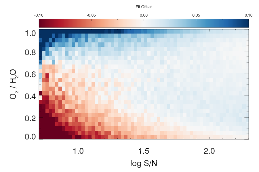
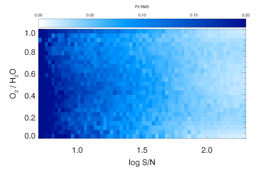
The best-fit and true values of and are compared as a function of S/N in Figure 4. These images are two-dimensional histograms, where the color bars display the mean offset between the best-fit and true values in a given bin. Systematic offsets are present in both and when , but are quite modest at the higher S/N values typical of our appulse observations (see Table 4). Figure 5 is similar to Figure 4, except its color bars display the RMS deviations between the best-fit and true values in a given bin after correcting for the systematic offsets in Figure 4. These deviations quantify the spread in true values that are associated with a particular best-fit value.
The “adopted” values of and are derived from our Monte Carlo simulations by identifying the 1,000 simulated spectra with S/N and best-fit values closest to those measured for a given observation, and fitting a Gaussian to the distribution of true values. We treat the mean of this Gaussian as the adopted value, and its standard deviation as the uncertainty. Since our fits constrain the allowable range of , we quote limits whenever the adopted value is from these boundaries.

The last two columns of Table 4 list the adopted values of and , respectively, for our stellar appulse observations. Figure 6 shows absorption profiles of and and their associated 95% () confidence bands using the adopted values for the appulse of HD 26912. These profiles are overlaid on the normalized stellar spectrum as in Figure 3, along with confidence bands for the sum of all other modeled species and the total absorption from all species. These profiles clearly show that the adopted values of and are consistent with the data. Absorption profiles derived from the adopted values for all targeted and serendipitous appulses are presented in Appendix B.
4 Discussion
4.1 Column Densities
The Monte Carlo simulations presented in Section 3.1 are one way to gain confidence in the validity of our absorption fits. Another is to compare our column densities with values measured by other instruments on Rosetta at similar times. Figure 7 shows the adopted values of for our stellar appulse observations as a function of , compared to the VIRTIS-H measurements of Bockelée-Morvan et al. (2016). Despite the large scatter in the column densities for a given value of , the adopted values for our appulse observations are reassuringly similar to the measured values from VIRTIS. One reason for the differences that do exist is the fact that the VIRTIS measurements were taken at systematically lower impact parameters than the appulses, as shown in the top panel of Figure 7.
While the values from Alice and VIRTIS are in good agreement, there may be discrepancies with the ROSINA measurements. Fougere et al. (2016) present a sophisticated Direct Simulation Monte Carlo (DSMC) model of the major species (, , CO, and ) in the coma of 67P/C-G, which derives molecular production rates from a non-uniform surface activity distribution. The DSMC model does a remarkable job of reproducing the in-situ ROSINA measurements of the number density of these species for all data taken before March 2016 (Fougere et al., 2016). However, when the model production rates are used to predict the values along the lines of sight probed by Bockelée-Morvan et al. (2016), it finds model column densities that are four times higher than those measured by VIRTIS (Fougere et al., 2016). The cause of this discrepancy is unclear, which illustrates the difficulty of directly comparing measurements from in-situ instruments such as ROSINA to those from remote-sensing instruments such as VIRTIS and Alice.
4.2
Figure 8shows the relative abundance of with respect to (top panel) and the column density of (bottom panel) as a function of . Figure 9 shows the same quantities as a function of impact parameter. The relative abundance tends to increase with increasing heliocentric distance and increasing impact parameter. These correlations ( and significance, respectively, according to Kendall’s tau test) cause the distributions of as a function of and to be flatter than the corresponding distributions of shown in Figure 7.
The relatively flat distribution of as a function of is particularly interesting, as it suggests a distributed source of . This would seem to argue against the variety of mechanisms that Mousis et al. (2016) suggest for trapping in the icy matrix of 67P/C-G. Formation of through the dismutation of during the evaporation of ice, as suggested by Dulieu et al. (2017), might be able to explain the shape of the distribution as a function of . Interestingly, ROSINA detects in the coma of 67P/C-G (see Figure 4 of Le Roy et al., 2015, and Figure 4 of Bieler et al., 2015), but with a relative abundance of % (Bieler et al., 2015), far less than the ratio of predicted by the dismutation reaction (Dulieu et al., 2017).
Feldman et al. (2016) used Alice to study gaseous outbursts in the coma of 67P/C-G. These outbursts exhibit no increase in long-wavelength solar reflected light that would indicate an increase in dust production, and are characterized by a sudden increase in the brightness ratio of O i in the sunward coma. Feldman et al. (2016) infer that these outbursts are driven by release, and estimate that % during the outbursts.
Coincidentally, our earliest archival appulse (HD 26912; see Figure 3 and Figure 6) occurred during the onset of one of the Feldman et al. (2016) outbursts (see their Section 2.5). We adopt % for this appulse (see Table 4), which is somewhat lower than the Feldman et al. (2016) estimate. This apparent discrepancy is likely a result of timing differences; i.e., the adopted value from the appulse measures the ambient in the coma just prior to outburst, whereas the Feldman et al. (2016) value measures the peak over the -minute duration of the outburst.
As mentioned in Section 3, the values in Table 4 are generally higher, and have considerably larger scatter, than the values found by ROSINA-DFMS. Bieler et al. (2015) found % in data taken between August 2014 and March 2015, and Fougere et al. (2016) found % throughout the time frame of our appulse observations. Notably, neither Bieler et al. (2015) nor Fougere et al. (2016) list a single observation where %, but we find a median value of 25%.
As discussed in Section 4.1, comparisons between the in-situ measurements of ROSINA and the line-of-sight measurements of Alice and VIRTIS are not straightforward, even with a sophisticated coma model (Fougere et al., 2016). Nonetheless, the large values of derived from the Alice data are surprising. While we have included several minor species in our absorption fits (see Section 3), there are many species detected in the coma of 67P/C-G by ROSINA for which we were unable to find absorption cross sections (Le Roy et al., 2015, e.g., HS, , ;). Some of these “missing” species could have cross sections large enough to cause measurable far-UV absorption, even for very small column densities, causing the current values to be over-estimated. Quantifying the magnitude of these systematic uncertainties is exceedingly difficult without additional laboratory data for far-UV molecular absorption cross sections.
Further, even if our fits currently include all of the relevant species, the absorption cross sections we use were all measured at K (see Table 3). Since the absorbing coma gas is expected to be at lower temperature, variations in the absorption cross sections with temperature could lead us to infer incorrect values of the column density with our current procedure. However, the scant existing data suggest that our procedure under-estimates the amount of low-temperature present by assuming room-temperature cross sections (Yoshino et al., 2005, see discussion in Section 3;), which would serve to increase the discrepancy between our results and those of ROSINA.
5 Conclusions
Using the Alice far-UV imaging spectrograph aboard Rosetta, we have independently verified the presence of in the coma of Comet 67P/C-G. was detected for the first time in the coma of a comet by Rosetta’s ROSINA mass spectrometer (Bieler et al., 2015; Fougere et al., 2016). In the present study, both and were detected in far-UV absorption against the continuum of stars located near the nucleus of 67P/C-G, at impact parameters of 4-20 km. These stellar appulses occurred at heliocentric distances of to 2.3 AU, where negative distances indicate pre-perihelion observations. The main results of our analysis are as follows:
- 1.
The column densities derived from the stellar spectra are in good agreement with VIRTIS-H measurements from the same time period taken at similar impact parameters (Bockelée-Morvan et al., 2016).
- 2.
The median value for the relative abundance of with respect to derived from the stellar spectra is %. This value is considerably higher than those reported by ROSINA; Bieler et al. (2015) and Fougere et al. (2016) found mean values of %.
We see no simple explanation for the difference in measured by Alice and ROSINA, unless it is related to the unmodeled species and K cross sections discussed at the end of Section 4.2. The Alice measurements are consistent with values published by other remote-sensing instruments on Rosetta; and while this does not guarantee that our values are correct it does suggest that our measurements are reasonably robust. The ROSINA measurements, on the other hand, are performed in situ at the spacecraft location, and the sophisticated coma model of Fougere et al. (2016) is designed to reproduce these measurements. This same model has difficulty reproducing the column densities of Bockelée-Morvan et al. (2016), which were measured very close to perihelion (Fougere et al., 2016). There is clearly much future work to be done to reconcile these differences.
Acknowledgements
Rosetta is an ESA mission with contributions from its member states and NASA. We thank the members of the Rosetta Science Ground System and Mission Operations Center teams, in particular Richard Moissl and Michael Küppers, for their expert and dedicated help in planning and executing the Alice observations. The Alice team acknowledges continuing support from NASA via Jet Propulsion Laboratory contract 1336850 to the Southwest Research Institute. This research has made use of the SIMBAD database, operated at CDS, Strasbourg, France.
References
- Ackerman et al. (1970) Ackerman M., Biaume F., Kockarts G., 1970, Planet. Space Sci., 18, 1639
- Acton (1996) Acton C. H., 1996, Planet. Space Sci., 44, 65
- Balsiger et al. (2007) Balsiger H. et al., 2007, Space Sci. Rev., 128, 745
- Barucci et al. (2016) Barucci, M. A. et al., 2016, A&A, 595, A102
- Bieler et al. (2015) Bieler A. et al., 2015, Nature, 526, 678
- Bockelée-Morvan et al. (2016) Bockelée-Morvan D. et al., 2016, MNRAS, 462, S170
- Brion & Tan (1979) Brion C. E., Tan K. H., 1979, J. Electron Spectrosc. Related Phenomena, 17, 101
- Cairns & Samson (1965) Cairns R. B., Samson J. A. R., 1965, J. Geophys. Res., 70, 99
- Chan et al. (1993) Chan W. F., Cooper G., Brion C. E., 1993, Chem. Phys., 178, 401
- Chung et al. (2001) Chung C.-Y., Chew E. P., Cheng B.-M., Bahou M., Lee Y.-P., 2001, Nuclear Instrum. Methods Phys. Res. A, 467-468, 1572
- Coradini et al. (2007) Coradini A. et al., 2007, Space Sci. Rev., 128, 529
- Ditchburn (1955) Ditchburn R. W., 1955, Proc. R. Soc. Lond., 229, 44
- Dulieu et al. (2017) Dulieu F., Minissale M., Bockelée-Morvan D., 2017, A&A, 597, A56
- Fahr & Nayak (1994) Fahr A., Nayak A. K., 1994, Chem. Phys., 189, 725
- Feldman et al. (2015) Feldman P. D. et al., 2015, A&A, 583, A8
- Feldman et al. (2016) Feldman P. D. et al., 2016, ApJ, 825, L8
- Fougere et al. (2016) Fougere N. et al., 2016, MNRAS, 462, S156
- Gentieu & Mentall (1970) Gentieu E. P., Mentall J. E., 1970, Science, 169, 681
- Gulkis et al. (2007) Gulkis S. et al., 2007, Space Sci. Rev., 128, 561
- Hitchcock et al. (1980) Hitchcock A. P., Brion C. E., van der Wiel M. J., 1980, Chem. Phys., 45, 461
- Huebner & Mukherjee (2015) Huebner W. F., Mukherjee J., 2015, Planet. Space Sci., 106, 11
- Koch & Skibowski (1971) Koch E. E., Skibowski M., 1971, Chem. Phys. Lett., 9, 429
- Le Roy et al. (2015) Le Roy, L. et al., 2015, A&A, 583, A1
- Lee et al. (2015) Lee, S. et al., 2015, A&A, 583, A5
- Lombos et al. (1967) Lombos B. A., Sauvageau P., Sandorfy C., 1967, J. Molecular Spectrosc., 24, 253
- Markwardt (2009) Markwardt C. B., 2009, in Bohlender D. A., Durand D., Dowler P., eds, ASP Conf. Ser. 411, Astronomical Data Analysis Software and Systems XVIII. Astron. Soc. Pac., San Francisco, p. 251
- Mentall et al. (1971) Mentall J. E., Gentieu E. P., Kraus M., Neumann D., 1971, J. Chem. Phys., 55, 5471
- Metzger & Cook (1964) Metzger P. H., Cook G. R., 1964, J. Chem. Phys., 41, 642
- Mota et al. (2005) Mota R. et al., 2005, Chem. Phys. Lett., 416, 152
- Mount & Moos (1978) Mount G. H., Moos H. W., 1978, ApJ, 224, L35
- Mousis et al. (2016) Mousis, O. et al., 2016, ApJ, 823, L41
- Nakayama & Watanabe (1964) Nakayama T., Watanabe K., 1964, J. Chem. Phys., 40, 588
- Okabe (1981) Okabe H., 1981, J. Chem. Phys., 75, 2772
- Okabe & Becker (1963) Okabe H., Becker D. A., 1963, J. Chem. Phys., 39, 2549
- Rubin et al. (2015) Rubin M., Altwegg K., van Dishoeck E. F., Schwehm G., 2015, ApJ, 815, L11
- Schoen (1962) Schoen R. I., 1962, J. Chem. Phys., 37, 2032
- Stark et al. (2007) Stark G., Yoshino K., Smith P. L., Ito K., 2007, J. Quant. Spectrosc. Radiative Transfer, 103, 67
- Stern et al. (2007) Stern S. A. et al., 2007, Space Sci. Rev., 128, 507
- Sun & Weissler (1955) Sun H., Weissler G. L., 1955, J. Chem. Phys., 23, 1160
- Taquet et al. (2016) Taquet V., Furuya K., Walsh C., van Dishoeck E. F., 2016, MNRAS, 462, S99
- Watanabe & Zelikoff (1953) Watanabe K., Zelikoff M., 1953, J. Opt. Soc. America, 43, 753
- Watanabe & Jursa (1964) Watanabe K., Jursa A. S., 1964, J. Chem. Phys., 41, 1650
- Wenger et al. (2000) Wenger M. et al., 2000, A&AS, 143, 9
- Yoshino et al. (1996) Yoshino K., Esmond J. R., Sun W. H., Parkinson W. H., Ito K., Matsui T., 1996, J. Quant. Spectrosc. Radiative Transfer, 55, 53
- Yoshino et al. (2005) Yoshino K., Parkinson W. H., Ito K., Matsui T., 2005, J. Molecular Spectrosc., 229, 238
- Zelikoff & Watanabe (1953) Zelikoff M., Watanabe K., 1953, J. Opt. Soc. America, 43, 756
Appendix A Best-Fit Absorption Profiles
Figures 10-38 present best-fit absorption profiles for all targeted and archival stellar appulses, arranged chronologically. The top panel of each figure displays the normalized stellar flux (black) and uncertainty (gray), with best-fit ensemble absorption (solid brown line) overlaid. Absorption from individual species is shown with solid (, , CO, , ) or dashed (, , , , ) lines. The bottom panel of each figure displays the residual of the ensemble fit.
Appendix B Adopted Absorption Profiles
Figures 39-67 present the adopted column densities for all targeted and archival stellar appulses, with 95% () confidence bands. The top panel of each figure displays the normalized stellar flux and associated 95% confidence band (gray), with ensemble fit (brown) and individual-species absorption overlaid using the adopted column densities of and from Table 4. The bottom panel of each figure displays the residual of the ensemble fit.


