Joint Fractional Time Allocation and Beamforming for Downlink Multiuser MISO Systems Thanks: This work was supported in part by the National Research Foundation of Korea (NRF) grant funded by the Korean government (MSIT) (No. NRF-2017R1A5A1015596), in part by Basic Science Research Program through the NRF funded by the Ministry of Education (No. 2017R1D1A1B03030436), in part by the U.K. Royal Academy of Engineering Research Fellowship under Grant RF1415$/\penalty$14$/\penalty$22 and by the U.K. Engineering and Physical Sciences Research Council (EPSRC) under Grant EP/P019374/1, and in part by the KAUST Grant No. OSR-2016-CRG5-2958-0 and U.S. National Science Foundation Grant ECCS-1647198. (Corresponding author: Oh-Soon Shin.)

In multi-user communication, the signal received by any user (UE) is a superposition of the desired information and the information intended for other UEs. Transmit beamforming at a base station (BS) plays a pivotal role in focusing the energy of the desired signal and suppressing the multi-user interference to achieve better throughput at UEs [1, 2]. For effective beamforming, the number of UEs usually does not exceed the number of transmit antennas. Using more transmit antennas and thus increasing the dimensionality of beamforming vectors can improve the UEs’ throughput with reduced transmit power. However, allocating more transmit power under fixed number of transmit antennas still does not necessarily improve the UEs’ throughput.

Non-orthogonal multiple access (NOMA) [3, 4] has been introduced to improve the UEs’ throughput by allowing UEs with better channel conditions to access and decode the signals, which are intended for the UEs with poorer channel conditions. In other words, the UEs with poorer channel conditions can achieve higher throughput by compromising their information privacy in NOMA [5]. This privacy compromise for the UEs with poor channel conditions is unavoidable in NOMA. Moreover, by restricting all beamforming vectors in the same space, beamforming in NOMA still needs that the dimension of this space, which is equal to the number of transmit antennas, should not be less than the number of UEs to allow the suppression of multiuser interference [6].

It is noteworthy that the UEs with good channel conditions may need only a fraction of the time unit to achieve their needed throughput. Therefore, by serving them only per fractional time, the BS still has the remaining time room to serve the UEs with poor channel conditions. In this way, the information privacy for each UE is preserved because all UEs are allowed to decode their own information only. More importantly, the number of UEs supported at the same fractional time is effectively reduced. Thus, the BS will not need more transmit antennas to suppress the multi-user interference. In this letter, the fractional time allocation to UEs with similar channel conditions and beamforming are enhanced for improving the system’s throughput and meeting the UEs’ quality-of-service (QoS) in terms of the throughput requirement. This problem is mathematically modelled by a highly nonconvex optimization problem, for which a path-following computational procedure of low complexity is then developed for its computation. Finally, the numerical examples are provided to demonstrate the advantage of the proposed optimization scheme.

Notation. We use bold upper-case letters for matrices, bold lower-case letters for column vectors, lower-case letters for scalars. $\Re\{x\}$ denotes the real part of a complex number $x$. The notation $(\cdot)^{H}$ stands for the Hermitian transpose. $\mathbf{x}\sim\mathcal{CN}(\boldsymbol{\eta},\boldsymbol{Z})$ means that $\mathbf{x}$ is a random vector following a complex circular Gaussian distribution with mean $\boldsymbol{\eta}$ and covariance matrix $\boldsymbol{Z}$.

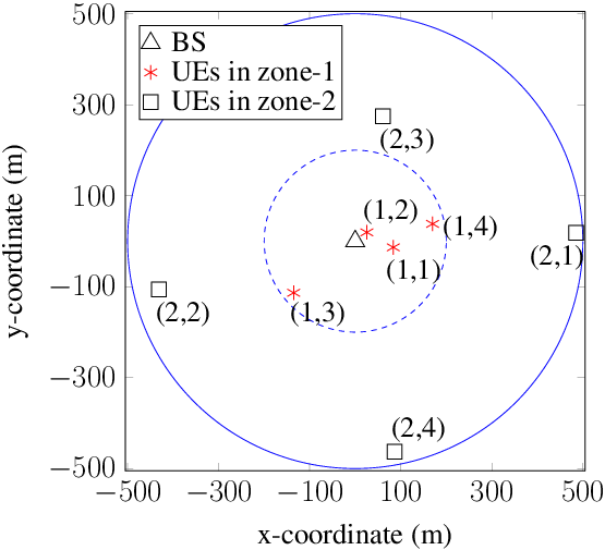
Consider a multiuser downlink system over a given frequency band with a BS equipped with $N_{t}>1$ antennas in serving $2K$ single-antenna UEs as illustrated by Fig. 1. There are $K$ UEs $(1,k)$, $k=1,\dots K$, which are located in a zone nearer to the BS, called by zone-1, and $K$ UEs $(2,k)$, $k=1,\dots,K$, which are located in a zone farer from the BS, called by zone-2. Denote by $\mathcal{K}\triangleq\{1,2,\dots,K\}$ and $\mathcal{M}=\{1,2\}\times\mathcal{K}$. Within one time unit, BS uses the fraction time (FT) $\tau_{1}:=\tau\;(0<\tau<1)$ to serve UEs $(1,k)$ and uses the remaining FT $\tau_{2}:=(1-\tau)$ to serve UEs $(2,k)$.

The BS deploys a transmit beamformer $\mathbf{w}_{i,k}\in\mathbb{C}^{N_{t}\times 1}$ to deliver the information signal $x_{i,k}$ with $\mathbb{E}\{|x_{i,k}|^{2}\}=1$ to UE $(i,k)$. Let $\mathbf{h}_{i,k}\in\mathbb{C}^{N_{t}\times 1}$ be the channel vector from the BS to UE $(i,k)$, which is assumed to follow frequency flat fading with the effects of both large-scale pathloss and small-scale fading counted. The complex baseband signal received by UE $(i,k)$ can be expressed as

where the first term is the desired signal, the second term is the multi-user interference, and the third term $n_{i,k}\sim\mathcal{CN}(0,\sigma^{2}_{i,k})$ is additive noise. For $\mathbf{w}_{i}\triangleq(\mathbf{w}_{i,k})_{k\in{\cal K}}$, the throughput at UE $(i,k)$ is

which by [7] can be equivalently reformulated by

under the additional condition

The main advantage of this FT-based beamforming scheme is that there is no inter-zone interference in (1) that is in contrast with the conventional scheme to concurrently serve all UEs, under which the throughput at UE $(i,k)$ is

with the full inter-zone interference. Here and in the sequence $\mathbf{w}\triangleq(\mathbf{w}_{1},\mathbf{w}_{2})$ and $\boldsymbol{\tau}\triangleq(\tau_{1},\tau_{2})$.

We are interested in the following problem of jointly designing FT $(\tau_{1},\tau_{2})$ and the beamformers $(\mathbf{w}_{1},\mathbf{w}_{2})$ to maximize the system sum throughput (ST):

Here ${\mathsf{\bar{R}}}_{i,k}$ sets a minimum throughput requirement for UE $(i,k)$ and $P_{bs}^{\max}$ is a given power budget. Since ${\cal R}_{i,k}(\mathbf{w}_{i},\tau_{i})$ is a nonconcave function, the optimization problem (4) is regarded as a highly nonconvex optimization problem, for which finding a feasible point is already computationally difficult. The next section is devoted to a computational path-following procedure for its solution.

The most important step is to provide an effective lower bounding approximation for the function ${\cal R}_{i,k}(\mathbf{w}_{i},\tau_{i})$ defined by (1) to facilitate a path-following computational procedure of the problem (4). We use the variable changes $\boldsymbol{\alpha}\triangleq(\alpha_{1},\alpha_{2})=(1/\tau_{1},1/\tau_{2})$, which satisfy the following convex constraint:

The problem (4) can be equivalently expressed as

At a feasible point $(\mathbf{w}^{(\kappa)},\boldsymbol{\alpha}^{(\kappa)})$, define $x_{i,k}^{(\kappa)}\triangleq\Re\{\mathbf{h}_{i,k}^{H}\mathbf{w}_{i,k}^{(\kappa)}\}>0$, $y_{i,k}^{(\kappa)}\triangleq\sum_{j\in\mathcal{K}\setminus\{k\}}|\mathbf{h}_{i,k}^{H}\mathbf{w}_{i,j}^{(\kappa)}|^{2}+\sigma^{2}_{i,k}$, $d_{i,k}^{(\kappa)}\triangleq(x_{i,k}^{(\kappa)})^{2}/y_{i,k}^{(\kappa)}>0$, $a^{(\kappa)}_{i,k}\triangleq 2{\cal R}_{i,k}(\mathbf{w}_{i}^{(\kappa)},1/\alpha_{i}^{(\kappa)})+d_{i,k}^{(\kappa)}/\alpha_{i}^{(\kappa)}(d_{i,k}^{(\kappa)}+1)>0$, $b^{(\kappa)}_{i,k}\triangleq(d_{i,k}^{(\kappa)})^{2}/\alpha_{i}^{(\kappa)}(d_{i,k}^{(\kappa)}+1)>0$, and $c_{i,k}^{(\kappa)}\triangleq{\cal R}_{i,k}(\mathbf{w}_{i}^{(\kappa)},1/(\alpha_{i}^{(\kappa)})^{2})>0$. It follows from the inequality (13) in the appendix that

over the trust region

for the concave function

Next, due to the convexity of function $\|\mathbf{w}_{1}\|^{2}/\alpha_{2}$, it is true that $\|\mathbf{w}_{1}\|^{2}/\alpha_{2}\geq 2\Re\{(\mathbf{w}_{1}^{(\kappa)})^{H}\mathbf{w}_{1}\}/\alpha_{2}^{(\kappa)}-(\|\mathbf{w}_{1}^{(\kappa)}\|^{2}/(\alpha_{2}^{(\kappa)})^{2})\alpha_{2}$. An inner convex approximation of nonconvex constraint (6c) is then given by

Initialized by a feasible point $(\mathbf{w}^{(0)},\boldsymbol{\alpha}^{(0)})$ for (6), the following convex quadratic program (QP) is solved at the $\kappa$-th iteration to generate the next feasible point $(\mathbf{w}^{(\kappa+1)},\boldsymbol{\alpha}^{(\kappa+1)})$:

As problem (9) involves $m=2(3K+1)$ quadratic and linear constraints, and $n=2(KN_{t}+1)$ real decision variables, its computational complexity is $\mathcal{O}(n^{2}m^{2.5}+m^{3.5})$.

Note that $\Phi(\mathbf{w},\boldsymbol{\alpha})\geq\Phi^{(\kappa)}(\mathbf{w},\boldsymbol{\alpha})$ $\forall(\mathbf{w},\boldsymbol{\alpha})$, and $\Phi(\mathbf{w}^{(\kappa)},\boldsymbol{\alpha}^{(\kappa)})=\Phi^{(\kappa)}(\mathbf{w}^{(\kappa)},\boldsymbol{\alpha}^{(\kappa)})$. Moreover, $\Phi^{(\kappa)}(\mathbf{w}^{(\kappa+1)},\boldsymbol{\alpha}^{(\kappa+1)})>\Phi^{(\kappa)}(\mathbf{w}^{(\kappa)},\boldsymbol{\alpha}^{(\kappa)})$ whenever $(\mathbf{w}^{(\kappa+1)},\boldsymbol{\alpha}^{(\kappa+1)})\neq(\mathbf{w}^{(\kappa)},\boldsymbol{\alpha}^{(\kappa)})$ because the former and the latter, respectively, are the optimal solution and feasible point for (9). Therefore, $\Phi(\mathbf{w}^{(\kappa+1)},\boldsymbol{\alpha}^{(\kappa+1)})\geq\Phi^{(\kappa)}(\mathbf{w}^{(\kappa+1)},\boldsymbol{\alpha}^{(\kappa+1)})>\Phi^{(\kappa)}(\mathbf{w}^{(\kappa)},\boldsymbol{\alpha}^{(\kappa)})=\Phi(\mathbf{w}^{(\kappa)},\boldsymbol{\alpha}^{(\kappa)})$, showing that $(\mathbf{w}^{(\kappa+1)},\boldsymbol{\alpha}^{(\kappa+1)})$ is a better feasible point than $(\mathbf{w}^{(\kappa)},\boldsymbol{\alpha}^{(\kappa)})$ for (6). The sequence $\{(\mathbf{w}^{(\kappa)},\boldsymbol{\alpha}^{(\kappa)})\}$ of improved feasible points for (6) thus converges at least to a locally optimal solution satisfying the Karush-Kuh-Tucker conditions [8]. We summarize the proposed QP-based path-following procedure in Algorithm 1.

Generation of an initial point.: Initialized from a feasible point $(\mathbf{w}^{(0)},\boldsymbol{\alpha}^{(0)})$ for constraints (5) and (8), we iterate the convex program

till reaching $\min_{(i,k)\in{\cal M}}{\cal R}_{i,k}^{(\kappa)}(\mathbf{w}_{i}^{(\kappa+1)},\alpha_{i}^{(\kappa+1)})/\bar{\mathsf{R}}_{i,k}\geq 1$ to make $(\mathbf{w}^{(\kappa+1)},\boldsymbol{\alpha}^{(\kappa+1)})$ feasible for (6) and thus usable as an initial feasible point for implementing Algorithm 1.

Monte Carlo simulations have been implemented to evaluate the performance of the proposed algorithm for $K=4$ ($8$ UEs) and $N_{t}=5$ per the scenario in Fig. 1. The channel vector $\mathbf{h}_{i,k}$ between the BS and UE $(i,k)$ at a distance $d_{i,k}$ (in kilometres) is generated as $\mathbf{h}_{i,k}=\sqrt{10^{-\sigma_{\mathsf{PL}}/10}}\tilde{\mathbf{h}}_{i,k}$, where $\sigma_{\mathsf{PL}}$ is the path loss (PL) in dB and $\tilde{\mathbf{h}}_{i,k}\sim\mathcal{CN}(0,\mathbf{I}_{N_{t}})$ represents small-scale effects. The other parameters are given by Table I. Without loss of generality, $\bar{\mathsf{R}}_{i,k}\equiv\bar{\mathsf{R}}$ is set. The numerical results are obtained using the parser YALMIP [9].

We compare the performance of the proposed FT-based beamforming scheme with five other beamforming schemes: $(i)$ “Conventional DL,” under which the problem of ST maximization is formulated similarly as: $\max_{\mathbf{w}}\sum_{(i,k)\in{\cal M}}{\cal R}_{i,k}^{{}^{\prime}}(\mathbf{w})\ {\mathrm{s.t.}}\ {\cal R}_{i,k}^{{}^{\prime}}(\mathbf{w})\geq{\mathsf{\bar{R}}}_{i,k},(i,k)\in{\cal M},\|\mathbf{w}_{1}\|^{2}+\|\mathbf{w}_{2}\|^{2}\leq P_{bs}^{\max}$ under the definition (3); $(ii)$ “NOMA”: each UE in zone-1 is paired with an UE in zone-2 according to the clustering algorithm in [10] to create a virtual cluster. In each cluster, both UEs decode the signal intended for the UE in zone-2 and then the UE in zone-1 processes successive interference cancellation (SIC) to cancel the interference of the UE in zone-2 in decoding its own signal; $(iii)$ “FT + NOMA in both zones”: under FT, NOMA is zone-wide adopted; $(iv)$ “FT + NOMA in zone-1”: under FT, NOMA is adopted only in zone-1; and $(v)$ “FT + NOMA in zone-2”: under FT, NOMA is adopted only in zone-2. The reader is referred to [6, Sec. V] for beamforming under NOMA, which is used in these five schemes. The computational complexity of each iteration in NOMA is similar to that of (9). Note that the performance of NOMA-based beamforming can be improved by involving more UEs in virtual clusters [6, Sec VI] but the UEs’ privacy is more compromised.

On average, Algorithm 1 requires about $10$ iterations for convergence.

Fig. 2 plots the average achievable ST versus the transmit power $P_{bs}^{\max}$ for $N_{t}=5$. For $\bar{\mathsf{R}}=0$ bps/Hz shown in Fig. 2(a), one can see that the ST of the proposed FT-based beamforming is higher than that achieved by the other schemes in the high transmit power region. On the other hand, the conventional DL outperforms NOMA and FT+NOMA schemes for high transmit power by making the ST concentrated at those UEs with good channel conditions. Apparently, NOMA does not look efficient when there is no UEs’ QoS requirement. In Fig. 2(b) with $\bar{\mathsf{R}}=1$ bps/Hz, the conventional DL performs worse than NOMA at high $P_{bs}^{\max}$. The low STs of FT+NOMA-based schemes are probably attributed to the fact that NOMA is more efficient by exploiting their channel differentiation. Increasing $P_{bs}^{\max}$ leads to a remarkable gain in ST by the proposed FT compared with the other schemes. In addition, the proposed FT is feasible in all range of $P_{bs}^{\max}$ while the other schemes cannot offer such high QoS to UEs at low $P_{bs}^{\max}$.

The plot of the ST versus QoS requirement threshold $\bar{\mathsf{R}}\in[0.2,\;1.2]$ bps/Hz is illustrated in Fig. 3. We can observe that the proposed FT-based beamforming performs quite well and only slightly degrades when $\bar{\mathsf{R}}$ increases. The performance gap between the proposed FT-based beamforming and other schemes substantially increases by increasing $\bar{\mathsf{R}}$. It is expected because the proposed FT-based beamforming can tune the power allocation in meeting zone-2 UEs’ QoS requirements without causing interference to the zone-1’s UEs.

Next, we look for the max-min UE throughput optimization problem

which can be addressed similarly by solving the convex program (10) (with $\bar{\mathsf{R}}_{i,k}\equiv 1$) at each iteration.

Fig. 4 plots the average UEs’ worst throughput as a function of $P_{bs}^{\max}$. It shows that the worst throughput achieved by the conventional DL and FT + NOMA-based schemes is saturated once $P_{bs}^{\max}$ is beyond a threshold. It also reveals that the proposed FT-based beamforming and FT + NOMA in zone-1 achieve worst throughput that is higher than that achieved by others schemes.

The paper has proposed a fractional time-based beamforming scheme at a base station to serve two groups of users, which is able to improve the network throughput while preserving the information privacy for the users. Accordingly, a path-following computational procedure for the joint design of fractional times and beamforming vectors to maximize the network throughput has been developed. Extensive simulations have been provided to demonstrate the superior performance of the proposed scheme over the exiting schemes.

For all $x>0$, $\bar{x}>0$, $y>0$, $\bar{y}>0$, $t>0$, and $\bar{t}>0$, it is true that

over the trust region

where $a=2[\ln(1+d)]/\bar{t}+d/\bar{t}(d+1)>0,b=d^{2}/\bar{t}(d+1)>0,\\ c=[\ln(1+d)]/\bar{t}^{2}>0,d=\bar{x}^{2}/\bar{y}.$ Inequality (12) follows from [11] while inequality (13) is obtained by using $x^{2}\geq\bar{x}(2x-\bar{x})>0$ over the trust region (14).

References

- [1] X. Shang, B. Chen, and H. V. Poor, “Multiuser MISO interference channels with single-user detection: Optimality of beamforming and the achievable rate region,” IEEE Trans. Inf. Theory, vol. 57, no. 7, pp. 4255–4273, July 2011.
- [2] G. Caire and S. Shamai, “On the achievable throughput of a multiantenna Gaussian broadcast channel,” IEEE Trans. Inf. Theory., vol. 49, no. 7, pp. 1691 – 1706, July 2003.
- [3] Z. Ding, R. Schober, and H. V. Poor, “A general MIMO framework for NOMA downlink and uplink transmission based on signal alignment,” IEEE Trans. Wireless Commun., vol. 15, no. 6, pp. 4483–4454, June 2016.
- [4] Z. Ding, Y. Liu, J. Choi, Q. Sun, M. Elkashlan, C. L. I, and H. V. Poor, “Application of non-orthogonal multiple access in LTE and 5G networks,” IEEE Commun. Mag., vol. 55, no. 2, pp. 185–191, Feb. 2017.
- [5] Z. Ding, F. Adachi, and H. V. Poor, “The application of MIMO to non-orthogonal multiple access,” IEEE Trans. Wireless Commun., vol. 15, no. 1, pp. 537–552, Jan. 2016.
- [6] V.-D. Nguyen, H. D. Tuan, T. Q. Duong, H. V. Poor, and O.-S. Shin, “Precoder design for signal superposition in MIMO-NOMA multicell networks,” IEEE J. Select. Areas Commun., 2017, to appear, available at http://ieeexplore.ieee.org/stamp/stamp.jsp?tp=arnumber=7974739.
- [7] A. Wiesel, Y. Eldar, and S. Shamai, “Linear precoding via conic optimization for fixed MIMO receivers,” IEEE Trans. Signal Process., vol. 54, no. 1, pp. 161 – 176, Jan. 2006.
- [8] B. R. Marks and G. P. Wright, “A general inner approximation algorithm for nonconvex mathematical programms,” Operations Research, vol. 26, no. 4, pp. 681–683, July 1978.
- [9] J. Lfberg, “YALMIP: A toolbox for modeling and optimization in MATLAB,” in Proc. 2004 IEEE Inter. Symposium on Computer Aided Control Systems Design, Sept. 2004, pp. 284–289.
- [10] B. Kimy, S. Lim, H. Kim, S. Suh, J. Kwun, S. Choi, C. Lee, S. Lee, and D. Hong, “Non-orthogonal multiple access in a downlink multiuser beamforming system,” in Proc. IEEE Military Commun. Conf. (MILCOM), Nov. 2013, pp. 1278–1283.
- [11] V.-D. Nguyen, T. Q. Duong, H. D. Tuan, O.-S. Shin, and H. V. Poor, “Spectral and energy efficiencies in full-duplex wireless information and power transfer,” IEEE Trans. Commun., vol. 65, no. 5, pp. 2220–2233, May 2017.