Hybrid Beamforming with Reduced Number of Phase Shifters for Massive MIMO Systems

Massive multiple-input multiple-output (MIMO) technology with digital beamforming can increase the spectral efficiency in wireless communication systems. However, a dedicated RF chain per antenna increases the cost of this technology. In order to reduce the number of RF chains, hard and soft antenna selection techniques have been proposed [1]. In the hard selection, the RF chains are connected to the antennas by a network of switches. The drawback of this approach is that large beamforming gains cannot be achieved as only a small fraction of the antennas are used [1, 2]. In the soft antenna selection, also known as hybrid beamforming, the RF chains and the antennas are connected through a network of phase shifters [3, 4, 1, 5]. Such architectures have lower cost and power consumption compared to digital beamformers and they achieve a higher spectral efficiency compared to hard selection. There are two types of phase shifter networks known as fully-connected and subconnected [5]. In the fully-connected structure, each RF chain is connected to all the antennas as in [3, 1, 4]. It can exploit the full array gain, however, its power consumption can be very high due to the massive number of the phase shifters it requires [3, 5]. In the subconnected configuration, each RF chain is connected to a subset of antennas which results in a simpler circuit but with lower spectral efficiency compared to that of the fully-connected configuration [5]. In general, the design of the optimal soft antenna selection schemes is a challenging task due to the nonconvex constant modulus constraint imposed by the phase shifters [5, 3, 1, 4]. In this context, [3, 6, 5] used switches that are cheaper and power efficient alternatives to phase shifters. Similar to the phase shifter networks, switch networks have fully-connected and subconnected structures. However, due to the requirement of large number of switches, a fully-connected configuration with switches has high hardware complexity and experiences insertion losses and cross talk distortion [7]. Hence, subconnected switch network,for example binary switches, is also preferred in practice despite the less degrees of freedom in antenna selection [7]. It is noted that the work in [4, 1, 5, 7, 6, 2], and references therein, only focus on antenna selection with either phase shifters or switches, and do not consider the combination of the two methods.

Recently, the authors in [8] used for the first time a combination of switches and non-tunable phase shifters to show that the spectral efficiency of hybrid beamforming with fully-connected phase shifter network can be achieved using such combination. While the approach in [8] requires a relatively low computational complexity and low power consumption, it demands a massive number of RF routes which could result in a complex hardware and high levels of crosstalk. Within the same context of designing the joint switches and phase-shifter based hybrid beamforming, [3] considers a fully-connected phase shifter network where each phase shifter was equipped with a switch. It was shown that it is possible to reduce the power consumption of the RF beamformer by turning off almost 50% of the phase shifters while achieving the same spectral efficiency. With the motivation to reduce the power consumption of massive MIMO systems while achieving high spectral efficiency, there is still a need for investigating new techniques to jointly design the beamforming weights at the baseband as well as the phase shifter and switch networks.

In this paper, two such novel combinations of phase shifters and switches are proposed and their performances in terms of the achievable sum-rate are evaluated. To this end, first we derive the closed-form expression of the beamformer and its achievable sum-rate over uncorrelated independent and identically distributed (i.i.d.) channel when the RF beamformer has subconnected structure. This approach offers lower computational complexity and similar performance compared to the successive interference cancellation based method in [5] when a small number of RF chains are connected to a large number of antennas. Second, based on the presented approach for the subconnected phase shifter network and using phase shifter selection technique, in [3], for fully-connected phase shifter network, it is shown that a combination of subconnected phase shifter and fully-connected switch networks can reduce the number of the phase shifters by 50% without any performance loss over uncorrelated i.i.d. Rayleigh fading channels. The simulation results for sparse scattering and correlated Rayleigh fading channels indicate that the achievable sum-rates almost remain at the same level when the number of the phase shifters are reduced to half. However, as the proposed structure requires a fully-connected switch network, which may not be suitable for practical applications, it is desirable to substitute the complex switch network with simpler structures, for example binary switches. Hence, we present another novel beamforming method that provides a slightly lower performance but with a much simpler hardware structure. In this approach, the fully-connected switches are replaced with simple subconnected switches, e.g. binary switches. Finally, the simulation results indicate that the asymptotic closed-form expressions of the spectral efficiency provide a good approximation of the performance for moderate number of antennas and phase shifters.

This paper is organized as following, the system model and hybrid beamforming with subconnected phase shifter network are described in sections II and III. In section IV, the proposed method for hybrid beamforming with subconnected phase shifters and fully-connected switches are presented. The analysis for the subconnected phase shifters that are connected to subconnected switch network are discussed in V. Finally, the simulation results and conclusion are presented in sections VI and VII.

Notations: Bold capital and small letters A and a represent a matrix and a vector, respectively. $A_{mn}$ denotes the $(m,n)$-th element of A, $\textbf{a}_{m}$ is the $m$-th column of A and $\textbf{A}_{1:m}$ is a matrix containing the first $m$ columns of A. det$(\textbf{A})$, $\textbf{A}^{\text{H}}$ and trace(A) denote determinant, Hermitian and trace of A, respectively. Moreover, $|A|$ and $\angle A$ denote the magnitude and angle of complex number $A$. $\textbf{I}_{m}$ is an $m\times m$ identity matrix. Finally, $f_{A}(a)$, $F_{A}(a)$ and E$[A]$ denote the probability density function (pdf), cumulative distribution function (cdf) and expected value of $A$, respectively.

In this work, a narrowband single-cell multiuser scenario in downlink where the base station with $N$ omni-directional antennas serves $K$ single-antenna users is considered. The wireless channel matrix $\textbf{H}\in\mathbb{C}^{K\times N}$ follows an uncorrelated Rayleigh fading model with i.i.d. elements as $H_{kn}\sim\mathcal{CN}(0,1),\>\forall k\in\{1,\>...,\>K\}$ and $\forall n\in\{1,\>...,\>N\}$. In this case, the relationship between the channel input vector $\textbf{x}\in\mathbb{C}^{N\times 1}$ and output vector $\textbf{y}\in\mathbb{C}^{K\times 1}$ is expressed as $\textbf{y}=\textbf{Hx}+\textbf{z}$ where $\textbf{z}\in\mathbb{C}^{K\times 1}$ is i.i.d. additive white Gaussian noise vector with $z_{k}\sim\mathcal{CN}(0,\sigma_{\text{z}}^{2})$ and noise variance of $\sigma_{\text{z}}^{2}$. It is assumed that the transmitter has perfect channel state information. A vector of $K$ symbols $\textbf{u}\in\mathbb{C}^{K\times 1}$ with E$[\textbf{uu}^{\text{H}}]=\textbf{I}_{K}$ are precoded using the precoding matrix F. Then, the signal at the transmitter antennas is $\textbf{x}=\sqrt{\frac{P}{\Gamma}}\textbf{Fu}$ where $P$ is the total transmit power per stream and $\Gamma=\text{E}\big[\text{trace}(\textbf{F}\textbf{F}^{\text{H}})\big]/K$ is a power normalization factor. Assuming that equal power is allocated to the users, the ergodic sum-capacity of downlink channel is [9]

In massive MIMO systems, it has been shown that linear precoders such as zero-forcing (ZF) can achieve a close to optimal performance [10]. Applying ZF precoding matrix $\textbf{H}^{\text{H}}(\textbf{HH}^{\text{H}})^{-1}$, the sum-rate becomes [3]

where $\Gamma_{\text{ZF}}=\text{E}\big[\text{trace}\big((\textbf{HH}^{\text{H}})^{-1}\big)\big]/K$ is the power normalization factor for ZF precoder. When H follows i.i.d. Rayleigh fading model, then $\Gamma_{\text{ZF}}=1/(N-K)$ as for central complex Wishart matrices it was shown that $\text{E}[\text{trace}\big((\textbf{HH}^{\text{H}})^{-1}\big)=K/(N-K)$ [11]. To maximize multiplexing gain in the high signal-to-noise ratio (SNR) regime, it is assumed that $M=K$ where $M$ is the number of the RF chains.

Figure 1a presents the diagram of a fully-connected antenna selection structure where each RF chain is connected to all antennas through a network of switches or phase shifters. Depending on the performance metric, e.g. maximizing the spectral efficiency, the hard antenna selection chooses the best $M$ out of $N$ antennas using its switching network. In this paper, a matrix that includes the state of the switches, i.e. on or off which are represented by zero and one, is referred as the select matrix. The disadvantage of hard antenna selection is that large array gains cannot be achieved when $M\ll N$. In general, soft antenna selection techniques provide a better performance compared to hard selection [3, 4, 1]. However, the fully-connected structure in Fig. 1a requires $MN$ switches or phase shifters which becomes very large in massive MIMO scenarios [5]. This introduces high insertion losses and hardware complexity. Hence, the subconnected configuration, as shown in Fig. 1b, is preferred in practice. The precoder matrix $\textbf{F}=\textbf{F}_{\text{sub}}\textbf{F}_{\text{B}}$ for the structure of Fig. 1b consists of a block diagonal RF beamforming matrix $\textbf{F}_{\text{sub}}\in\mathbb{C}^{N\times M}$ and a baseband precoder $\textbf{F}_{\text{B}}\in\mathbb{C}^{M\times K}$. The RF beamformer has to be designed such that the spectral efficiency $R_{\text{sub}}$ is maximized subject to $F_{\text{sub},nm}=\text{e}^{j\theta_{nm}},\>\forall\theta_{nm}\in[0,2\pi)$ and $\forall n\in\mathcal{I}_{m}$ where $\mathcal{I}_{m}=\{\frac{N}{M}(m-1)+1,...,\frac{N}{M}m\}$, otherwise $|F_{\text{sub},nm}|=0$. In this case, $\Gamma_{\text{sub}}=\big[\text{trace}(\textbf{F}_{\text{sub}}\textbf{F}_{\text{sub}}^{\text{H}})\big]/M=N/M$. In general, soft selection (hybird beamforming) is a challenging task as the maximization of the spectral efficiency is a nonconvex problem due to the constant modulus constraint imposed by the phase shifters [5, 3, 4, 1].

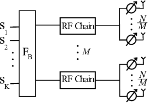
In this paper, firstly the closed-form expression for an asymptotically optimal beamformer will be presented. In order to reduce the power consumption of the structure in Fig. 1b, it will be shown that the configuration of Fig. 1c can replace 50% of the phase shifters with switches and without a performance loss. Finally, in Fig. 1d, we propose a simpler structure that the complicated fully-connected switch network is replaced with low-cost 1-out-of-$S$ switches where $S$ is the ratio of the number output-to-input ports.

The singular value decomposition (SVD) of the channel matrix is denoted as $\textbf{H}=\textbf{U}\boldsymbol{\Sigma}\textbf{V}^{\text{H}}$, where $\textbf{V}\in\mathbb{C}^{N\times N}$ and $\textbf{U}\in\mathbb{C}^{K\times K}$ contain the right and left singular vectors. The diagonal matrix $\boldsymbol{\Sigma}\in\mathbb{R}^{K\times N}$ includes the singular values of H. It is noted that $\textbf{H}=\textbf{U}\boldsymbol{\Sigma}_{1:M}\textbf{V}_{1:M}^{\text{H}}$ as H has only $M$ nonzero singular values. The statistical properties of the elements of V when $N\to\infty$ was analyzed in [3] and it was shown that

1. 1.

   $\sqrt{N}V_{nn^{\prime}}\sim\mathcal{CN}(0,1),\>\forall n,n^{\prime}\in\{1,\>...,\>N\}$ are i.i.d.,

2. 2.

   $|\sqrt{N}V_{nn^{\prime}}|$ is a Rayleigh variable with parameter $\frac{1}{\sqrt{2}}$,

3. 3.

   $\sqrt{N}\text{E}[|V_{nn^{\prime}}|]=\sqrt{\pi}/2$.

When the impact of the beamforming matrix of the subconnected phase shifter network is considered, the achievable sum-rate in (1) is expressed as

where (a) results from $\log_{2}$det$(\textbf{I}+\textbf{AB})=\log_{2}$ det$(\textbf{I}+\textbf{BA})$, $\Gamma_{\text{sub}}=N/M$, matrix Q is defined as $\textbf{Q}=\frac{M\textbf{V}_{1:M}^{\text{H}}\textbf{F}_{\text{sub}}\textbf{F}_{\text{sub}}^{\text{H}}\textbf{V}_{1:M}}{N}$, and the inequality $(b)$ comes from linear algebra as for any positive semidefinite matrix $\textbf{A}\in\mathbb{C}^{M\times M}$, $\text{det}(\textbf{A})\leq\prod_{m}A_{mm}$. If Q is a diagonal matrix, then $(b)$ in (3) turns into equality. Hence, $\textbf{F}_{\text{sub}}$ that upper bounds $R_{\text{sub}}$ should i) diagonalize $\textbf{Q}=\textbf{GG}^{\text{H}}$ where $\textbf{G}=\sqrt{M/N}\textbf{V}_{1:M}^{\text{H}}\textbf{F}_{\text{sub}}$. This requires $M/N|\textbf{v}_{m^{\prime}}^{\text{H}}\textbf{f}_{\text{sub},m}|^{2}=0$ when $m\neq m^{\prime}$ and $\forall m,m^{\prime}\in\{1,...,M\}$, ii) maximize the diagonal elements of $\textbf{GG}^{\text{H}}$. In Appendix A, it is shown that these conditions are held and (3) is maximized when

Moreover, according to Appendix A, using (4) results in

due to the law of large numbers. Similarly, $\lim_{N\to\infty}|\sqrt{N}\textbf{v}_{n}^{\text{H}}\textbf{f}_{\text{sub},m}|=0,\>\forall m\neq n$ as $\text{E}[\sqrt{N}V_{mn}]=0$.

Remark 1: The proposed RF beamformer in (4) for Fig. 1b, is derived under the assumption that $M$ is fixed and $L\to\infty$. Hence, it provides a suboptimal solution for relatively small values of $L$ compared to the RF beamformer of [5]. It is noted that the computational complexity of [5] grows with $\mathcal{O}(ML^{2})$ whereas the complexity of calculating $\textbf{V}_{1:M}$ is related to $\mathcal{O}(M^{3}L)$ [3, 12]. In our scenario of interest where $M$ is fixed and $L\to\infty$, the associated computational complexities of (4) and [5] are proportional to $\mathcal{O}(L)$ and $\mathcal{O}(L^{2})$, respectively.

In this following, the spectral efficiency for the configuration of Fig. 1b will be calculated when (4) is used. From (5), it could be easily shown that $\sqrt{M/N}\textbf{H}\textbf{F}_{\text{sub}}=\sqrt{\pi}/(2\sqrt{M})\textbf{U}\boldsymbol{\Sigma}_{1:M}$. Applying ZF to $\sqrt{M/N}\textbf{HF}_{\text{sub}}$ to cancel the interference between the users, the precoding matrix becomes $\textbf{F}=\textbf{F}_{\text{sub}}\textbf{F}_{\text{B}}$ where $\textbf{F}_{\text{B}}=(\textbf{HF}_{\text{sub}})^{-1}.$ Then, the power normalization factor is

as $\lim_{N\to\infty}M/N\textbf{F}_{\text{sub}}^{\text{H}}\textbf{F}_{\text{sub}}=\textbf{I}_{M}$. Hence, the achievable sum-rate by the proposed hybrid beamformer is

when $N\to\infty$. It is observed that in the high SNR regime, the fully-digital scheme results in $-M\log_{2}(\frac{\pi}{4M})$ bits/Hz/s higher spectral efficiency compared to the hybrid beamforming with subarray structure.

Remark 2: The presented approach to derive (7) will be used in the rest of this paper. These steps can be summarized as

1. 1.

   Diagonalization of Q.

2. 2.

   Use the i.i.d. and zero-mean properties of ${V_{nm}}$ to conclude $1/\sqrt{\Gamma_{\text{sub}}}|\sqrt{N}\textbf{v}_{n}^{\text{H}}\textbf{f}_{\text{sub},m}|\to 0,\>\forall m\neq n$.

3. 3.

   Calculate $\lim{N\to\infty}1/\sqrt{\Gamma_{\text{sub}}}|\sqrt{N}\textbf{v}_{m}^{\text{H}}\textbf{f}_{\text{sub},m}|=\text{E}[|\sqrt{N}V_{nn^{\prime}}|]$.

4. 4.

   Calculate the power normalization factor of the hybrid beamforming, as in (6), when the RF beamformer and baseband ZF precoder are combined.

5. 5.

   Replace $\Gamma_{\text{ZF}}$ in (2) with the power normalization factor from step 4.

The performance of the proposed soft selection for Fig. 1b depends on $|V_{nm}|$. It is noted that the phase shifters that are multiplied with smaller $|V_{nm}|$ have a relatively smaller contribution to the spectral efficiency. Moreover, turning off such shifters in Fig. 1b is equivalent to switching the corresponding antenna off. Thus, the structure of Fig. 1c is proposed to reduce the number of the phase shifters by employing switch networks. By this means, the power consumption of the RF beamformer is reduced as switches require significantly smaller power to operate compared to phase shifters [3, 8, 6]. Let $L$ denote the number of the phase shifters connected to each RF chain, and $\alpha$ be a predefined threshold. Then, by employing a fully-connected switch network and $ML$ phase shifters, the RF beamformer in (4) is modified such that the phase shifters which are corresponding to $|\sqrt{N}V_{nm}|\leq\alpha$ are turned off, i.e. $F_{\text{sub},nm}=0$, where $\alpha$ is a predefined threshold.

Defining $V$ as an i.i.d. random variable with the same Rayleigh distribution as $|\sqrt{N}V_{nm}|$, then $f_{V}(\alpha\leq v)=\text{exp}(-\alpha^{2})=ML/N$ is a measure of the reduction in the number of the phase shifters. In the rest of the analysis, it is noted that $\alpha$ should be chosen carefully to make sure that $M,\>L,\>N$ are integer numbers. For the practical implementations, however, once the hardware parameters are set, the corresponding $\alpha$ will be fixed. When the number of antennas goes large and the deterministic behavior of massive MIMO are observed, $f_{V}(\alpha\leq v)=\text{exp}(-\alpha^{2})=ML/N$ will hold.

Let $\textbf{F}_{\text{SF}}\mathbb{C}^{N\times M}$ denote the RF beamforming matrix for the subconnected phase shifters with fully-connected switch networks. For $n\in\mathcal{I}_{m}$, the elements of $\textbf{F}_{\text{SF}}$ are expressed as

The received signal power is related to $\frac{1}{\sqrt{\Gamma_{\text{SF}}}}\textbf{v}_{m}^{\text{H}}\textbf{f}_{\text{SF},m}$ where $\Gamma_{\text{SF}}=L=f_{V}(\alpha\leq v)N/M$. This term can be obtained as a function of $\alpha$

where $\tilde{V}$ is defined as

and (a) in (9) is a consequence of Lemma 6 in [3]. In this case, (9) results in $1/\sqrt{L}\textbf{H}\textbf{F}_{\text{SF}}=\text{E}[\tilde{V}]\textbf{U}\boldsymbol{\Sigma}_{1:M}/\sqrt{Mf_{V}(\alpha\leq v))}$. When the impact of ZF at the baseband is considered, the achievable rate $R_{\text{SF}}$ is

It is noted that (11) is a generalization of (7) as for $L=N/M$ (equivalently $\alpha=0$), then $R_{\text{SF}}=R_{\text{sub}}$.

Remark 3: The proposed $\textbf{F}_{\text{SF}}$ includes the effects of both subconnected phase shifter and fully-connected switch networks. In order to set the beamforming weights of the phase shifters and the select matrix of the switches in Fig. 1c according to $\textbf{F}_{\text{SF}}$, please refer to Appendix B.

As it will be discussed in the next section, the performance of hybrid selection with a fully-connected switch network and $L=N/(2M)$ phase shifters is almost equal to the subarray structure. This is equivalent to $50\%$ reduction in the number of phase shifters and significantly smaller power consumption. However, employing a fully-connected switch network requires a complex hardware with high insertion losses and crosstalk distortions. Hence, we evaluate the performance of the proposed hybrid beamformer when subconnected switch networks are employed. In this structure, as shown in Fig. 1d, each phase shifter is connected to only one of the $S$ adjacent antennas. In other words, the $l$th, $l\in\mathcal{I}_{m}$, phase shifter connected the $m$th RF chain is able to choose one of the antennas which its index is in $\mathcal{J}_{q}=\{(q-1)S+1,...,qS\},\>\forall\mathcal{J}_{q}\subset\mathcal{I}_{m}$ where $q\in\{1,...,N/S\}$. Following a similar argument as for the phase shifter selection technique, the $l$th phase shifter will be connected to the corresponding antenna element $\hat{n}$ according to $\hat{n}=\underset{n\in\mathcal{J}_{q}}{\arg\max}|V_{nm}|$. Let $\mathcal{N}_{m}=\mathcal{J}_{l}\cap\mathcal{I}_{m}$ be a set that contains $\hat{n}$, where its cardinality is $L$, and $\hat{V}$ be a random variable that has the same distribution as $\underset{n\in\mathcal{J}_{l}}{\max}|\sqrt{N}V_{nm}|$.

The RF beamforming matrix $\textbf{F}_{\text{SS}}\in\mathcal{C}^{N\times M}$ for this scenario can be derived according to Algorithm 1. Since $N=MLS$ and $\Gamma_{\text{SS}}=L$, the received power at user side is related to

In order to calculate $\text{E}[\hat{V}]=\int_{-\infty}^{+\infty}f_{\hat{V}}(\hat{v})\hat{v}d\hat{v}$, first we calculate $F_{\hat{V}}(\hat{v})$. Since $\hat{V}$ is the maximum of $S$ i.i.d. Rayleigh distributed elements when $N\to\infty$, then

where $F_{V}(v)=1-\text{e}^{-V^{2}}$ as $V$ follows Rayleigh distribution. Then, the pdf of $\hat{V}$ is calculated as

where $(b)$ is the binomial expansion of $(1-\text{e}^{-\hat{v}^{2}})^{S-1}$. The expected value of $\hat{V}$ is expressed as

where $(c)$ results from $\int_{0}^{+\infty}\hat{v}^{2}\text{e}^{-(s+1)\hat{v}^{2}}d\hat{v}=\sqrt{\pi}/4(s+1)^{3/2}$ [13]. As a result of (12) and (15),

The performance of the proposed system with ZF at the baseband can be derived following the steps in (6) and (7). In this case the spectral efficiency by the proposed scheme is

It is noted that (17) is a generalization of (7) as for $S=1$, then $R_{\text{SS}}=R_{\text{sub}}$.

Remark 4: The proposed $\textbf{F}_{\text{SS}}$ includes the effects of the $ML$ phase shifters and the $ML$ subconnected switches. In order to set the weights of the phase shifters and switches in Fig. 1d according to $\textbf{F}_{\text{SS}}$, please refer to Appendix C.

In this section, computer simulations are used to evaluate the performance of the proposed antenna selection techniques for the structures in Fig. 1b to Fig. 1d. In addition, the closed-form expressions in (7), (11) and (17) will be examined when $N\to\infty$ does not hold. Monte-Carlo simulations over 1000 realizations for $M=K=4$ and $P/\sigma_{\text{z}}^{2}=10$ dB are used to assess the performance. At the end of this section, the performance of the proposed methods over sparse scattering channels as well as correlated Rayleigh fading channels will be examined.

Figure 2 shows the tradeoffs between the spectral efficiency and the total number of the phase shifters $ML$ when $N$ is fixed. In order to guarantee that the properties of massive MIMO are observed and the hybrid beamformer of (4) is close to optimal, $N$ is set to a large number as $N=512$. It is noted that the fully-connected switch network provides more flexibility between the number of the input and output ports which is not possible with 1-out-of-$S$ switches. When $ML/N=0.75$, Fig. 2 indicates that the fully-connected switch networks with phase shifter selection provides slightly higher spectral efficiency compared to the structure of Fig. 1b. In addition, compared to the scenario that each antenna has a phase shifter, the number of the phase shifters can be reduced to 50% without a performance loss when a fully-connected switch networks with $ML/N=0.5$ is used. Figure 2 also shows that when a simple binary switch is used, i.e. $S=2$, the loss of the achievable rate is less than 1 bits/Hz/s compared to soft selection with subconnected structure. It is observed that the proposed method with $S=4$, or equivalently $ML=128$ phase shifters, achieves around 93% of the spectral efficiency compared to the scenario that $ML=512$. Figure 2 also shows that there is good match between the simulation results and the closed-form expressions of (7), (11) and (17) for various ratios of the number of inputs to outputs.

Figure 3 shows the impact of the number of the antennas on the accuracy of the closed-form expressions of spectral efficiency. It is assumed that the ratio of inputs to outputs is $ML/N=0.5$. At $N=32$, 12% error between the simulation results and (11) and (17) is observed. This is due to the fact that $L=N/2M=4$ is small and, hence, the law of large numbers does not hold. When $L$ increases to 8, the error between the simulations and analytical results reaches to around 3%. Figure 3 indicates that equations (7), (11) and (17) can provide a good approximation of the performance when $16\leq L$.

Figure 4 presents the achievable rates by the proposed beamformer with binary switches when $P/\sigma_{\text{z}}^{2}$ varies. Compared to the structure of Fig. 1b with $L=N/M$ phase shifters, it is observed that the performance loss due to the use of binary switches is almost negligible at the high SNR regime. In addition, Fig. 4 provides a comparison between our RF beamformer in (4) for the structure in Fig. 1b and its asymptotic performance expression (7), which was derived under asymptotically large number of antennas, and the RF beamformer of [5]. In both cases, ZF is applied to the effective channel matrix $\textbf{H}_{\text{e}}=1/\sqrt{\Gamma_{\text{sub}}}\textbf{HF}_{\text{sub}}$ at the baseband. It is observed that [5] achieves a constant 1.5 bits/Hz/s higher spectral efficiency, which is at the cost of higher complexity, compared to the beamformer in (4). When a simple binary switch is used and the number of the phase shifters is reduced from 128 to 64, the achievable sum-rate is around 2.7 bits/Hz/s less than [5] with 128 phase shifters.

Although i.i.d. Rayleigh fading channel model is commonly used in the literature on massive MIMO to present theoretical studies, as in [14] and references therein, this channel model may not be suitable for practical applications. In order to further investigate the performance of our proposed methods under more realistic channels, in the following we present the achievable sum-rates by these techniques over correlated Rayleigh fading and sparse geometry-based channel models. An exponentially correlated MIMO channel model will be used to model correlation [15]. We assume that the correlation effects are observed at the base station according to $\textbf{H}=\textbf{H}_{\text{w}}\textbf{R}^{1/2}$ where $\textbf{H}_{\text{w}}\in\mathbb{C}^{K\times N}$ is zero-mean i.i.d. Rayleigh fading channel matrix, and $\textbf{R}\in\mathbb{C}^{N\times N}$ is the correlation matrix as

where $0\leq\rho\leq 1$ is the correlation coefficient. To evaluate the performance of the proposed methods over sparse channels, we use the geometry-based model with uniform and linearly spaced antennas at the base station. Assuming there are $C$ multipath components (MPCs) in the channel between the base station and user $k$, the channel vector $\textbf{h}^{\text{T}}_{k}\in\mathbb{C}^{N\times 1}$ for user $k$ is

where $\beta_{ck}\sim\mathcal{CN}(0,1)$ is the multipath coefficient, $\phi_{ck}$ is the angle-of-departure of the $c$th multipath. The steering vector $\textbf{a}(\phi_{ck})$ for linear arrays is expressed as

where $\phi_{ck}\in[0,\>\pi]$, $\lambda$ is the wavelength and $d$ is the antenna spacing. In our simulations, it is assumed that $d=\lambda/2$.

Similar to Fig. 2, the tradeoffs between the spectral efficiency and the total number of the phase shifters $ML$ is studied in Fig. 5 when different channel models are considered. In order to make a comprehensive comparison in a single plot, $P/\sigma_{\text{z}}^{2}$ is set to 0 dB, 10 dB, and 20 dB to perform the computer simulations to evaluate the performance over uncorrelated Rayleigh fading, correlated Rayleigh fading and sparse channels, respectively. For the sparse channel model, we assume that there are only 2 MPCs, i.e. $C=2$ in (19), from the base station to each user. For the correlated Rayleigh fading channel, it is assumed that $\rho=0.7$ in (18). In addition, we use the RF beamformer of [5] as reference to evaluate the performance of our methods. Figure 5 shows that the RF beamformer in (4) and [5] have almost the same performance for the sparse channels, and the difference in sum-rate is less than 1.2 bits/Hz/s for the other two channels. When the structure in Fig. 1c is used and the number of the phase shifters is reduced by 50%, the performance of our methods is, at most, 1.3 bits/Hz/s lower than [5] which requires 512 phase shifters. For 75% reduction, the beamformer of [5], with 512 phase shifters, has 4.65 bits/Hz/s, 3.03 bits/Hz/s and 2.55 bits/Hz/s higher achievable rate compared to the sparse, correlated and uncorrelated channels, respectively. Replacing the fully-connected with binary switches, the performance difference between our method and [5] becomes 2.43 bits/Hz/s, 2.86 bits/Hz/s and 1.73 bits/Hz/s for the sparse, correlated and uncorrelated channels, respectively.

In this paper, we investigated the performance of hybrid beamformers when the RF beamformer consists of a combination of subconnected phase shifter network with fully-connected/subconnected switch networks. The proposed beamforming methods and the closed-form expressions of their spectral efficiencies were derived based on the properties of the singular vectors of the channel matrix when the propagation environment is modeled by Rayleigh fading. The simulation results indicated that the proposed methods can perform well when channel sparsity and correlation effects are considered. Such structures reduce the power consumption of hybrid beamformers with phase shifters only as switches require significantly lower power to operate compared to the phase shifters. Specially, in massive MIMO systems where the number of the required phase shifters is large. It was shown that the fully-connected switch network provides slightly better performance compared to the subbonnected structure. However, due to the simplicity of the subconnected approach and lower insertion losses and crosstalks, it is preferred in practice.

The power consumption of switches is negligible compared to phase shifters, as a result, our methods can significantly reduce the power consumption. On the other hand, such structures can complicate the channel estimation. Hence, in future we are aiming to analyze the joint optimization of spectral and energy efficiencies to choose the system parameters, i.e. number of the switches, phase shifters and antennas. In addition, further research is required to investigate the impact of channel estimation when the proposed structures are used.

References

- [1] X. Zhang, A. Molisch, and S.-Y. Kung, “Variable-phase-shift-based RF-baseband codesign for MIMO antenna selection,” IEEE Transactions on Signal Processing, vol. 53, no. 11, pp. 4091–4103, November 2005.
- [2] X. Gao, O. Edfors, F. Tufvesson, and E. G. Larsson, “Massive MIMO in real propagation environments: Do all antennas contribute equally?” IEEE Transactions on Communications, vol. 63, no. 11, pp. 3917–3928, November 2015.
- [3] S. Payami, M. Ghoraishi, and M. Dianati, “Hybrid beamforming for large antenna arrays with phase shifter selection,” IEEE Transactions on Wireless Communications, vol. PP, no. 99, pp. 1–1, 2016.
- [4] O. El Ayach, S. Rajagopal, S. Abu-Surra, Z. Pi, and R. Heath, “Spatially sparse precoding in millimeter wave MIMO systems,” IEEE Transactions on Wireless Communications, vol. 13, no. 3, pp. 1499–1513, March 2014.
- [5] X. Gao, L. Dai, S. Han, C. L. I, and R. W. Heath, “Energy-efficient hybrid analog and digital precoding for MmWave MIMO systems with large antenna arrays,” IEEE Journal on Selected Areas in Communications, vol. 34, no. 4, pp. 998–1009, April 2016.
- [6] R. Mendez-Rial, C. Rusu, A. Alkhateeb, N. Gonzalez-Prelcic, and R. W. Heath, “Channel estimation and hybrid combining for mmwave: Phase shifters or switches?” Information Theory and Applications Workshop (ITA), 2015, pp. 90–97, February 2015.
- [7] X. Gao, O. Edfors, F. Tufvesson, and E. G. Larsson, “Multi-switch for antenna selection in massive MIMO,” 2015 IEEE Global Communications Conference (GLOBECOM), pp. 1–6, Dec 2015.
- [8] A. Alkhateeb, Y. H. Nam, J. Zhang, and R. W. Heath, “Massive MIMO combining with switches,” IEEE Wireless Communications Letters, vol. 5, no. 3, pp. 232–235, June 2016.
- [9] C. B. Peel, B. M. Hochwald, and A. L. Swindlehurst, “A vector-perturbation technique for near-capacity multiantenna multiuser communication-part I: channel inversion and regularization,” IEEE Transactions on Communications, vol. 53, no. 1, pp. 195–202, Jan 2005.
- [10] F. Rusek, D. Persson, B. K. Lau, E. G. Larsson, T. L. Marzetta, O. Edfors, and F. Tufvesson, “Scaling up MIMO: Opportunities and challenges with very large arrays,” IEEE Signal Processing Magazine, vol. 30, no. 1, pp. 40–60, Jan 2013.
- [11] A. M. Tulino and S. Verdú, “Random matrix theory and wireless communications,” Now Publishers Inc., 2004.
- [12] M. Brand, “Fast low-rank modifications of the thin singular value decomposition,” Linear Algebra and its Applications, vol. 415, no. 1, pp. 20–30, 2006.
- [13] I. S. Gradshteyn and I. M. Ryzhik, “Table of integrals, series, and products,” Elsevier Academic Press, Amsterdam, 2007.
- [14] T. L. Marzetta, E. G. Larsson, H. Yang, and H. Q. Ngo, Fundamentals of Massive MIMO. Cambridge University Press, 2016.
- [15] J. Choi, D. J. Love, and P. Bidigare, “Downlink training techniques for FDD massive MIMO systems: Open-loop and closed-loop training with memory,” IEEE Journal of Selected Topics in Signal Processing, vol. 8, no. 5, pp. 802–814, Oct 2014.