∎
A finite difference method for space fractional differential equations with variable diffusivity coefficient Thanks: The support of the King Fahd University of Petroleum and Minerals (KFUPM) through the project No. KAUST005 is gratefully acknowledged. Research reported in this publication was supported by research funding from King Abdullah University of Science and Technology (KAUST).
Abstract
Anomalous diffusion is a phenomenon that cannot be modeled accurately by second-order diffusion equations, but is better described by fractional diffusion models. The nonlocal nature of the fractional diffusion operators makes substantially more difficult the mathematical analysis of these models and the establishment of suitable numerical schemes. This paper proposes and analyzes the first finite difference method for solving variable-coefficient one-dimensional fractional DEs, with two-sided fractional derivatives (FDs). The proposed scheme combines first-order forward and backward Euler methods for approximating the left-sided FD when the right-sided FD is approximated by two consecutive applications of the first-order backward Euler method. Our scheme reduces to the standard second-order central difference in the absence of FDs. The existence and uniqueness of the numerical solution are proved, and truncation errors of order are demonstrated ( denotes the maximum space step size). The numerical tests illustrate the global accuracy, except for nonsmooth cases which, as expected, have deteriorated convergence rates. AMS subject classifications. 26A33, 35R09, 65M06, 65M15
Keywords:
Two sided fractional derivatives, Variable coefficients, Finite differences1 Introduction
This work aims at constructing and analyzing a finite difference scheme for solving one-dimensional two-sided conservative fractional order differential equations with variable coefficient, , of the form:
| (1) |
subject to absorbing boundary conditions on and so . In [8], the authors introduced physically reasonable boundary constraints for different fractional PDEs.
In (1), is the fractional order exponent, is the generalized diffusivity coefficient satisfying the positivity assumption on for some positive constants and , denotes the first-order derivative, and the two-sided fractional order differential operator defined by
Here, is a parameter describing the relative probabilities of particles to travel ahead or behind the mean displacement, and are left-sided (LS) and right-sided (RS) Riemann-Liouville fractional derivatives, defined respectively as
and
In the previous expressions, we denoted and the LS and RS Riemann-Liouville fractional integrals, respectively, with kernel .
In the limiting case , the fractional derivative reduces to and the problem (1) reduces to the classical two-point elliptic boundary value problem, where is the ordinary diffusion flux from the Fick’€™s law, Fourier’s law, or Newtonian constitutive equation. An implied assumption is that the rate of diffusion at a certain location is independent of the global structure of the diffusing field. In the last few decades, an increasing number diffusion processes were found to be non-Fickian, and anomalous diffusion has been experimentally documented in many applications of interest [1, 24, 27] (e.g., viscoelastic materials, subsurface flows and plasma physics). In these situations, the mean square displacement grows in time faster (superdiffusion) or slower (subdiffusion) than that in a normal (Gaussian) diffusion process. This deviation from normal diffusion can be explained by non-Newtonian mechanics and Lévy processes. In such phenomena, the anomalous diffusion rate is affected not only by the local conditions (gradient) but also by the global state of the field. For instance, the time fractional derivative acting on the diffusion term (subdiffusion) [24] accommodates the existence of long-range correlations in the particle dynamics. Similarly, space fractional derivatives, which are suitable for the modeling of superdiffusion processes, account for anomalously large particle jumps at a rate inconsistent with the classical Brownian motion model. At the macroscopic level, these jumps give rise to a spatial fractional diffusion equation [1, 3]:
| (2) |
In most studies, the diffusion coefficient is assumed to be constant, and the process to be symmetric [1, 6]. In this case, , (1) reduces to the Riesz fractional derivative of order , and many numerical methods have been proposed for its solution, see for example [2, 7, 10, 18, 19, 20, 21, 26, 29, 31, 32, 36, 37]. However, many practical problems require a model with variable diffusion coefficients [4], and the asymmetric diffusion process seems inherent in some physical systems [5, 28].
The model problem (1) is the steady state form of (2). For a constant diffusivity , the operator is a linear combination of the LS and RS fractional derivatives of order . Let be the -inner product over and , with , the fractional Sobolev space of order of functions with zero trace on . For the Galerkin weak formulation of (1), we seek the solution , such that
| (3) |
where the bilinear form , is defined by
Ervin and Roop [11] investigated the well-posedness of the Galerkin formulation (3) for constant . They proved that the bilinear form is then coercive and continuous on , and hence, that (3) has a unique solution in this case. For a rigorous study of the variational formulation of (1) when is constant and , we refer to [16].
Unfortunately, it was shown in [33] that the Galerkin formulation loses coercivity on in the variable case and the authors even propose a counterexample in the case , see (33, Lemma 3.2). As a result, the weak formulation is not an appropriate framework for variable coefficient , as the Galerkin finite element methods might fail to converge [34]. As an alternative, a Petrov-Galerkin method was investigated in [35] for the case of LS fractional derivatives (). For the same setting, a finite difference method was proposed and analyzed in [30].
It is worth to mention that extending existing numerical methods from constant to variable diffusivity is not straightforward, if feasible at all, because of the presence fractional order derivatives. Similarly, the analyses of the generic problem (1) remain scarce due to the mathematical difficulties induced by LS and RL nonlocal operators, that prevent reusing the results of classical elliptic equations. Therefore, the main motivation of the present work is to approximate the solution of (1) via finite difference methods, for variable diffusivity and allowing skewness parameter . Specifically, we consider numerical schemes based on appropriate combinations of first-order backward and forward differences. For convenience, we first develop and analyze in Section 2 a finite difference scheme for (1) with , that is, we have to deal with the LS fractional derivative only. Then, in Section 3, the other limiting case with RS fractional derivative only is considered. The contributions of both LS and RL fractional derivatives are subsequently combined in Section 4, to derive the generic finite difference scheme for (1) that reduces to the classical second-order central difference scheme in the limiting case . For each case, we prove the existence and uniqueness of the finite difference solution and show truncation errors for the resulting schemes, ( is the maximum space step size). We present several numerical experiments in Section 5 to support our theoretical convergence results in the case of smooth and non-smooth solutions. Finally, Section 6 provides concluding remarks and recommendations for future works.
2 LS fractional derivative
For the discretization of the problem, we consider a partition of with subintervals constructed using a sequence of points such that . Unless stated otherwise, we shall restrict ourselves to the case of uniform partitions with spatial step size . We shall denote the center of interval . Denoting , we use the symbol to denote the backward difference defined as for and the symbol to denote the central difference.
For the case of LS fractional derivative, that is, Equation (1) reduces to
| (4) |
Using first a forward type difference treatment of the operator , we propose the following approximation: with ,
| (5) |
Observe that the proposed scheme involves a half-cell shift in the localization of the values of , resembling the case of the classical second-order elliptic equation.
Remarking that , because , equation (5) can be recast as
Applying now the backward difference approximation to the derivatives inside the integrals, results in
for . In addition, we have
| (6) | ||||
with the weights defined as
| (7) |
We denote by the finite difference solution, which for the model problem in (4) is required to satisfy
| (8) |
with . Using (6), the finite difference scheme can be recast as
| (9) |
with the modified right-hand-side
| (10) |
For computational convenience, (8) can be expressed in a compact form as
where and for
The finite difference solution is then obtained solving the -by- linear system , where , , and the matrix having lower-triagonal entries
while and all other entries are zeros. Note that for the case of a constant diffusivity, the matrix reduces to the Toeplitz form.
Remark 1
As mentioned earlier, in the limiting case , equation (1) reduces to Furthermore, the finite difference scheme (8) reduces to
for . This is the classical second order difference scheme for elliptic problems. In this case, one can easily check that the system matrix becomes tridiagonal and symmetric, with entries for , , and .
Lemma 1
For the finite difference solution of (8) exists and is unique.
Proof. Since the finite difference solution satisfies a square linear system of equations, the existence of follows from its uniqueness. To prove uniqueness, we need to show that the finite difference solution is identically zero when , that is when the system right-hand-side is zero, that is for in (8). To do so, sum (9) over index , leading to
and consequently,
After simplifying, we conclude that
| (11) |
which can alternatively be expressed as
| (12) |
where , with , and
| (13) |
with and for Since is a nonsingular lower triangular Toeplitz matrix, its inverse, denoted by , is also a lower triangular Toeplitz matrix with elements
Now, from (12), and thus Since (because ),
| (14) |
On the other hand, the sequence is positive, slowly decaying ( and ) and is strictly log-convex ( for ). Then, we deduce that and for see (14, Theorem 22) or (13, Theorem 2.2 and Lemma 2.4). Using this in (14) and also using the fact that for yield Therefore, by (12), ( is nonsingular). Consequently, the finite difference solution is identically zero, for , because . This completes the proof of the uniqueness of the numerical solution .
We now turn to establishing the truncation error of the proposed scheme. From (4) and (8), the truncation error is given by where
Since
for some , and thus,
Theorem 2.1
Assume that , and . Then
That is, the truncation error is of order for not too close to the left boundary.
Proof. Using the change of variable , we observe that
Similarly, for the backward difference we have
Therefore, the truncation error can be rewritten as
where
and
Focusing on the second error contribution, , we observe that for sufficient smoothness, specifically for and , we have (at leading order)
Consequently, an application of the mean value theorem for integral yields
| (15) |
Regarding the last error contribution in above, we first remark that for any , one has
and that, for and , Taylor series expansions give
Gathering the previous results, we obtain for
for some This shows that the first double integral term is when , whereas the second term is for and and the third one is for and . This leads to the conclusion that the last error contribution to is . Putting all these estimates together, we obtain the desired result.
3 RS fractional derivative
In this section, we focus on the finite difference approximation of problem (1) when , that is, the RS fractional elliptic problem:
| (16) |
We shall rely on the same notations as in the previous section.
Contrary to the case of the LS fractional derivative, we propose a backward difference type treatment for the differential operator , and consider the approximation
Again, observe the shift in the evaluation points for (at the cell centers) compared to fractional differential operator (at the mesh point), which is crucial to ensure the recovery of the classical second order scheme when . Noting that , because , we have
Applying the backward difference to the derivatives inside the integrals, one gets
for The finite difference solution of the (RS) fractional model problem (16) satisfies the system:
| (17) |
for , complemented by the boundary conditions .
Further, application of the integral form of the RS Riemann-Liouville fractional derivative to the finite difference, , yields:
such that the numerical scheme (17) can be expressed as
| (18) |
In (17), the weights and modified right-hand side follow the definitions of the previous section, see equations (7) and (10) respectively. Making use of the equality
the finite difference scheme (17) can be rewritten as
where and for
The finite difference solution of the RS fractional diffusion problem is thus obtained by solving the -by- linear system , with the system matrix having upper-triagonal entries
while and all other entries are zeros.
Lemma 2
The finite difference solution to the RS scheme (17) exists and is unique.
Proof. As in the case of the LS fractional derivative, the existence of the solution of (17) follows from its uniqueness, and it is sufficient to show that the finite difference solution is identically zero when for . To do so, we follow the same path as in Lemma 1. Summing (18) over the index , we get
The second sum equals , and so,
and it ensues that
This equation can be cast in the matrix form,
| (19) |
with the same matrix as in equation (12), whereas and . Since (12) and (19) have the same form, by following the derivation in Lemma 1, we deduce that It is again immediate to conclude from (19) that because is nonsingular. Consequently, the finite difference solution for because . Therefore, the solution to the RS scheme (17) exists and is unique.
Next, we study the truncation error of the proposed finite difference discretization of problem (16). The truncation error in this case is
where
is the proposed finite difference approximation of the RS operator. Regarding the continuous part, we proceed with a procedure similar to the LS case, to get
where
Consequently,
| (20) |
Theorem 3.1
Assume that , and . Then
That is, the truncation error is of order for not too close to the right boundary.
Proof. Noting first that
| (21) | ||||
and
| (22) | ||||
On the one hand, the equality in (22) is used to obtain
where for the second sum, one shows that
for any . One the other hand, using equation (21) we have
where, by Taylor series expansion,
Inserting the above estimates in (20), we obtain for
Since
This completes the proof of the RS truncation error.
4 Two-sided fractional derivative
In this section, we return to the two-sided fractional differential equation (1). To construct our finite difference approximation we simply combine the finite difference schemes introduced in the two previous sections for the LS and RS fractional derivatives. Specifically, using (8) and (17), the finite difference solution of the fractional model problem (1) is given by the equations
for , and
The finite difference solution is obtained by solving the linear system where , with the definitions of the matrices and given in the previous sections. For instance, for we get
where , and
This shows that the numerical scheme amounts to inverting a system of linear equations in the unknowns, so the existence of the finite difference solution follows from its uniqueness. Following a similar path as for the proof of uniqueness for the cases of the LS and RS fractional derivative schemes ((12) and (19)), we obtain
| (23) |
with By (17, Lemma A.2), the matrix in (13) is positive definite and so is . Thus, the Toeplitz matrix is also positive definite and hence, has a inverse, denoted by , with entries . From (23), and thus, Since ,
| (24) |
Recall that, the sequence is positive, slowly decaying and is also strictly log-convex, then by following the arguments for the case of LS fractional derivative, we conclude that the matrix is strictly diagonally dominant [15], , and for Hence, and thus, from (24). Substitute this in (23) yields and it follows that for because . This completes the proof of the existence and uniqueness of .
5 Numerical results
In this section we present several numerical experiments to support the theoretical analyses of the previous sections. Specifically, we consider the model problem in (1) over , subject to homogeneous Dirichlet (absorbing) boundary conditions, and we set . The finite difference discretization uses uniform spatial meshes with subintervals, for , such that . The solution error is measured using the discrete -norm . Based on this error definition, the numerical estimate of convergence rates of the finite difference solutions is obtained from the relation
| 6 | 2.069e-04 | 0.9877 | 1.568e-04 | 0.9493 | 9.656e-05 | 0.8750 | |
|---|---|---|---|---|---|---|---|
| 7 | 1.040e-04 | 0.9929 | 8.028e-05 | 0.9659 | 5.164e-05 | 0.9030 | |
| 8 | 5.214e-05 | 0.9960 | 4.080e-05 | 0.9765 | 2.723e-05 | 0.9234 | |
| 9 | 2.611e-05 | 0.9976 | 2.064e-05 | 0.9834 | 1.421e-05 | 0.9382 | |
| 10 | 1.307e-05 | 0.9986 | 1.040e-05 | 0.9882 | 7.357e-06 | 0.9496 | |
| 6 | 3.528e-04 | 0.9535 | 1.876e-04 | 0.9239 | 8.120e-05 | 0.8739 | |
| 7 | 1.784e-04 | 0.9838 | 9.622e-05 | 0.9636 | 4.275e-05 | 0.9255 | |
| 8 | 8.875e-05 | 1.0071 | 4.843e-05 | 0.9905 | 2.200e-05 | 0.9588 | |
| 9 | 4.325e-05 | 1.0369 | 2.393e-05 | 1.0173 | 1.108e-05 | 0.9887 | |
| 10 | 2.033e-05 | 1.0894 | 1.150e-05 | 1.0569 | 5.432e-06 | 1.0290 | |
| 6 | 5.451e-04 | 0.8593 | 2.024e-04 | 0.8990 | 7.127e-05 | 8.7540 | |
| 7 | 2.865e-04 | 0.9280 | 1.045e-04 | 0.9530 | 3.705e-05 | 9.4381 | |
| 8 | 1.461e-04 | 0.9713 | 5.269e-05 | 0.9883 | 1.868e-05 | 9.8776 | |
| 9 | 7.289e-05 | 1.0036 | 2.599e-05 | 1.0198 | 9.157e-06 | 1.0287 | |
| 10 | 3.545e-05 | 1.0398 | 1.243e-05 | 1.0643 | 4.304e-06 | 1.0893 | |
| 6 | 3.353e-04 | 0.9282 | 1.818e-04 | 0.9071 | 7.899e-05 | 0.8529 | |
| 7 | 1.714e-04 | 0.9672 | 9.392e-05 | 0.9527 | 4.190e-05 | 0.9147 | |
| 8 | 8.632e-05 | 0.9898 | 4.757e-05 | 0.9812 | 2.167e-05 | 0.9513 | |
| 9 | 4.289e-05 | 1.0092 | 2.370e-05 | 1.0054 | 1.097e-05 | 0.9820 | |
| 10 | 2.094e-05 | 1.0341 | 1.156e-05 | 1.0359 | 5.408e-06 | 1.0205 | |
| 6 | 2.047e-04 | 0.9728 | 1.537e-04 | 0.9289 | 9.350e-05 | 0.8512 | |
| 7 | 1.034e-04 | 0.9855 | 7.929e-05 | 0.9546 | 5.048e-05 | 0.8893 | |
| 8 | 5.197e-05 | 0.9922 | 4.048e-05 | 0.9700 | 2.677e-05 | 0.9149 | |
| 9 | 2.607e-05 | 0.9956 | 2.053e-05 | 0.9794 | 1.403e-05 | 0.9326 | |
| 10 | 1.306e-05 | 0.9975 | 1.037e-05 | 0.9857 | 7.283e-06 | 0.9457 | |
Example 1. We first consider the source term leading to the exact solution
| (25) |
We first fix , and report in Fig. 1 the estimates as a function of . The plot shows that , denoting an error in , for almost all values of except in the immediate neighborhood of . When , exhibits a rapidly varying behavior to reach the expected second order convergence rate at .

Next, we fix and plot against for different values of . Results are reported in Fig. 2. We observe that the errors are almost the same for and , and for and . This is due to the similar singularity behavior near the boundaries of the exact solution in (25) for any choice of and . Note that the errors are decreasing as for all . Interestingly enough, Fig. 2 also shows that for , the error is lower for extreme values of , that is close to 0 or 1, and on the contrary is lower for intermediate values () when .
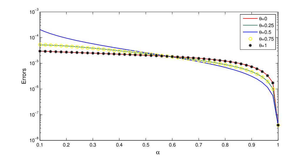
Table 1 reports the -norm of and the corresponding estimates of convergence rate for different values of , and the discretization step size . The table confirms the errors, for all the values of and shown, as goes to zero.
Example 2. (non-smooth solutions) In practice, due to the presence of the two-sided fractional derivative, the solution of (1) admits end-point singularities even if the source term is smooth. It was proved recently in [22] that, for , the leading singularity term takes the form when the diffusivity coefficient is constant. Similarly, one can show that leading singularity term takes the form , with presently, in the case of LS fractional derivative (), and the form , with presently, in the case of RS fractional derivatives (). For smooth , we conjecture the same singular behavior. Furthermore, we suggest that for , the leading singularity term has the generic form ( and ). However, demonstrating this point remains an open problem and it will be a subject of future work. Noting that, for and for , the authors in [12] studied the regularity properties of the solution of problem (1) where the fractional derivative operator is not of the Riemann-Liouville type, see (12, Equations (1.3) and (3.11)).
To support our claim, we choose now the source term such that is the exact solution of the problem with other settings as before. One can easily check that the truncation errors analyses provided above are not valid in this situation. We then apply to this problem our finite difference scheme for the LS () and RS () fractional derivatives cases for different values of and . Table 2 reports the discrete -norm of and estimates of the convergence rates . The results clearly indicate a convergence rate of the error in .
| 8 | 4.214e-02 | 0.2632 | 1.348e-02 | 0.5068 | 2.732e-03 | 0.7590 | |
|---|---|---|---|---|---|---|---|
| 9 | 3.527e-02 | 0.2567 | 9.510e-03 | 0.5037 | 1.618e-03 | 0.7556 | |
| 10 | 2.959e-02 | 0.2534 | 6.716e-03 | 0.5019 | 9.601e-04 | 0.7533 | |
| 11 | 2.485e-02 | 0.2517 | 4.745e-03 | 0.5010 | 5.702e-04 | 0.7518 | |
| 12 | 2.088e-02 | 0.2509 | 3.354e-03 | 0.5005 | 3.388e-04 | 0.7510 | |
| 8 | 4.145e-02 | 0.2399 | 1.336e-02 | 0.4940 | 2.692e-03 | 0.7402 | |
| 9 | 3.498e-02 | 0.2449 | 9.465e-03 | 0.4970 | 1.606e-03 | 0.7454 | |
| 10 | 2.946e-02 | 0.2475 | 6.700e-03 | 0.4985 | 9.562e-04 | 0.7478 | |
| 11 | 2.480e-02 | 0.2487 | 4.740e-03 | 0.4993 | 5.690e-04 | 0.7490 | |
| 12 | 2.086e-02 | 0.2494 | 3.352e-03 | 0.4996 | 3.384e-04 | 0.7495 | |
This degradation of the convergence rate was expected because the low regularity of the solution: . In the context of time-stepping schemes for fractional diffusion of fractional wave equations, adapted meshes with refinement (clustering of elements) around the singularity successfully improve the errors and consequently, the convergence rates, see [23, 25]. To check if such refinement approach could be useful in our problem of (steady) spatial fractional diffusion problem, we set (LS singularity) and consider a family of graded spatial meshes of based on a sequence of points given by , and is a refinement parameter. The objective is to refine the mesh at the boundary where the solution has a singularity. Table 3 reports the evolution with of the -norm of the error and estimated convergence rate and using , 3 and 4. The results show that one can obtain a convergence rate of the error that is . Finally, Fig. 3 compares the pointwise errors obtained for uniform and non-uniform meshes with when using the same number of discretization points , 512, 1024 and 2048. The reduction of the error due to the mesh refinement is clearly visible. Note that similar results can be obtained for using discretization points defined by to refine the mesh at the endpoint .
| 8 | 1.151e-02 | 0.4996 | 2.878e-03 | 0.7495 | 7.194e-04 | 0.9992 |
|---|---|---|---|---|---|---|
| 9 | 8.140e-03 | 0.4998 | 1.711e-03 | 0.7498 | 3.597e-04 | 0.9997 |
| 10 | 5.756e-03 | 0.4999 | 1.018e-03 | 0.7499 | 1.800e-04 | 0.9999 |
| 11 | 4.070e-03 | 0.4999 | 6.051e-04 | 0.7499 | 8.994e-05 | 0.9999 |
| 12 | 2.878e-03 | 0.5002 | 3.600e-04 | 0.7500 | 4.497e-05 | 0.9998 |

6 Concluding remarks
The objective of this work was to propose and analyze a finite-difference scheme for the solution of general one-dimensional fractional elliptic problems with a variable diffusion coefficient. For the proposed scheme, we proved the existence and uniqueness of the numerical solution and established the order of convergence for the truncation error with the spatial step size. Some numerical results were also presented for problems admitting both smooth and nonsmooth solutions.
This paper will form a stepping stone for the researchers who are interested in computational solutions of variable coefficient two-sided fractional derivative problems. The results obtained in this work lead to several questions that will have to be addressed in the future. First, it will crucial to address the reason(s) for the dramatic deterioration in the order of convergence of the finite difference scheme when the fractional order immediately departs from (classical case)? Second, it will be interesting to explore the possibility of incorporating the fractional exponent directly in the finite difference discretization, that is, fractionalizing the numerical scheme. A possible route along this direction could be inspired by the recent research papers on the fractionalization of the Crank-Nicolson time-scheme for solving time-fractional diffusion equation, see [9]. Finally, mechanisms for determining the order of singularity near the boundaries in the case of variable diffusivity remains to be developed. A possibility could be to look at series solution to (1). These and other related open questions will be the subject of future research.
References
- (1) D. Benson, S. W. Wheatcraft and M. M. Meerschaert, The fractional-order governing equation of Lévy motion, Water Resource Res., 36, 1413–1423, 2000.
- (2) C. Celik and M. Duman, Crank–Nicolson method for the fractional diffusion equation with the Riesz fractional derivative, J. Comput. Phys., 231, 1743–1750, 2012.
- (3) A.Chaves, Fractional diffusion equation to describe Lévy fights, Phys. Lett. A, 239, 12–16.
- (4) A.V.Chechkin, J.Klafter and I.M.Sokolov, Fractional Fokker–Planck equation for ultraslow kinetics, Europhys. Lett., 63, 326–332, 2003.
- (5) D. del-Castillo-Negrete, Chaotic transport in zonal flows in analogous geophysical and plasma systems, Phys. Plasmas, 7, 1702–1711, 2000.
- (6) D. del-Castillo-Negrete, B. A. Carreras and V. E. Lynch, Front dynamics in reactiondiffusion systems with Levy flights, Phys. Rev. Lett., 91, 018302, 2003.
- (7) W. Deng and J.S. Hesthaven, Local discontinuous Galerkin methods for fractional diffusion equations, ESAIM: Mathematical Modelling and Numerical Analysis, 47, 1845–1864, 2013
- (8) W. Deng, B. Li, W. Tian and P. Zhang, Boundary problems for the fractional and tempered fractional operatrors, https://arxiv.org/abs/1702.03639, 2018
- (9) Y. Dimitrov, Numerical approximations for fractional differential equations. J. Fract. Calc. Appl., 5(suppl. 3S):Paper no. 22, 1–45, 2014.
- (10) H. Ding, C. Li and Y. Chen, High–-order algorithms for Riesz derivative and their applications I, Abstract and Applied Analysis, 2014, 1–17, 2014.
- (11) V. J. Ervin and J. P. Roop, Variational formulation for the stationary fractional advection dispersion equation, Numer. Methods. Partial Differential Equations, 22, 559–576, 2006.
- (12) V. J. Ervin, N. Heuer and J. P. Roop, Regularity of the solution to 1D fractional order diffusion equations. Math. Comp., 2017, DOI: https://doi.org/10.1090/mcom/3295.
- (13) N. J. Ford, D. V. Savostyanov and N. L. Zamarashkin, On the Decay of the elements of inverse triangular Toeplitz matrices, SIAM J. Matrix Anal. Appl., 35, 1288–1302, 2014.
- (14) G. H. Hardy, Divergent Series, Clarendon Press, Oxford, 1949.
- (15) R. A. Horn and C. R. Johnson, Matrix Analysis, Cambridge University Press, New York, 2013.
- (16) B. Jin, R. Lazarov, J. Pasciak and W. Rundell, Variational formulation of problems involving fractional order differential operators, Math. Comput., 84, 2665–2700, 2015.
- (17) K. N. Le, W. McLean and K. Mustapha, Numerical solution of the time-fractional Fokker–Planck equation with general forcing, SIAM J. Numer. Anal., 54, 1763–1784, 2016.
- (18) E. Kharazmi, M. Zayernouri and G. Em Karniadakis, A Petrov-Galerkin Spectral Element Method for Fractional Elliptic Problems, https://arxiv.org/abs/1610.08608, 2016.
- (19) X. Li and C. Xu, The existence and uniqueness of the weak solution of the space-time fractional diffusion equation and a spectral method approximation, Commun. Comput. Phys., 8, 1016–1051, 2010.
- (20) Y. Liu, Y. Yan and M. Khan, Discontinuous Galerkin time stepping method for solving linear space fractional partial differential equations, Appl. Numer. Math., 115, 200–213, 2017.
- (21) V. Lynch, B. Carreras, D. del Castillo-Negrete, K. Ferreira-Mejias and H. Hicks, Numerical methods for the solution of partial differential equations of fractional order, J. Comput. Phys., 192, 406–421, 2003.
- (22) Z. Mao, S. Chen and J. Shen, Efficient and accurate spectral method using generalized Jacobi functions for solving Riesz fractional differential equations, Appl. Numer. Math., 106, 165–181, 2016.
- (23) W. McLean and K. Mustapha, A second-order accurate numerical method for a fractional wave equation, Numer. Math., 105, 481–510, 2007.
- (24) R. Metzler and J. Klafter, The random walk’s guide to anomalous diffusion: a fractional dynamics approach, Physics Reports, 339, 1–77, 2000.
- (25) K. Mustapha, An implicit finite difference time-stepping method for a sub-diffusion equation, with spatial discretization by finite elements, IMA J. Numer. Anal., 31. 719–739, 2011.
- (26) M. D. Ortigueira, Riesz potential operators and inverses via fractional centred derivatives, Int. J. Math. Mathematical Sci., 1–12, 2006.
- (27) I. Podlubny, Fractional Differential Equations, Academic Press, San Diego, 1999.
- (28) T. H. Solomon, E. R. Weeks and H. L. Swinney, Observation of anomalous diffusion and Lévy flights in a two-dimensional rotating flow, Phys. Rev. Lett., 71, 3975–3978, 1993.
- (29) E. Sousa, Finite difference approximations for a fractional advection diffusion problem, J. Comput. Phys., 228, 4038–4054, 2009.
- (30) M. Stynes and J. L. Gracia, A finite difference method for a two-point boundary value problem with a Caputo fractional derivative, IMA J. Numer. Anal., 35, 2015.
- (31) C. Tadjeran, M. M. Meerschaert and H.-P. Scheffler, A second-order accurate numerical approximation for the fractional diffusion equation, J. Comput. Phys., 205–213, 2006.
- (32) W. Tian, H. Zhou and W. Deng, A class of second order difference approximations for solving space fractional diffusion equations, Math. Comput., 84, 1703–1727, 2015.
- (33) H. Wang and D. Yang, Wellposedness of variable-coefficient conservative fractional elliptic differential equations, SIAM J. Numer. Anal., 51, 1088–1107, 2013.
- (34) H. Wang, D. Yang and S. Zhu, Inhomogeneous Dirichlet boundary-value problems of space-fractional diffusion equations and their finite element approximations, SIAM J. Numer. Anal., 52, 1292–1310, 2014.
- (35) H. Wang, D. Yang and S. Zhu, A Petrov-Galerkin finite element method for variable-coefficient fractional diffusion equations, Comput. Methods Appl. Mech. Engrg., 290, 45–56, 2015.
- (36) H. Zhang, F. Liu and V. Anh, Garlerkin finite element approximations of symmetric spacefractional partial differential equations, Appl. Math. Comput., 217, 2534–2545, 2010.
- (37) H. Zhou, W. Tian and W. Deng, Quasi–compact finite difference schemes for space fractional diffusion equations, J. Sci. Comput., 56, 45–66, 2013.