$M/G/c/c$ state dependent queuing model for a road traffic system of two sections in tandem

Nacira Guerouahane Email: naciraro@hotmail.fr Corresponding author: Corresponding author. Tel.: +213-34-21-08-00. Address: LaMOS Research Unit, Faculty of Exact Sciences, University of Bejaia, 06000 Bejaia, Algeria. Djamil Aissani Email: lamos_bejaia@hotmail.com Address: LaMOS Research Unit, Faculty of Exact Sciences, University of Bejaia, 06000 Bejaia, Algeria. Nadir Farhi Email: nadir.farhi@ifsttar.fr Address: Université Paris-Est, COSYS, GRETTIA, IFSTTAR, F-77447 Marne-la-Vallée, France. Louiza Bouallouche-Medjkoune Email: louiza_medjkoune@yahoo.fr Address: LaMOS Research Unit, Faculty of Exact Sciences, University of Bejaia, 06000 Bejaia, Algeria.

Abstract

We propose in this article a $M/G/c/c$ state dependent queuing model for road traffic flow. The model is based on finite capacity queuing theory which captures the stationary density-flow relationships. It is also inspired from the deterministic Godunov scheme for the road traffic simulation. We first present a reformulation of the existing linear case of $M/G/c/c$ state dependent model, in order to use flow rather than speed variables. We then extend this model in order to consider upstream traffic demand and downstream traffic supply. After that, we propose the model for two road sections in tandem where both sections influence each other. In order to deal with this mutual dependence, we solve an implicit system given by an algebraic equation. Finally, we derive some performance measures (throughput and expected travel time). A comparison with results predicted by the $M/G/c/c$ state dependent queuing networks shows that the model we propose here captures really the dynamics of the road traffic.

Keywords:

Traffic flow modeling , finite queuing systems ,

M/G/c/c

state dependent.

1 Introduction

Congestion is a phenomenon that arises in a variety of contexts. The most familiar representation is urban traffic congestion. Congested networks involve complex traffic interactions. Providing an analytical description of these intricate interactions is challenging. The dynamics of traffic flows is submitted to stochastic nature of traffic demand and supply functions of vehicles passing from one section to another.

One of the well known macroscopic traffic model on a road section is the LWR (Lighthill-Whitham-Richards) first-order continuum one [23, 26], which assumes the existence of a steady-state relationship for the traffic, called the fundamental diagram, giving the traffic flow in function of the vehicular density in the road section. In this paper, we present a reformulation of the $M/G/c/c$ state dependent queuing model [5] working with flows rather than speeds, and propose a stochastic traffic model based on this new formulation and inspired from the Godunov scheme [15, 22] of the LWR traffic model. We derive a stationary probability distribution of the $M/G/c/c$ state dependent queuing model on a road section, by considering density-flow fundamental diagrams rather than density-speed ones. The model assumes a quadratic fundamental diagram which correctly captures the stationary density-flow relationships in both non-congested and congestion conditions. By this, we consider the traffic demand and supply functions for the section, and distinguish three road section systems, an open road section, a constrained road section and a closed road section. Finally, we present a model of two road sections in tandem, derive some performance measures and show on an academic example that the model captures the dynamics of the road traffic. The model we present here can be used to the analysis of travel times through road traffic networks (derive probability distributions, reliability indexes, etc), as in [9, 10, 11], where an algebraic deterministic approach is used. The approach present here remains also valid with a triangular fundamental diagram (which is the most used), but the formulas will change [14].

The remainder of this article is organized as follows. In Section 2, we first present a review of the existing works. In this regard, we present in Section 3 a short review of the $M/G/c/c$ state dependent queuing model of Jain and Smith [27]. We then propose a new reformulation of this model by working with flows rather than speeds. We rewrite the stationary probability distribution of the number of cars on the road section. In Section 4, we present a model of two road sections in tandem where both road sections influence each other. An implicit system given by an algebraic equation is solved, in order to deal with this mutual dependence. We derive some performance measures of both road sections (throughput and expected travel time) and compare our simulation results with those of existing $M/G/c/c$ state dependent queuing models (Kerbache and Smith model). In Section 5, we briefly summarize our findings and future work.

2 Literature review

Congestion is a phenomenon that arises on local as well as large areas, whenever traffic demand exceeds traffic supply. Traffic flow on freeways is a complex process with many interacting components and random perturbations such as traffic jams, stop-and-go waves, hysteresis phenomena, etc. These perturbations propagate from downstream to upstream sections. During traffic jams, drivers are slowing down when they observe traffic congestion in the downstream section, causing upstream propagation of a traffic density perturbation. A link of the network is modeled as a sequence of road sections, for which fundamental diagrams are given. As the sequence of sections is in series, if any section is not performing optimally, the whole link will not be operating efficiently. We base here on the LWR first order model [23, 26], for which numerical schemes have been performed since decades [8, 15, 22]. In the Godunov scheme [22], as well as in the cell transmission model (CTM) [8], traffic demand and supply functions are defined and used. The demand-supply framework provides a comprehensive foundation for the LWR first order node models. Flow interactions in these models result from limited inflow capacities of the downstream links. Recently, in [28] framework has been supplemented with richer features such as conflicts within the node. In [25], a dynamic network loading model that yields queue length distributions was presented. This model is a discretized, stochastic instance of the kinematic wave model (KWM). In [4], the compositional stochastic model extends the cell transmission model [8] by defining demand and supply functions explicitly as random variables, and describing how speed evolves dynamically in each link of the road network. Several simulation models based on queueing theory have been developed, but few studies have explored the potential of the queueing theory framework to develop analytical traffic models. The development of analytical, differentiable, and computationally tractable probabilistic traffic models is of wide interest for traffic management. The most common approach is the development of analytical stationary models [25]. A review of stationary queueing models for highway traffic and exact analytical stationary queueing models of unsignalized intersections is given in deferent literatures [17, 29, 30]. In [1, 13, 16], the authors contributed to the study of signalized intersections and presented a unifying approach to both signalized and unsignalized intersections. These approaches resort to infinite capacity queues, and thus fail to account for the occurrence of breakdown and their effects on upstream links. Modeling and calculating traffic flow breakdown probability remains an important issue when analyzing the stability and reliability of transportation system [3, 31].

Finite capacity queueing theory imposes a finite upper bound on the length of a queue. This allows to account for finite link lengths, which enables the modeling and analysis of breakdowns. Finite capacity queueing network (FCQN) model are of interest for a variety of applications such as the study of hospital patient flow, manufacturing networks, software architecture networks, circulation systems, prison networks [5], etc. The methods in [2, 5, 27] resort to finite capacity queueing theory and derive stationary performance measures. The stationary distribution of finite capacity queueing network exist only for networks with two or three queues with specific topologies [12, 20, 21]. An analytic queueing network model that preserves the finite capacity for two queues, under a set of service rate scenarios proposed in [24].

For more general networks, approximation methods are used to evaluate the stationary distributions, and the General Expansion Method (GEM) was developed [18, 19]. The GEM characterized by an artificial holding node, which is added and preceded each finite queue in the network in order to register all blocked cars caused by the downstream section. The interested reader may check details in [19]. In [6], the authors describe a methodology for approximate analysis of open state dependent $M/G/c/c$ queueing networks, and a system of two queues in tandem topology was analyzed. The evacuation problem was analyzed using $M/G/c/c$ state dependent queuing networks in [7] when an algorithm was proposed to optimize the stairwell case and increase evacuation times towards the upper stories. In [14], the authors present another version of $M/G/c/c$ state dependent queuing model, where a triangular fundamental diagram is considered, which leads to apply the demand and supply functions in order to analyze a system of two queues in tandem topology.

3 Review on the M/G/c/c state dependent queuing model

In this section, we present the $M/G/c/c$ state dependent queuing model [5, 27]. A link of a road network is modeled with $c$ servers set in parallel, where $c$ is the maximum number of cars that can move on the road (density-like). The car-speed is assumed to be dependent on the number of cars $n$ on the road, according to a non-increasing density-speed relationship. Two cases of speed are considered, linear and exponential. In the linear case, we have

v_{n}=v_{1}\left(\frac{c-n+1}{c}\right),

(1)

where $v_{i}$ is the speed corresponding to $i$ cars moving on the road, and $v_{1}$ is the free flow speed. In the exponential case, we have

v_{n}=v_{1}\exp\left[-\left(\frac{n-1}{\beta}\right)^{\gamma}\right],

(2)

in which $\beta$ and $\gamma$ are shape and scale parameters respectively.

\begin{array}[]{ll}\beta&=\frac{a-1}{[\ln(v_{1}/v_{a})]^{1/\gamma}}=\frac{b-1}{[\ln(v_{1}/v_{b})]^{1/\gamma}}.\\ &\\ \gamma&=\ln[\frac{\ln(v_{a}/v_{1})}{\ln(v_{b}/v_{1})}]/\ln(\frac{a-1}{b-1}).\end{array}

The values $a$ and $b$ are arbitrary points, used to adjust the exponential curve [5, 27]. The arrival process of cars into the link is assumed to be Poisson with rate $\lambda$ , while the service rate of the $c$ servers depend on the number $n$ of cars on the road. A normalized service rate $f(n)$ is considered, and is taken $f(n)=v_{n}/v_{1}\leq 1$ . In the linear case, we have $f(n)=(c-n+1)/c$ . In the exponential case, we have $f(n)=\exp[-((n-1)/\beta)^{\gamma}]$ . We notice here that $v_{1}$ is the speed corresponding to one car in the road (ie. the free speed).

The stationary probability distribution $P_{n}=Prob\penalty\ (N=n)$ of the number of cars $N$ in the $M/G/c/c$ state dependent model have been developed and shown in [5] to be stochastic equivalent to $M/M/c/c$ queueing model. Therefore, these probabilities can be written as follows.

P_{n}=\frac{(\lambda L/v_{1})^{n}}{\prod_{i=1}^{n}if(i)}P_{0},\qquad P_{0}=\left(1+\sum_{n=1}^{c}\frac{(\lambda L/v_{1})^{n}}{\prod_{i=1}^{n}if(i)}\right)^{-1},\quad n=1,...,c.

(3)

where $L$ is the length of the road section.

From $P_{n}$ , other important performance measures can be easily derived.

1.

The blocking probability : $P_{c}=P_{0}(\lambda L/v_{1})^{c}/\prod_{i=1}^{c}if(i).$
2.

The throughput : $\theta=\lambda(1-P_{c}).$
3.

The expected number of cars in the section : $\bar{N}=\sum_{n=1}^{c}nP_{n}.$
4.

The expected service time : $W=\bar{N}/\theta.$

In the following section, we rewrite the model presented in this section, by considering a car density-flow relationship rather than a density-speed one. This reformulation permits us to consider demand and supply functions which model limit conditions for car-traffic, and by that, to model two road sections in tandem, in Section 4.

3.1 Reformulation of the M/G/c/c state dependent model

In this section, we first reformulate the $M/G/c/c$ state dependent model of Jain and Smith, by considering car-flows rather than car-speeds. Indeed, the linear case of that model considers a linear relationship of the speed as a function of the car-density. This is equivalent to considering a quadratic relationship of the car-flow as a function of the car-density; see Figure 1. It is easy to check that this quadratic relationship is written as follows.

q_{n}=q_{\max}\left(1-\left(\frac{c-2n+1}{c+1}\right)^{2}\right).

(4)

Indeed, one can for example verify that parting from (4), we retrieve (1)

\frac{v_{n}}{v_{1}}:=\frac{q_{n}/\rho_{n}}{q_{1}/\rho_{1}}=\frac{c-n+1}{c},

where $\rho_{n}=n/L$ .

Refer to caption — Figure 1: In the left side, the car-density - speed relationship. In the right side, the corresponding car-density - flow relationship.

The stationary probabilities (3) are then rewritten as follows.

P_{n}=\frac{(\lambda/q_{\max})^{n}}{\prod_{i=1}^{n}ig(i)}P_{0},\qquad P_{0}=\left(1+\sum_{n=1}^{c}\frac{(\lambda/q_{\max})^{n}}{\prod_{i=1}^{n}ig(i)}\right)^{-1},\quad n=1,...,c.

(5)

where

g(i)=\frac{q_{i}/q_{\max}}{i}.

The objective of working with flows rather than speeds here is to consider the demand and supply functions which we will use in the following sections, for the model of two road-sections in tandem. From (1) and (4), the relationship between the free speed $v_{1}$ and the maximum car-flow $q_{\max}$ is given as follows.

q_{\max}=v_{(\frac{c+1}{2})}\rho_{(\frac{c+1}{2})}=\frac{v_{1}}{Lc}\left(\frac{c+1}{2}\right)^{2}.

(6)

The demand $\Delta_{n}$ and the supply $\Sigma_{n}$ functions are given as follows.

\Delta_{n}=\begin{cases}q_{n}&\text{if}\penalty\ \penalty\ 0\leq n\leq\frac{c+1}{2},\\ q_{\max}&\text{if}\penalty\ \penalty\ \frac{c+1}{2}<n\leq c+1.\end{cases}

(7)

\Sigma_{n}=\begin{cases}q_{\max}&\text{if}\penalty\ \penalty\ 0\leq n\leq\frac{c+1}{2},\\ q_{n}&\text{if}\penalty\ \penalty\ \frac{c+1}{2}<n\leq c+1.\end{cases}

(8)

Demand and supply diagrams are shown in Figure 2, where the parameters of Table 1 are considered.

In the following section, we consider three configuration models of a road section: open, constrained and closed road section. We will explain the role of each model, and tell how these models will be used for the model of two sections in tandem.

3.2 Open, constrained and closed road sections

We distinguish here three road section systems.

1.

An open road section is a road section where the traffic out-flow from the section is only constrained by the traffic demand of the section, given in function of the number of cars in the section. It is equivalent to the traffic system presented above in Section 3.1, where the traffic fundamental diagram is restrained to only its traffic demand part (ie with infinite traffic supply). In such a road section, which we index by $i$ , if we denote by $\Delta_{i}$ and $\Sigma_{i}$ the traffic demand and supply of the section (induced by the car-density of the section) respectively, and $q_{out}$ the outflow from the section, then we have (see Figure 3)

$q_{out}=\Delta_{i}.$ (9)
2.

A constrained road section is a road section out flowing to another downstream section, and where the outflow of the considered road section is constrained by the traffic demand of that section, and by the traffic supply of the downstream section. If we index the downstream section by the index $i+1$ , denote by $\Sigma_{i+1}$ the traffic supply of the downstream section, and consider the same notations used above, then we have (see Figure 3)

$q_{out}=\min(\Delta_{i},\Sigma_{i+1}).$ (10)
3.

A closed road section is the road section system presented above in Section 3.1, for which the outflow is given by the fundamental traffic diagram with both demand and supply parts, and where both the parts are constrained by the car-density of the section. Using the same notation as above, the out-flow from the section is given as follows (see Figure 3)

$q_{out}=\min(\Delta_{i},\Sigma_{i}).$ (11)

Basing on the three systems presented above, we present in the following section, a model of two road sections in tandem. It is a kind of a constrained section where the downstream section is a closed one.

4 Two road sections in tandem

We propose in this section a state-dependent $M/G/c/c$ model for two road sections in tandem. The whole system is a concatenation of two road sections: a $M/G/c/c$ state dependent constrained section (section 1), with an $M/G/c/c$ state dependent closed section (section 2); see Figure 4. Since the downstream section (section 2) is a closed one, which corresponds to the traffic system presented in Section 3.1, the supply flow of section 2 is stochastic, and is given in function of the probability distribution of the number of cars in section 2.

We assume quadratic flow-density fundamental diagrams for the two sections. The car-flow outgoing from section 1 and entering to section 2 ( $q_{12}(n_{1},n_{2})$ ) is given by the minimum between the traffic demand on section 1 and the traffic supply of section 2.

q_{12}(n_{1},n_{2})=\min(\Delta_{1}(n_{1}),\Sigma_{2}(n_{2})).

(12)

The car-flow outgoing from section 2, and also from the whole system is denoted by $q_{2}$ . The objective here is to determine the stationary probability distributions $P^{(1)}$ and $P^{(2)}$ of the number of cars in section 1 and section 2 respectively, as well as the stationary probability distribution $P^{(1,2)}$ of the couple $(n_{1},n_{2})$ of numbers of cars in sections 1 and 2 respectively.

We notice here that this cannot be calculated directly since both road sections influence each other. Indeed, $P^{(2)}$ depends on $q_{12}$ which depends on the traffic demand of section 1. Similarly, $P^{(1)}$ depends on the traffic supply of section 2, since section 1 is constrained by section 2. We propose below an iterative approach for the calculus of such probabilities.

4.1 The model

The procedure we propose here for the determination of $P^{(1)},P^{(2)}$ and $P^{(1,2)}$ consists in solving an implicit system given by an algebraic equation, in order to deal with the mutual dependence between sections 1 and 2. We denote by $\theta$ the average outflow from section 1 (average of $q_{12}$ ), which is also the average inflow to section 2; and by $\delta$ the average outflow from section 2 (average of $q_{2}$ ), which is the average outflow of the whole system.

We notice that if $\theta$ is known, then the probability distributions $P^{(1)},P^{(2)}$ and $P^{(1,2)}$ can be obtained in function of $\theta$ . Indeed, section 2 being a $M/G/c/c$ state dependent closed section with an average arrival flow $\theta$ , $P^{(2)}$ can be obtained in function of $\theta$ . After that, section 1 being constrained by the supply of section 2 (with known $P^{(2)}$ ), $P^{(1,2)}$ and then $P^{(1)}$ can be obtained in function of $P^{(2)}$ and thus in function of $\theta$ . Moreover, from $P^{(1)}$ we can obtain $q_{12}$ in function of $\theta$ , and then the expectation of $q_{12}$ gives $\theta$ in function of itself.

From the latter remark, we propose the following iterative algorithm for the calculus of $\theta$ and of the probabilities $P^{(1)},P^{(2)}$ and $P^{(1,2)}$ .

Step $0$ . Initialize $\theta=\theta_{0}$ .
Step $k$ (for $k\geq 1$ ).

(1)

$P^{(2)}$ is obtained in function of $\theta=\theta_{k-1}$ .
Section 2 is a $M/G/c/c$ state dependent closed section, with an average arrival flow $\theta$ , which is unknown. According to (5), the stationary probability distribution of the number $n_{2}$ of cars on section 2 is given, in function of $\theta$ , as follows.

\begin{array}[]{ll}P^{(2)}_{n_{2}}(\theta)&=\frac{(\theta/q_{\max_{2}})^{n_{2}}}{\prod_{i=1}^{n_{2}}ig_{2}(i)}P^{(2)}_{0}(\theta),\qquad n_{2}=1,...,c_{2}.\\ \\ P^{(2)}_{0}(\theta)&=\left(1+\sum_{n_{2}=1}^{c_{2}}\frac{(\theta/q_{\max_{2}})^{n_{2}}}{\prod_{i=1}^{n_{2}}ig_{2}(i)}\right)^{-1}.\end{array}

(13)

where

g_{2}(i)=\frac{q_{2}(i)/q_{\max_{2}}}{i}.

(2)

$P^{(1,2)}$ and then $P^{(1)}$ are obtained from $\lambda$ and $P^{(2)}$ , and thus in function of $\theta=\theta_{k-1}$ .
Section 1 is constrained by the supply of section 2. As the normalized service rate $g_{1}(i_{1},i_{2})$ of section 1 depends on the number of cars on section 2, which itself depends on $\theta$ , the stationary probability distribution $P^{(1)}$ of the number of cars in section 1, is also given in function of $\theta$ . The normalized service rate $g_{1}(i_{1},i_{2})$ of section 1 is given as follows.

g_{1}(i_{1},i_{2})=\frac{q_{12}/q_{\max_{1}}}{i_{1}}=\frac{\min(\Delta_{1}(i_{1}),\Sigma_{2}(i_{2}))/q_{\max_{1}}}{i_{1}}.

(14)

In order to write $P^{(1)}$ , let us first write the stationary probability distribution of the number of cars on section 1, conditioned by the number of cars on section 2, which we denote by $P^{(1\mid 2)}$ , and which is independent of $\theta$ .

\begin{array}[]{ll}P^{(1\mid 2)}_{(n_{1}\mid n_{2})}(\lambda)&=Prob\penalty\ (N_{1}=n_{1}\mid N_{2}=n_{2})=\frac{(\lambda/q_{\max_{1}})^{n_{1}}}{\prod_{i=1}^{n_{1}}ig_{1}(i_{1},n_{2})}P^{(1\mid 2)}_{(0\mid n_{2})}(\lambda),\\ \\ P^{(1\mid 2)}_{(0\mid n_{2})}(\lambda)&=Prob\penalty\ (N_{1}=0\mid N_{2}=n_{2})=\left(1+\sum_{n_{1}=1}^{c_{1}}\frac{(\lambda/q_{\max_{1}})^{n_{1}}}{\prod_{i=1}^{n_{1}}ig_{1}(i_{1},n_{2})}\right)^{-1}.\end{array}

(15)

Thus, the stationary probability distribution $P^{(1)}$ of the number of cars in section 1, which depends on $\lambda$ and $\theta$ , is given as follows.

\begin{array}[]{ll}P^{(1)}_{n_{1}}(\lambda,\theta)&=\sum_{n_{2}=1}^{c_{2}}P^{(1\mid 2)}_{(n_{1}\mid n_{2})}(\lambda)P^{(2)}_{n_{2}}(\theta),\\ \\ P^{(1)}_{0}(\lambda,\theta)&=\sum_{n_{2}=1}^{c_{2}}P^{(1\mid 2)}_{(0\mid n_{2})}(\lambda)P^{(2)}_{n_{2}}(\theta).\end{array}

(16)

(3)

$q_{12}$ is obtained from $P^{(1)}$ , and in function of $\theta=\theta_{k}$ , and finally $\theta_{k+1}=\mathbb{E}(q_{12}(\theta_{k}))$ .
The average outflow from section 1, $\theta$ , is given in function of $P^{(1)}$ as follows.

$\theta_{k}=\lambda\left(1-P^{(1)}_{c_{1}}(\lambda,\theta_{k-1})\right).$ (17)

The procedure consists then in solving the following implicit equation on the scalar $\theta$ .

\theta=\lambda\left(1-P^{(1)}_{c_{1}}(\lambda,\theta)\right).

(18)

The solution of that equation, if it exists, and if it is unique, gives the value of the asymptotic average flow passing from section 1 to section 2, and by that, the stationary probability distributions $P^{(2)},P^{(1\mid 2)}$ and $P^{(1)}$ . The stationary probability distribution $P^{(1,2)}$ can be easily deduced from $P^{(1\mid 2)}$ and $P^{(2)}$ . We notice here that equation (18) is a fixed-point-like equation.

In the following section, we give some results on the fixed-point equation solving.

4.2 Fixed-point equation solving

We use the following notations.

1.

$h(\theta)=\lambda\left(1-P^{(1)}_{c_{1}}(\lambda,\theta)\right)$ ,
2.

$e(\theta)=h(\theta)-\theta$ .

Equation (18) is written $\theta=h(\theta)$ , and it is equivalent to $e(\theta)=0$ .

Below, we give some results on the resolution of equation (18).

Theorem 4.1.

A solution for equation (18) exists and is unique.

Proof.

See A.

The following result gives a condition on the couple $(\lambda,\theta)$ , under which the sequence $\theta_{k},k\in\mathbb{N}$ defined by fixed point iteration (17) (i.e. $\theta_{k}=h(\theta_{k-1}))$ converges for every initial value $\theta_{0}\in[0,\lambda]$ .

Theorem 4.2.

If $\exists\varepsilon>0$ such that $\varepsilon<\theta/\lambda$ , and if

\sum_{n_{2}=1}^{c_{2}}P^{(1\mid 2)}_{c_{1}\mid n_{2}}(\lambda)P^{(2)}_{n_{2}}(\theta)\left(n_{2}-\sum_{k_{2}=1}^{c_{2}}k_{2}P^{(2)}_{k_{2}}(\theta)\right)\leq\varepsilon,

then the fixed point iteration converges to the unique fixed point of the fixed point equation.

Proof.

See B.

We do not have other explicit formulas than the condition of Theorem 4.2. We know that for low values of $\lambda$ , we have $-1<d\;h(\theta)/d\theta\leq 0,\forall\theta\in[0,\lambda]$ , and the iteration of the fixed point equation converges, independently of the initial value of $\theta$ , to the unique fixed point. However, we also know that for high values of $\lambda$ , there exists an interval $(\theta_{1},\theta_{2})$ where $d\;h(\theta)/d\theta<-1$ . In such cases, the fixed point is unstable. Nevertheless, the sequence $\theta_{k},k\in\mathbb{N}$ oscillates between two adherence values $h(0)=\lambda$ and $h(\lambda)$ , giving $(\lambda+h(\lambda))/2$ as the asymptotic average value of $\theta$ , see Figures 5 and 6.

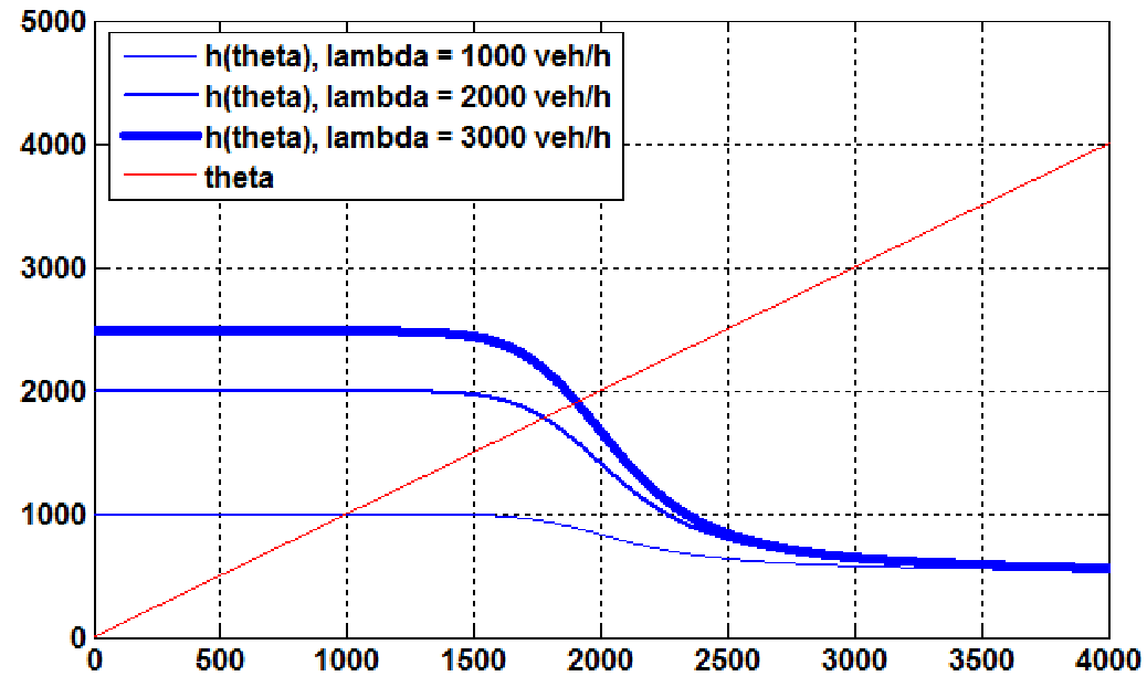
In Figure 5, we give in blue color the function $h(\theta)$ for different values of $\lambda$ . The red line is the first bisector. The fixed point verifying $h(\theta)=\theta$ is then the intersection of the blue curve with the red one. We see in this figure that the derivative of $h(\theta)$ with respect to $\theta$ on the fixed point is decreasing with $\lambda$ , starting from zero. Indeed, for low values of $\lambda$ , we have $dh(\theta)/\theta=0$ . As $\lambda$ increases, $dh(\theta)/\theta$ decreases. As explained above, while $dh(\theta)/\theta>-1$ , we know that the fixed point is stable. However, once $dh(\theta)/\theta>-1$ , the fixed point is unstable.

Figure 6 illustrates the two cases of stable and unstable fixed points, depending on the value of $\lambda$ . In the first case (left side of the figure), we have $\lambda=2000$ veh/h; see also Figure 5. In this case, the fixed point is stable, and the iteration converges to it. In the second case (right side of Figure 6), we have $\lambda=3000$ veh/h; see also Figure 5. In this case, the fixed point is unstable, and the iteration oscillates from the two values $h(0)=\lambda$ and $h(\lambda)$ .

In the following section, we explain how to compute the stationary probability distributions in function of the average flow $\theta$ , calculated by the fixed point iteration.

4.3 The stationary probability distributions

Once $\theta$ is obtained, the whole stationary regime of the system of two road sections in tandem is determined. Indeed, the stationary probability distributions $P^{(1)},P^{(2)}$ and $P^{(1|2)}$ are given by (16), (13) and (15) respectively. The stationary joint probability distribution $P^{(1,2)}$ of the couple $(n_{1},n_{2})$ of the number of cars in sections 1 and 2 respectively, is then easily deduced.

P^{(1,2)}_{(n_{1},n_{2})}=P^{(1|2)}_{n_{1}|n_{2}}P^{(2)}_{n_{2}},\quad\forall 0\leq n_{1}\leq c_{1},0\leq n_{2}\leq c_{2}.

In the following, we illustrate those probability distributions for given parameters of the system. Table 1 gives the fixed parameters for the illustrations, where $L$ , $v_{1}$ , $\rho_{j}$ and $q_{\max}$ denote respectively section length, free speed, jam-density and maximum car-flow.

Table 1: Parameters for sections 1 and 2.

Section $i$ $L$ (km) $v_{1}$ (km/h) $\rho_{j}$ (veh/km) $q_{\max}$ (veh/h) 1 0.1 100 180 5000 2 0.1 50 180 2500

Let us notice that $\rho_{cr}=\rho_{j}/2$ (quadratic fundamental diagram), and $c=L\rho_{j}$ .
$\rho_{cr}$ and $c$ denote respectively critical car-density and road section capacity in term of maximum number of cars.

Figure 7 compares the stationary distribution probability of the two following cases.

1.

One closed road section (Jain and Smith model), with parameters of section 2 in Table 1. (Blue color in Figure 7).
2.

One constrained road section, with parameters of section 1 in Table 1. The section is assumed to be constrained by a closed road section whose parameters are those of section 2 in Table 1. (Red color in Figure 7).

The average car inflow $\lambda$ is varied from one illustration to another in Figure 7.

We notice here that the constrained road has a maximum flow capacity of $5000$ veh/h, but it is constrained by a closed road with a maximum flow capacity of $2500$ veh/h. We remark from Figure 7, that the constrained section is more likely to be congested than the closed one, even though a priori they are both constrained by a maximum flow capacity of $2500$ veh/h.

Figure 8 gives the stationary probability distributions $P^{(1,2)}$ of the couple $(n_{1},n_{2})$ of numbers of cars in sections 1 and 2 respectively. The average arrival rate $\lambda$ is varied from one illustration to another. Parameters of Table 1 are used. $\lambda$ takes the values of $1000$ veh/h, $2000$ veh/h, $2500$ veh/h and $3000$ veh/h.

In Figure 9, we give the throughputs of sections 1 and 2 in the case where the two sections are set in tandem. The throughput $\theta$ of section 1 is given by (18), and it is the solution of the fixed point iteration. The throughput $\delta$ (see 4) is computed by the same way (Little’s law), once $\theta$ is determined.

\delta=\theta\left(1-P^{(2)}_{c_{2}}(\theta)\right).

Figure 9 displays for an increasing arrival rate, $\lambda$ , the throughput through sections 1 and 2 of the whole system of two road sections in tandem. The parameters of each road section are those given in Table 1. We remark from Figure 9, that throughput through the sections 1 and 2 is equal to the arrival rate $\lambda$ up to roughly $2200$ veh/h. This comes directly from the fact that the capacities are not restrictive. However, the trend changes at about $2300$ veh/h (well below $2500$ veh/h), and the throughput does not increase anymore.

4.4 Performance measures of two sections in tandem topology

We consider the system of two sections in tandem topology presented in Figure 4, with parameters of Table 1. The bottleneck in section 2 is most difficult to be analyzed because of the mutual dependence between the two sections set in tandem. In the next, we compare the throughput and the expected service time of our method with the method of Kerbache and Smith [19].

Figure 10 compares the throughputs of sections 1 and 2 of our method with the expansion method of Kerbache and Smith (open $M/G/c/c$ state dependent queueing networks) [19].

We remark from Figure 10, that when the arrival rate $\lambda$ is low, our throughputs ( $\theta$ of section 1 and $\sigma$ of section 2) are similar to the throughputs of the expansion method of Kerbache and Smith. In this case, the arrival rate is very light and easily accepted by section 2 without any blocking. When the arrival rate $\lambda$ is large, our throughputs is low as compared to the throughputs of $M/G/c/c$ state dependent queueing networks, because the constrained section (section 1 of our model ) is more likely to be congested than the open section (section 1 in the expansion method of Kerbache and Smith).

Using Little’s Law, Figure 11 compares the expected service time of sections 1 and 2 of our method with the one of method of Kerbache and Smith [19]. We remark here that under a light arrival rate $\lambda$ , the expected service time almost corresponds to the free service time $(L/v_{1})$ . Under a heavy arrival rate, vehicles slow down and the expected service time increases in value for the two models. Our expected travel time remains near the upper bound of the expansion method of Kerbache and Smith.

5 Conclusion and future work

In this paper, we have presented a queuing model for road traffic that preserves the finite capacity property of the real system. Based on the $M/G/c/c$ state dependent queuing model, we have proposed a stochastic queuing model for the road traffic which captures the stationary density-flow relationship in both uncongested and congestion conditions. First results of the proposed model are presented. A comparison with results predicted by the classical $M/G/c/c$ state dependent queuing model shows that the proposed model correctly captures the interaction between upstream traffic demand and downstream traffic supply. Future work shall derive more analytic results on the proposed model, and include the extension of the model to complicated tree-topologies (complex series, merge, and split networks). Another interesting extension is the treatment of the case where the arrival rate follow a general distribution (general state dependent queuing model). The case where traffic demand, traffic supply and fundamental diagrams are stochastic will also be treated.

Acknowledgements

The authors wish to thank the editor-in-chief, and the anonymous reviewers whose constructive suggestions helped improve this paper.

Appendix A Proof of Theorem 4.1

1.
Existence. We have $e:[0,\lambda]\to[0,\lambda]$ .
- (a)
  
  $e(0)=h(0)=\lambda(1-P^{(1)}_{c_{1}}(\lambda,0))=\lambda\left(1-\sum_{n_{2}=1}^{c_{2}}P^{(1\mid 2)}_{(c_{1}\mid n_{2})}(\lambda)P^{(2)}_{n_{2}}(0)\right)$ .
  $P^{(2)}_{n_{2}}(0)=0,\forall n_{2}\neq 0$ and $P^{(2)}_{0}=1$ .
  Therefore, $e(0)=\lambda(1-P^{(1\mid 2)}_{(c_{1}\mid 0)}(\lambda))>0$
  since $P^{(1\mid 2)}_{(c_{1}\mid 0)}(\lambda)<1$ , because $P^{(1\mid 2)}_{(0\mid 0)}(\lambda)>0$ and $\lambda>0$ .
- (b)
  
  $e(\lambda)=h(\lambda)-\lambda=\lambda(1-P^{(1)}_{c_{1}}(\lambda))-\lambda=-\lambda P^{(1)}_{c_{1}}(\lambda)<0$
  since $P^{(1)}_{c_{1}}(\lambda)>0$ and $\lambda>0$ .
Using the theorem of intermediate values, $e$ is continuous from $[0,\lambda]$ into $[0,\lambda]$ , and we have $e(0)>0$ and $e(\lambda)<0$ . We conclude that $\exists\theta\in[0,\lambda]$ such that $e(\theta)=0$ .

Uniqueness. For the uniqueness of the fixed point, it is sufficient to show that $e$ is decreasing in $[0,\lambda]$ . Let us calculate $d\;e(\theta)/d\theta$ .

\frac{d\;e(\theta)}{d\theta}=\frac{d\left(\lambda-\lambda\sum_{n_{2}=1}^{c_{2}}P^{(1\mid 2)}_{(c_{1}\mid n_{2})}(\lambda)P^{(2)}_{n_{2}}(\theta)-\theta\right)}{d\theta}.

One can easily show that

\frac{dP^{(2)}_{n_{2}}}{d\theta}=\frac{1}{\theta}P^{(2)}_{n_{2}}(\theta)\left(n_{2}-\bar{n}_{2}(\theta)\right),

where

\bar{n}_{2}(\theta)=\mathbb{E}_{P^{(2)}}(n_{2})=\sum_{k_{2}=1}^{c_{2}}k_{2}P^{(2)}_{k_{2}}(\theta).

Then

\frac{d\;e(\theta)}{d\theta}=-\frac{\lambda}{\theta}\sum_{n_{2}=1}^{c_{2}}P^{(1\mid 2)}_{c_{1}\mid n_{2}}(\lambda)P^{(2)}_{n_{2}}(n_{2}-\bar{n}_{2}(\theta))\;-1.

Let us show that

S\stackrel{{\scriptstyle def}}{{=}}\sum_{n_{2}=1}^{c_{2}}P^{(1\mid 2)}_{c_{1}\mid n_{2}}(\lambda)P^{(2)}_{n_{2}}(\theta)(n_{2}-\bar{n}_{2}(\theta))\geq 0.

(19)

We have $P^{(1\mid 2)}_{c_{1}\mid n_{2}}(\lambda)$ is increasing with respect to $n_{2}$ ; see (14) and (15).

Let $n^{*}_{2}=n^{*}_{2}(\theta)$ be defined as follows $n^{*}_{2}=\max\{n_{2}\leq c_{2},n_{2}-\bar{n}_{2}(\theta)<0\}$ . Then

\begin{array}[]{ll}S&=\sum_{n_{2}=1}^{n^{*}_{2}}P^{(1\mid 2)}_{c_{1}\mid n_{2}}(\lambda)P^{(2)}_{n_{2}}(\theta)(n_{2}-\bar{n}_{2}(\theta))+\sum_{n_{2}=n^{*}_{2}}^{c_{2}}P^{(1\mid 2)}_{c_{1}\mid n_{2}}(\lambda)P^{(2)}_{n_{2}}(\theta)(n_{2}-\bar{n}_{2}(\theta))\\ \\ &\geq\sum_{n_{2}=1}^{n^{*}_{2}}P^{(1\mid 2)}_{c_{1}\mid n^{*}_{2}}(\lambda)P^{(2)}_{n_{2}}(\theta)(n_{2}-\bar{n}_{2}(\theta))+\sum_{n_{2}=n^{*}_{2}}^{c_{2}}P^{(1\mid 2)}_{c_{1}\mid n^{*}_{2}}(\lambda)P^{(2)}_{n_{2}}(\theta)(n_{2}-\bar{n}_{2}(\theta))\\ \\ &=P^{(1\mid 2)}_{c_{1}\mid n^{*}_{2}}(\lambda)\sum_{n_{2}=1}^{c_{2}}P^{(2)}_{n_{2}}(\theta)(n_{2}-\bar{n}_{2}(\theta))=0.\end{array}

Hence $d\;e(\theta)/d\theta<0$ , and the fixed point is unique.

∎

Appendix B Proof of Theorem 4.2

Following the proof of Theorem 4.1 ( A), we have

\frac{d\;h(\theta)}{d\theta}=\frac{d\;e(\theta)}{d\theta}+1=-\frac{\lambda}{\theta}S,

where $S$ is given by (19) in the proof of Theorem 4.1.

The condition of Theorem 4.2 can be written $\exists 0\leq\varepsilon<\theta/\lambda$ such that $S\leq\varepsilon$ . Therefore, if this condition is satisfied, then $\exists 0\leq\eta<1$ such that $d\;h(\theta)/d\theta>-1$ .

Then since we have already shown in the proof of Theorem 4.1 ( A) that $s\geq 0$ , and by that, $d\;h(\theta)/d\theta\leq 0$ , then, under the condition of Theorem 4.2, we have $0\leq d\;h(\theta)/d\theta<1$ .

Hence the fixed point iteration converges to the unique fixed point of the fixed point equation.

∎

References

[1] Balsamo S, Donatiello L. On the cycle time distribution in a two-stage cyclic network with blocking. IEEE Transactions on Software Engineering 1989; 15(10):1206–1216.
[2] Bedell P, MacGregor Smith J. Topological arrangements of m/g/c/k, m/g/c/c queues in transportation and material handling systems. Computers and Operations Research 2012; 39:2800-2819.
[3] Brilon W, Regler M. Reliability of freeway traffic flow: a stochastic concept of capacity. In: Proceedings of 16th International Symposium of Transportation and Traffic Theory. College Park, Maryland; 2005.
[4] Boel R, Mihaylova L. A compositional stochastic model for real time freeway traffic simulation. Transportation Research Part B 2006; 40:319-334.
[5] Cheah JY, MacGregor Smith J. Generalized M/G/C/C state dependent queuing models and pedestrian traffic flows. Queueing Systems 1994; 15:365-86.
[6] Cruza FRB, MacGregor Smith J. Approximate analysis of M/G/c/c state-dependent queueing networks. Computers and Operations Research 2007; 34:2332-2344.
[7] Cruza FRB, MacGregor Smith J, Queiroz DC. Service and capacity allocation in M/G/c/c state-dependent queueing networks. Computers and Operations Research 2005; 32:1545-1563.
[8] Daganzo CF. The cell transmission model: A dynamic representation of highway traffic consistent with the hydrodynamic theory. Transportation Research Part B 1994; 28(4):269-287.
[9] Farhi N. Modélisation minplus et commande du trafic de villes régulières. PhD thesis, University of Paris 1, France; 2008.
[10] Farhi N., Haj-Salem H., Lebacque JP. Algebraic approach for performance bound calculus on Transportation networks. Transportation Research Record 2014; 2334:10-20.
[11] Farhi N., Haj-Salem H., Lebacque JP. Upper bounds for the travel time on linear traffic systems, 17th meeting of the EWGT; 2014.
[12] Grassman W, Derkic S. An analytical solution for a tandem queue with blocking. Queueing Systems 2000; 36(1-3):221–235.
[13] Guerrouahane N, Bouzouzou S, Bouallouche-Medjkoun L, Aissani D. Urban congestion: Arrangement of Aamriw Intersection in Bejaia’s City. In: Business process management: Process-Aware Logistics Systems, Lecture note in business information processing, Springer Ed, Germany; 2014, p. 355-364. doi: 10.1007/978-3-319-06257-0-28.
[14] Guerrouahane N., Aissani D., Bouallouche-Medjkoune L., Farhi N. $M/g/c/c$ state dependent queueing model for road traffic simulation. Applied Mathematics and Information Sciences 2017; 11:59-68.
[15] Godunov SK. A Difference Scheme for Numerical Solution of Discontinuous Solution of Hydrodynamic Equations. Matematicheskii Sbornik 1958; 47:271-306.
[16] Heidemann D, Wegmann H. Queueing at unsignalized intersections. Transportation Research Part B 1997; 31:239-263.
[17] Heidemann D. Queue length and delay distributions at traffic signals. Transportation Research Part B 1994; 28:377-389.
[18] Kerbache L, MacGregor Smith J. The generalized expansion method for open finite queueing networks. European Journal of Operational Research 1987; 32:448–61.
[19] Kerbache L, MacGregor Smith J. Asymptotic behavior of the expansion method for open finite queueing networks. Computers and Operations Research 1988; 15(2):157–69.
[20] Langaris C, Conolly B. On the waiting time of a two-stage queueing system with blocking. Journal of Applied Probability 1984; 21(3):628–638.
[21] Latouche G, Neuts MF. Efficient algorithmic solutions to exponential tandem queues with blocking. SIAM Journal on Algebraic and Discrete Methods 1980; 1:93–106.
[22] Lebacque JP. The Godunov scheme and what it means for first order traffic flow models.In J.B. Lesort (ed.), Proceedings of the 13th International Symposium on Transportation and Traffic Theory, Pergamon, Lyon, France; 1996.
[23] Lighthill J, Whitham JB. On kinematic waves: A theory of traffic flow on long, crowded roads. Proc. Royal Society A 1955; 229:281-345.
[24] Osorio C, Bierlaire M. An analytic finite capacity queueing network model capturing the propagation of congestion and blocking. European Journal of Operational Research 2009; 196(3):996-1007.
[25] Osorio C. Mitigating Network Congestion: Analytical Models, Optimization Methods and their Applications. PhD thesis, école polytechnique fédérale de Lausanne, Suisse; 2010.
[26] Richards PI. Shock waves on the highway. Operations Research 1956; 4:42-51.
[27] Jain R, MacGregor Smith J. Modeling vehicular traffic flow using M/G/C/C state dependent queueing models. Transportation Science 1997; 31(4):324–336.
[28] Tampere C, Courthout R, Viti F, Cattrysse D. Link transmission model: an efficient dynamic network loading algorithm with realistic node and link behaviour, 7th Triennal Symposium on Transportation Analysis, Tromso, Norway; 2010.
[29] Van Woensel T, Kerbache L, Peremans H, Vandaele N. Vehicle routing with dynamic travel times: A queueing approach. European Journal of Operational Research 2008; 186 (3):990–1007.
[30] Vandaele N, Van Woensel T, Verbruggen N. A queueing based traffic flow model. Transportation Research Part D 2000; 5(2):121-135.
[31] Wang H, Rudy K, Li J, Ni D. Calculation of traffic flow breakdown probability to optimize link throughput. Applied Mathematical Modelling 2010; 34:3376–3389.

M/G/c/cM/G/c/c state dependent queuing model for a road traffic system of two sections in tandem

Abstract

Keywords:

1 Introduction

2 Literature review

3 Review on the M/G/c/c state dependent queuing model

3.1 Reformulation of the M/G/c/c state dependent model

3.2 Open, constrained and closed road sections

4 Two road sections in tandem

4.1 The model

4.2 Fixed-point equation solving

Theorem 4.1.

Proof.

Theorem 4.2.

Proof.

4.3 The stationary probability distributions

4.4 Performance measures of two sections in tandem topology

5 Conclusion and future work

Acknowledgements

Appendix A Proof of Theorem 4.1

Appendix B Proof of Theorem 4.2

References

References

$M/G/c/c$ state dependent queuing model for a road traffic system of two sections in tandem