A quantum Szilard engine without heat from a thermal reservoir
Abstract
We study a quantum Szilard engine that is not powered by heat drawn from a thermal reservoir, but rather by projective measurements. The engine is constituted of a system , a weight , and a Maxwell demon , and extracts work via measurement-assisted feedback control. By imposing natural constraints on the measurement and feedback processes, such as energy conservation and leaving the memory of the demon intact, we show that while the engine can function without heat from a thermal reservoir, it must give up at least one of the following features that are satisfied by a standard Szilard engine: (i) repeatability of measurements; (ii) invariant weight entropy; or (iii) positive work extraction for all measurement outcomes. This result is shown to be a consequence of the Wigner-Araki-Yanase (WAY) theorem, which imposes restrictions on the observables that can be measured under additive conservation laws. This observation is a first-step towards developing “second-law-like” relations for measurement-assisted feedback control beyond thermality.
1 Introduction
The possibility of extracting work from a system that is in thermal equilibrium, by means of measurement-assisted feedback control [1, 2], was first introduced by Maxwell [3, 4]. Seemingly violating the second law of thermodynamics, this observation sparked an intense debate, with a key contribution coming from Leo Szilard [5]. Szilard envisioned an engine where the system, , is a single particle in a box of volume . Maxwell’s demon, , extracts work from the system by performing two operations, namely, measurement and feedback. During the measurement stage, the demon places a frictionless partition inside the box, thus dividing it into two volumes and . Thereafter, the demon measures on which side the particle is located. During the feedback stage, conditional on the particle being found on the right (left) side of the partition, the demon attaches a weight-and-pulley mechanism to the right (left) of the partition so that, as the particle collides with the partition, the weight is elevated. The increase in the weight’s gravitational potential energy is identified as the extracted work. This is shown schematically in Fig. 1.
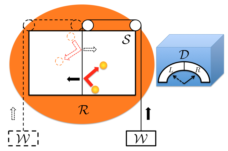
By considering an infinite ensemble of such boxes, the average state of the particle can be interpreted as being an ideal gas occupying volume for which, after feedback, “expands” to volume . If the box is in thermal contact with a single reservoir of temperature , and the gas expands quasistatically, the engine will extract units of work, where is Boltzmann’s constant. This is of course an average quantity of work, taken over the infinite ensemble of boxes. Moreover, the source of the extracted work is the heat drawn from the thermal reservoir. As the (average) state of the system at the start and end of the process is the same – an ideal gas occupying volume – the Szilard engine is in apparent violation of the Kelvin statement of the second law; it is a cyclically operating device, the sole effect of which is to absorb energy in the form of heat from a single thermal reservoir and to produce an equal amount of work [6].
As shown by Penrose and Bennett [7, 8, 9], one may salvage the second law by observing that the demon is itself a physical entity, whose memory is altered by the measuring process. In order to make the engine cyclical the demon’s memory must be returned to its initial configuration, i.e., the demon’s memory must be “reset” or “erased”. If the erasure process is conducted by means of an interaction with the same thermal reservoir, it will require an average work cost no less than the average extracted work, which is dissipated as heat to the reservoir [10, 11, 12]; we may never win in the long run.
In recent years, much attention has been paid to the interplay between quantum theory and thermodynamics [13, 14, 15, 16, 17, 18, 19, 20, 21, 22, 23]. This has included the extension of work extraction through feedback control to the quantum regime, culminating in both theoretical [24, 25, 26, 27, 28, 29] and experimental [30, 31] investigations. Of particular interest to our discussion is the work presented in [32, 33], wherein the authors consider the possibility of a Maxwell demon engine that functions in thermal isolation. Here, the source of work can no longer be identified as heat from a thermal reservoir, but rather as the energetic changes due to projective measurements. Such quantum measurements, however, ultimately result from a physical interaction between the system to be measured, and the measuring apparatus; in the case of a Szilard engine, the measuring apparatus is the demon’s memory. It stands to reason, therefore, that energetic considerations come to bear on the measuring process [34, 35, 36, 37, 38], which will pose limitations on the performance of Szilard engines that, in lieu of a thermal reservoir, draw power from projective measurements.
We recall from the classical Szilard engine that hidden entropy sinks, when the demon’s memory is not explicitly accounted for, allow for a violation of the second law. Similarly, hidden work sources involved in the measuring process can also allow us to “cheat”. Consequently, a constraint of primary importance that must be imposed on the measuring process of a Szilard engine is energy conservation; if the energy of the system is increased by projective measurements, the demon’s energy must decrease in kind. A central result from quantum measurement theory that is relevant to us is the Wigner-Araki-Yanase theorem [39, 40, 41, 42, 43, 44] which, under additive conservation laws, will limit the observables that can be measured. Using this, we shall show that while a Szilard engine can be powered by projective measurements instead of heat from a reservoir, it will have to give up at least one of three features that are present in the classical Szilard engine. The three features of the classical Szilard engine in question are:
Feature 1.
The measurement is repeatable. If the demon measures the box and finds that the particle was on the right (left) hand side, a subsequent measurement would reveal that the particle is on the right (left) hand side with certainty. This allows for the interpretation that, after the measurement has been completed, the system “possesses” the revealed value.
Feature 2.
The weight’s entropy does not change as a result of work extraction. Work is extracted by raising the weight, thus increasing its gravitational potential energy. In general, the height of the weight’s center of mass will be a fluctuating quantity, with an uncertainty . However, does not change as a result of work extraction. In other words, the weight is neither “cooled” nor “heated” as it is elevated.
Feature 3.
The engine works reliably – the work extracted is strictly positive for all measurement outcomes. Whether the particle is on the right or left hand side of the box, the extracted work has the value where . As and are always positive, finite numbers, then for all .
2 Modeling a quantum Szilard engine
A general quantum Szilard engine is constituted of four subsystems: a system ; a demon ; a weight ; and a thermal reservoir . These have the Hilbert space , and respectively the Hamiltonians , , , and . When describing operators that act non-trivially on only one subsystem, we shall omit identities on the other subsystems for simplicity. Furthermore, we shall only consider finite-dimensional Hilbert spaces. This model has in common with [45, 46] and [29, 38] that it includes respectively the weight and the demon’s memory within the quantum description. As with the classical Szilard engine, each cycle of our quantum Szilard engine involves two stages, namely, measurement and feedback. Before can perform measurements in the next cycle, its memory must first be erased. This is achieved by an appropriate interaction with . As the state of can be different at the end of the cycle, then unlike the classical Szilard engine, the quantum Szilard engine is, strictly speaking, not cyclical. However, as will be shown, such non-cyclicality will not result in a violation of the second law.
All Szilard engines must satisfy the following two requirements. Here, we shall state them colloquially, but will offer mathematically precise formulations in the next two subsections.
Requirement 1.
Both the measuring and feedback processes must be energy conserving on the total system.
This is necessary for all work sources to be explicitly accounted for; if either the measuring or feedback process does not conserve the energy of the total system, then it will require work from an outside source.
Requirement 2.
If the demon’s memory is in a state corresponding to a measurement outcome , the feedback process must result in a closed evolution of the compound of system plus weight (and reservoir, if it is present). After feedback, the demon’s memory must remain in the same state.
This is necessary in order to conform with the functioning of the classical Szilard engine described above. There, upon discovering the particle’s location, the demon arranges the weight-and-pulley mechanism accordingly so as to facilitate work extraction. After making its arrangements, the weight, system, and reservoir evolve as a closed, mechanically isolated system, while the demon’s memory is unaltered.
In the subsequent sections, we shall depart from the traditional set-up of the Szilard engine by altering the feedback stage; this will no longer involve , and the source of work will not be identified as heat from the reservoir, but rather the internal energy of the compound . Each cycle of work extraction is depicted schematically in Fig. 2. Our work is similar in spirit to that of [33], except that we model both the weight and demon’s memory as explicit quantum systems, and impose energy conservation on the measuring process.

2.1 Measurement stage
During the measurement stage, the demon performs a measurement on , and by doing so prepares it in a state that is correlated with the measurement outcome. For now, we will restrict ourselves to standard, non-degenerate projective measurements, and shall generalise to degenerate observables in Appendix (C 3.2). If , the observable can be represented as the self-adjoint operator
| (2.1) |
where are the measurement outcomes. Here is a projection on the vector . We wish to model the measurement of as resulting from a physical interaction between and , so that the outcomes are stored in the memory of by the orthogonal set of states . Therefore, we describe the measurement model of , as defined in Eq. (2.1), by the tuple [47, 48, 49, 50, 51]. Here is the initial state of ; is the premeasurement unitary interaction between and , characterised by
| (2.2) |
where can be any set of vectors on , which do not have to be orthogonal; and
| (2.3) |
is an observable on with each outcome corresponding to the same for . Here, is a projection operator of arbitrary rank, such that for all , . If , then .
For an arbitrary initial state of , the total state of after premeasurement is
| (2.4) |
In order for the measuring process to leave a classical record of outcomes, the demon’s memory must be objectified [52]. That is to say, after coupling with by the premeasurement unitary as defined by Eq. (2.2), thus preparing the entangled state as defined in Eq. (2.4), we must prepare the statistical mixture
| (2.5) |
where
| (2.6) |
is the Born rule probability of observing outcome , given a measurement of on , prepared in state . Eq. (2.5) is a proper mixture, or a Gemenge , which can be interpreted as each state being prepared according to a probability distribution , as given by Eq. (2.6). Moreover, can be interpreted as the set of post-measurement states on . We may objectify by performing an unselective Lüders measurement of [50], as defined in Eq. (2.3), on . Alternatively, as shown in [38], can be objectified by unitarily coupling it with an auxiliary system. In the subsequent section we show that imposing Requirement 2 on the feedback process implies that it does not matter whether we objectify the demon before or after the feedback stage.
Definition 1.
Consider a system with Hilbert space and Hamiltonian . The completely positive, trace preserving (CPTP) map is said to conserve energy if
| (2.7) |
for all states on .
Lemma 1.
Proof.
Lemma 2.
Proof.
The post-measurement state of , conditional on outcome , is . The probability of observing outcome in a subsequent measurement of will be , as determined by Eq. (2.6). This equals unity if and only if . Therefore, must be eigenvectors of .
To show that must be eigenvectors of if the measurement is repeatable, we use the WAY theorem. The WAY theorem can be stated thusly: let the premeasurement unitary operator in the measurement model of , i.e., , commute with . If the measurement of is repeatable, or , where is defined in Eq. (2.3), then . We refer to [42] for a proof. If commutes with , then they will share the same eigenvectors. ∎
2.2 Feedback stage
During the feedback stage, the demon brings the system in contact with the weight, , which is initially prepared in state . Conforming with Requirement 2, the demon then evolves the compound system of by the unitary operator , which is chosen conditional on the measurement outcome . We wish to determine the global feedback unitary operator that achieves this.
Lemma 3.
Proof.
Requirement 2 states that if the demon is in a state corresponding to a measurement outcome , the system and weight must undergo a closed evolution. Consequently, must satisfy
| (2.10) |
for all and , where is an eigenstate of the demon observable as defined in Eq. (2.3). This is clearly satisfied if is of the form Eq. (2.9). To prove only if, we note that Eq. (2.10) implies that
| (2.11) |
for all , where is a projection on the subspace of that contains . Therefore, it follows that
| (2.12) |
and so must be of the form Eq. (2.9). ∎
Corollary 1.
Let the feedback unitary satisfy Requirement 2. Then the state of the compound will be identical whether is objectified prior to feedback, or after it.
Proof.
The compound of after premeasurement and objectification is given by Eq. (2.5). After feedback, the state of the compound is
| (2.13) |
If the feedback unitary is of the form Eq. (2.9), then for all , and so we have
| (2.14) |
The second line corresponds to performing feedback after premeasurement, but before objectification has occurred. ∎
Lemma 4.
Proof.
In order for as defined by Eq. (2.9) to conserve the total energy, by Definition 1 we require that
| (2.15) |
for all states on , where . Therefore, must commute with the total Hamiltonian. Because of the additivity of the Hamiltonian, can be written as
| (2.16) |
Given an arbitrary pair of states and , such that , and referring to the right hand and left hand sides of Eq. (2.16) as RHS and LHS, respectively, we see that
| (2.17) |
However, given Eq. (2.16), we must have . This is satisfied if either: (i) for ; or (ii) . Option (i) satisfies the if statement of the Lemma. Option (ii) implies that Eq. (2.16) is satisfied if
| (2.18) |
for all maximal subsets such that, given all , . Here we define .
Eq. (2.18) is satisfied if : (a) and ; or (b) if and . It is easy to verify that (a) is impossible, and so only option (b) is available. This concludes the proof of the only if portion of the Lemma. ∎
For each measurement outcome , as a result of the global feedback unitary operator given in Eq. (2.9), and undergo the complementary CPTP maps
| (2.19) |
where we recall that are the post-measurement states of .
We now wish to define the (average) work that is transferred from into , for each measurement outcome, as a result of feedback. To this end, we use the following definition.
Definition 2.
For each measurement outcome , the average work transferred into the weight is defined as
| (2.20) |
where: is the CPTP map defined by Eq. (2.19);
| (2.21) |
is the non-equilibrium free energy of a system with state , relative to the Hamiltonian and temperature ; and is the von-Neumann entropy of .
This definition has been argued for previously in [53, 54]. Even though the thermal reservoir is not involved during feedback, it is still part of the thermodynamic context of the Szilard engine. As such, work can be extracted from both the system, and the weight, by letting them interact appropriately with the reservoir. Therefore, the quantifier of work transfer must be temperature dependent, in the form of free energy difference, in order to : (i) ensure consistency with the “internal” description of work extraction from , wherein the weight is not included in the quantum description; and (ii) avoid violation of the second law. For a detailed argument we refer the reader to Appendix (A). We note that an alternative definition for work transfer to the weight is the increase in the internal energy of . While this formulation will be consistent with the second law only if the feedback unitary induces unital dynamics on the system [55], Definition 2 does not suffer from such limitations. Moreover, Definition 2 reduces to the increase in internal energy when Feature 2 is satisfied.
Now that we have defined work extraction, we may analyse this with respect to Feature 2.
Definition 3.
The Szilard engine satisfies Feature 2 if for all ,
| (2.22) |
Lemma 5.
3 The impossibility theorem

We are now ready to prove a main result of this paper. The impossibility theorem is illustrated by Penrose’s impossible triangle in Fig. 3.
Theorem 1.
Proof.
Let the engine satisfy Feature 1 and Feature 2. By Lemma 2 the post-measurement states are the eigenvectors of and, hence, . Consequently, for some outcome , . By Lemma 5, for this outcome we have , and Feature 3 cannot be satisfied.
Theorem 1, simply stated, says that if the system is measured with respect to a non-degenerate observable, in a repeatable and energy conserving fashion, it must be projected onto the eigenstates of . Consequently, if we do not allow the weight’s entropy to decrease, then for the outcome that projects the system onto the groundstate of , zero work can be extracted.
In Appendix (B), we illustrate the incompatibility between the three features by looking at a concrete model where both and are qubits, while is a harmonic oscillator. In Appendix (C) we show that Theorem 1 can be circumvented if: (i) the thermal reservoir is involved during the feedback stage so that, just as in the classical Szilard engine, the source of work will be heat drawn from the reservoir; or (ii) the observable measured on is degenerate and is measured “inefficiently”.
4 Net work extraction per cycle
Fig. 2 depicts a single cycle of the Szilard engine under consideration. In Appendix (D) we evaluate the net work extraction per cycle, wherein we do not distinguish between measurement outcomes. Labeling the “coarse-grained” work transferred to the weight as , and the work cost of erasure as , the net coarse-grained work is shown to obey the inequality
| (4.1) |
where and are the average states of and at the end of the cycle, respectively, obtained by sampling the states and by the probability distribution as defined by Eq. (2.6). We note that Eq. (4.1) holds irrespective of whether the Szilard engine satisfies any of Feature 1, Feature 2, or Feature 3. Moreover, we note that the coarse-grained work is generally smaller than the average work, i.e., , where is defined in Eq. (2.20). While the coarse-grained work extraction obeys the second law, the average work will not; if is thermal, then whereas can be positive.
To be sure, the second law is a statistical statement, held true precisely when we do not have access to the individual measurement outcomes. Let us recall the definition for work transferred into the weight when it transforms as , given by Definition 2 and articulated in Appendix (A). This was given operational meaning as being the maximum value of work that can be extracted from the weight, by an isothermal process involving the reservoir of temperature . However, if we were to forget the measurement outcomes, then we could not use such information to tailor our process of extracting work from the weight. Indeed, this protocol must be designed with only the average state of the weight in mind. The maximum value of work extractable from the weight, given an isothermal process , is precisely .
5 Discussion
We give a general mathematical description of a quantum Szilard engine that operates in two stages, namely, projective measurement and feedback. In our model, in contradistinction to the classical Szilard engine, the feedback stage does not involve the thermal reservoir. Here, the source of work is the energetic changes due to (non-degenerate) projective measurements. In order to avoid cheating by the inclusion of hidden work sources, we impose energy conservation on the measuring process. As a result of the Wigner-Araki-Yanase theorem, the observables that the demon can measure will be limited to those that commute with the system’s Hamiltonian.
We showed that while the Szilard engine, in lieu of a thermal reservoir, can be powered by (non-degenerate) projective measurements, it cannot simultaneously satisfy three features of the classical Szilard engine model; the conjunction of any two will preclude the possibility of the third. These features are: (i) the measurement performed by the demon is repeatable, meaning that conditional on obtaining outcome , a subsequent measurement of the same observable would yield with certainty; (ii) the weight’s entropy does not change as a result of feedback; and (iii) work extraction is reliable, i.e., is strictly positive for all measurement outcomes. This observation is a first step towards developing “second-law-like” relations in the context of measurement-assisted feedback control beyond thermality. While the second law results from entropic considerations, these “second-law-like” relations would result from energy conservation of unitary interactions that implement measurements.
The Szilard engine here discussed is, strictly speaking, not cyclical; at the end of a cycle of work extraction, the state of the system, , will not be the same as its initial state, . For the engine to be made cyclical, therefore, we must have at our disposal an infinite supply of systems with state such that, at the end of each cycle, the system’s state is swapped with one of these. One example of such “free resources” is if is thermal. Here, we may interpret the closure of the cycle to result from the system being brought to thermal equilibrium with the reservoir.
The strict non-cyclicality of the engine notwithstanding, the statistical second law will not be violated. This is because, when taking the erasure cost of the demon into consideration, the total net work extracted from the system will be bounded by the decrease in its free energy – a quantity that will not be positive if the system is initially at thermal equilibrium. However, this requires a careful consideration of how one should evaluate work when choosing to “forget” the measurement outcomes – precisely the domain where the second law is applicable. As with unselective measurements, the work transferred to the weight when the indvidual measurement outcomes are not distinguished from one another must be defined by how the weight’s state changes on average. Indeed, the extractable work from the weight, when the measurement outcomes are forgotten, is smaller than the average value of work, when the measurement outcomes are taken into consideration.
Acknowledgements.
The authors would like to thank L. D. Loveridge, K. Abdelkhalek, D. Reeb, K. Hovhannisyan, and H. Miller for the useful discussions that helped in developing the ideas presented in this paper. J. A. acknowledges support from EPSRC, grant EP/M009165/1, and the Royal Society. This research was supported by the COST network MP1209 “Thermodynamics in the quantum regime”.References
- [1] T. Sagawa and M. Ueda, Phys. Rev. E 85, 021104 (2012).
- [2] N. Shiraishi, S. Ito, K. Kawaguchi, and T. Sagawa, New J. Phys. 17, 045012 (2015).
- [3] J. C. Maxwell, Theory of Heat (Longmans, 1871).
- [4] K. Maruyama, F. Nori, and V. Vedral, Rev. Mod. Phys. 81, 1 (2009).
- [5] L. Szilard, Zeitschrift fuer Physik 53, 840 (1929).
- [6] R. Balian, From Microphysics to Macrophysics: volume 1 (Springer, 2007).
- [7] O. Penrose, Foundations of Statistical Mechanics: A Deductive Treatment (Pergamon, 1970).
- [8] C. H. Bennett, Int. J. Theor. Phys. 21, 905 (1982).
- [9] C. H. Bennett, Studies in History and Philosophy of Modern Physics 34, 501 (2003).
- [10] R. Landauer, IBM J. Res. Dev. 5, 183 (1961).
- [11] R. Landauer, Physics Letters A 217, 188 (1996).
- [12] D. Reeb and M. M. Wolf, New J. Phys. 16, 103011 (2014).
- [13] S. Vinjanampathy and J. Anders, Contemp. Phys. 57, 545 (2016).
- [14] J. Goold, M. Huber, A. Riera, L. del Rio, and P. Skrzypczyk, Journal of Physics A: Mathematical and Theoretical 49, 143001 (2016).
- [15] J. Millen and A. Xuereb, New J. Phys. 18, 011002 (2016).
- [16] M. Horodecki and J. Oppenheim, Nature Communications 4, 2059 (2013).
- [17] P. Kammerlander and J. Anders, Scientific Reports 6, 22174 (2015).
- [18] M. Lostaglio, D. Jennings, and T. Rudolph, Nature Communications 6, 6383 (2015).
- [19] M. Perarnau-Llobet, K. V. Hovhannisyan, M. Huber, P. Skrzypczyk, N. Brunner, and A. Acín, Phys. Rev. X 5, 041011 (2015).
- [20] C. Gogolin and J. Eisert, Reports on Progress in Physics 79, 056001 (2016).
- [21] Y. Guryanova, S. Popescu, A. J. Short, R. Silva, and P. Skrzypczyk, Nature Communications 7, 12049 (2016).
- [22] N. Yunger Halpern, P. Faist, J. Oppenheim, and A. Winter, Nature Communications 7, 12051 (2016).
- [23] Á. M. Alhambra, L. Masanes, J. Oppenheim, and C. Perry, Phys. Rev. X 6, 041017 (2016).
- [24] W. H. Zurek, “Maxwell’s demon, szilard’s engine and quantum measurements,” in Frontiers of Nonequilibrium Statistical Physics, edited by G. T. Moore and M. O. Scully (Springer US, Boston, MA, 1986) pp. 151–161.
- [25] M. Plesch, O. Dahlsten, J. Goold, and V. Vedral, Scientific Reports 4, 6995 (2014).
- [26] S. W. Kim, T. Sagawa, S. De Liberato, and M. Ueda, Phys. Rev. Lett. 106, 070401 (2011).
- [27] T. Sagawa and M. Ueda, Phys. Rev. Lett. 100, 080403 (2008).
- [28] K. Jacobs, Phys. Rev. A 80, 012322 (2009).
- [29] J. J. Park, K.-H. Kim, T. Sagawa, and S. W. Kim, Phys. Rev. Lett. 111, 230402 (2013).
- [30] P. A. Camati, J. P. S. Peterson, T. B. Batalhão, K. Micadei, A. M. Souza, R. S. Sarthour, I. S. Oliveira, and R. M. Serra, Phys. Rev. Lett. 117, 240502 (2016).
- [31] N. Cottet, S. Jezouin, L. Bretheau, P. Campagne-Ibarcq, Q. Ficheux, J. Anders, A. Auffèves, R. Azouit, P. Rouchon, and B. Huard, ArXiv: 1702.05161 .
- [32] C. Elouard, D. Herrera-Martí, M. Clusel, and A. Auffèves, npj Quantum Information 3 (2017).
- [33] C. Elouard, D. Herrera-Martí, B. Huard, and A. Auffèves, Phys. Rev. Lett. 118, 260603 (2017).
- [34] T. Sagawa and M. Ueda, Phys. Rev. Lett. 102, 250602 (2009).
- [35] K. Jacobs, Phys. Rev. E 86, 040106 (2012).
- [36] M. Navascués and S. Popescu, Phys. Rev. Lett. 112, 140502 (2014).
- [37] T. Miyadera, Foundations of Physics 46, 1522 (2016).
- [38] K. Abdelkhalek, Y. Nakata, and D. Reeb, ArXiv: 1609.06981 .
- [39] E. Wigner, Z. Phys. 133, 101 (1952).
- [40] H. Araki and M. M. Yanase, Phys. Rev. 120, 622 (1960).
- [41] T. Miyadera and H. Imai, Phys. Rev. A 74, 024101 (2006).
- [42] L. Loveridge and P. Busch, The European Physical Journal D 62, 297 (2011).
- [43] P. Busch and L. Loveridge, Phys. Rev. Lett. 106, 110406 (2011).
- [44] M. Ahmadi, D. Jennings, and T. Rudolph, New J. Phys. 15, 013057 (2013).
- [45] P. Skrzypczyk, A. J. Short, and S. Popescu, Nature Communications 5 (2014).
- [46] J. Åberg, Phys. Rev. Lett. 113, 150402 (2014).
- [47] J. von Neumann, Mathematical Foundations of Quantum Mechanics (Princeton University Press, 1996).
- [48] P. Busch, M. Grabowski, and P. J. Lahti, Operational Quantum Physics (Springer, 1995).
- [49] P. Busch, P. J. Lahti, and P. Mittelstaedt, The Quantum Theory of Measurement (Springer, 1996).
- [50] P. Busch, P. J. Lahti, J. P. Pellonpää, and K. Ylinen, Quantum Measurement (Springer, 2016).
- [51] T. Heinosaari and M. Ziman, The Mathematical Language of Quantum Theory (Cambridge University Press, 2011).
- [52] P. Mittelstaedt, The Interpretation of Quantum Mechanics and the Measurement Process (Cambridge University Press, 2004).
- [53] J. Gemmer and J. Anders, New J. Phys. 17, 085006 (2015).
- [54] R. Gallego, J. Eisert, and H. Wilming, New J. Phys. 18, 103017 (2016).
- [55] Y. Morikuni, H. Tajima, and N. Hatano, Physi. Rev. E 95, 032147 (2017).
- [56] J. Anders and V. Giovannetti, New J. Phys. 15, 033022 (2013).
- [57] P. Alberti and A. Uhlmann, Stochasticity and Partial Order: Doubly Stochastic Maps and Unitary Mixing (Springer, 1982).
- [58] M. Nakahara, R. Rahimi, and A. Saitoh, Decoherence Suppression in Quantum Systems (World Scientific, 2008).
- [59] D. Petz, Quantum Information Theory and Quantum Statistics (Springer, 2008).
Appendix A Definition of work transferred into the weight
Here we wish to justify defining the work transferred into the weight, as a result of feedback, by Definition 2. To this end, let us first recall a known result from standard non-equilibrium quantum thermodynamics. In the internal description of work extraction, in contradistinction to the external description, the weight is not included in the quantum formalism. Here, the work extracted from a system undergoing a (non-energy conserving) unitary evolution is defined as the decrease in its internal energy. Consequently, if a system undergoes a transformation , where is a global unitary operator and is the thermal state of the thermal reservoir , with the inverse temperature, the work extracted obeys the inequality
| (A.1) |
with the equality obtained when the interaction between system and thermal reservoir is “quasi-static” [56].
Therefore, Definition 2 can be justified with the following argument. When the weight interacts with the system, thereby transforming as , where is given by Eq. (2.19), work is transferred to it. We may then perform the reverse transformation on the weight, i.e., , by an appropriate unitary interaction with the thermal reservoir, so as to extract this work. The work extracted here will be in the internal description, as there is no second weight into which the work is being transferred. By Eq. (A.1), the work we may extract obeys the inequality
| (A.2) |
Clearly, the work transferred into the weight must be at least as great as the work that can be extracted from the weight, i.e.,
| (A.3) |
A natural assumption to make is that, since the process of transferring work into the weight is independent of the process by which work is extracted from the weight, the right hand side of the above equation should be replaced by the upper bound of Eq. (A.2). If we also take the view that transferring more work into the weight than can possibly be extracted from it is physically meaningless, we arrive at Definition 2.
We also note that Definition 2 is consistent with the internal description of work from the system , and that it satisfies the second law.
Lemma 6.
Let the system and weight be initially prepared in the states and , respectively. Let the two systems evolve by a unitary operator that conserves the total Hamiltonian , and induces the complementary CPTP maps on and on . Then the work transferred into the weight, , as defined by Definition 2, will never exceed the maximum work that can be directly extracted from the system by the process , in the internal description, and using a single thermal reservoir at temperature . If is thermal, then cannot be positive.
Proof.
By Definition 2, energy conservation of , and the subadditivity of the von-Neumann entropy, we have
| (A.4) |
By Eq. (A.1), we see that is never greater than the upper bound of . Moreover, if the system is initially in the thermal state , we have
| (A.5) |
where is the entropy of relative to , which is a non-negative number and vanishes if and only if . Therefore, . ∎
Appendix B An example with qubits
As an illustrative example, consider the simple case where and are both qubits, with the Hamiltonians
| (B.1) |
Furthermore, let the initial state of the system be
| (B.2) |
while that of is . We wish to measure a two-valued observable , with outcomes , with the measurement model . In order to satisfy Requirement 1 for the measuring process, as shown by Lemma 1 and Lemma 2, and must commute with and , respectively. Therefore, we choose
| (B.3) |
and
| (B.4) |
Given our choice of and , the premeasurement unitary operator is chosen as
| (B.5) |
Finally, in order for the engine to satisfy Requirement 1 and Requirement 2 for the feedback process, we choose the global feedback unitary operator
| (B.6) |
Following [46], we will use a harmonic oscillator of frequency as the weight, with the Hamiltonian
| (B.7) |
Consequently, the conditional work extraction unitaries on , namely, , can be constructed as
| (B.8) |
where and , with . Here, is a unitary operator on , such that . Therefore, when the system undergoes a transition , the weight eigenstates are shifted up by one quantum, and vice versa.
It can be easily verified that , even when are not eigenstates of the system Hamiltonian. If the weight is initialised in a pure state , where is an equal superposition of Hamiltonian eigenstates,
| (B.9) |
then it can function as a work storage device. This is a result of the energy-translational invariance of ; adding or removing one quantum is identical to a coordinate transformation and , respectively. Moreover, if are the eigenvectors of , then irrespective of the resulting dynamics on both and will be unitary. As such, Feature 2 will be satisfied in this case. This is not so when are superpositions of eigenvectors. For example, in the case of , we have
| (B.10) |
with
| (B.11) |
In the limit as tends to infinity, the increase in the weight’s entropy can be made arbitrarily small, thus approximately satisfying Feature 2.
We now look at two possible implementations of measurement-assisted work extraction, labeled I and II. In I, the observable is measured repeatably, thus satisfying Feature 1, while in II this is not the case. As the weight is initially pure, its entropy can never decrease. Therefore, Feature 3 is satisfied in II, but not in I.
2.1 Example I: repeatable measurement
Let , thus satisfying Feature 1. Consequently, the state of after premeasurement is
| (B.12) |
Transforming this state with the weight by the global unitary prepares
| (B.13) |
Comparing Eq. (B.12) with Eq. (B.13), we see that, as a result of feedback, the system undergoes the transition when the demon is in the state , resulting in a work extraction of . When the demon is in the state , on the other hand, the system was already in the groundstate and is left the same, resulting in zero work extraction. Therefore, Feature 3 is not satisfied.
2.2 Example II: non-repeatable measurement
Let . Hence, Feature 1 is not satisfied. Consequently, the state of after premeasurement is
| (B.14) |
Transforming this state with the weight by the global unitary prepares, in the ideal limit of ,
| (B.15) |
Comparing Eq. (B.14) with Eq. (B.15) we see that, as a result of feedback, the system undergoes the transition when the demon is in the states , resulting in a work extraction of for both measurement outcomes. Therefore, Feature 3 is satisfied.
Appendix C Satisfying all three features with either a thermal reservoir, or degenerate observables
There are at least two ways in which Theorem 1 can be circumvented: (i) letting the reservoir be involved during the feedback stage; and (ii) measure with a degenerate observable.
3.1 Szilard engine with heat from a thermal reservoir
As a simple example, let be a -dimensional system, and let be a system initially prepared in the thermal state
| (C.1) |
where is the inverse temperature. By Lemma 2, the non-degenerate observable can only be measured repeatably if it commutes with the system Hamiltonian . As such, in order to satisfy Feature 1 the post-measurement states must be eigenstates of . Including the reservoir in the feedback stage means that the in the feedback unitary operator defined in Eq. (2.9) are unitary operators on the compound such that . The CPTP maps defined in Eq. (2.19) will therefore be modified as
| (C.2) |
The subadditivity of the von-Neumann entropy and its invariance under unitary evolution implies that
| (C.3) |
Recalling that when Feature 2 is satisfied, , then by Definition 2 and Eq. (C.3), the work that can be extracted for each measurement outcome, when both Feature 1 and Feature 2 are satisfied, is bounded by
The final inequality can be saturated when the relative entropy term, , which is a non-negative number, is made vanishingly small. As shown in [12], this can be done if the dimension of is chosen to be sufficiently large, and its Hamiltonian spectrum is carefully chosen. As can be positive even when the weight’s entropy is not allowed to change, we can always have positive work extraction. This is true even if the post-measurement state is the groundstate of . Moreover, if is fully degenerate, and , then the maximum value of will be for all . If , this coincides with the work extracted from the classical Szilard engine when the volumes of the left and right side of the partition are identical.
3.2 Degenerate observables
Recall that Theorem 1 states that, when Feature 2 is satisfied, then the extracted work will not be positive for the outcome where the post-measurement state coincides with the groundstate of the system Hamiltonian. Here we show that, if the observable is both degenerate and is measured “inefficiently”, then the post-measurement states can always be chosen so as to have more energy than the groundstate of , thus allowing for the circumvention of Theorem 1.
For a system with Hilbert space such that , let be a degenerate observable
| (C.4) |
such that , and is a complete and orthogonal set of projection operators on . We label the orthonormal eigenstates of as , where is a degeneracy label, such that for all and . The measurement model for this observable, , will be repeatable if for all , the post-measurement states lie in the support of . Moreover, by the WAY theorem, if is to be repeatable, given that conserves the total Hamiltonian, then must commute with for all . Consider the projector whose support contains the groundstate(s) of . It follows that for a repeatable measurement, is the only outcome whose post-measurement state will have support on the groundstate(s) of . Therefore, in order to circumvent Theorem 1 we need to show that, for all , the post-measurement state given outcome has more energy than the minimum eigenvalue of .
We will now look at two repeatable, and energy conserving measurement models for the degenerate observable . The first model is a generalisation of a Lüders measurement [52, 51]. Here, for some state , the post-measurement state of outcome is the groundstate of . Consequently, this measurement model will not circumvent Theorem 1. In the second model, we may always ensure that the post-measurement state for outcome will have more energy than the groundstate, thus circumventing Theorem 1. We show that this is equivalent to coarse-graining the measurement outcomes of a non-degenerate observable, in such a way so as to allow for a repeatable measurement that is also “inefficient”.
3.2.1 Strong value-correlation measurements
These measurements, just as the standard measurements for non-degenerate observables, have the property that, for any pure state , the post-measurement state for outcome will also be pure. Here, the premeasurement unitary operator is
| (C.5) |
where is an orthonormal basis that spans . The instrument implemented by this measurement model will be
| (C.6) |
where is a unitary operator acting on the support of . This instrument has only one Kraus operator, , and it is said to result in an “efficient” measurement. If , whereby , we have a Lüders measurement.
If the system is initially in the pure state
| (C.7) |
the post-measurement state for outcome will be
| (C.8) |
Therefore, for some state , the post-measurement state will be equal to the groundstate of the Hamiltonian. As such, Theorem 1 will not be circumvented.
3.2.2 Coarse-grained standard measurements
Let us denote the degenerate eigenstates of as the orthonormal set of vectors such that for all and . The premeasurement unitary operator can then be defined as
| (C.9) |
Comparing with Eq. (2.2), we may see this as a coarse-grained measurement of a standard, non-degenerate observable. Now, the vectors in no longer have to be orthonormal. But, they must still be eigenstates of with eigenvalue for the measurement to be repeatable. The instrument implemented by this measurement model will be
| (C.10) |
where are unitary operators acting on the support of . In contrast to the generalised Lüders measurement discussed previously, this instrument has more than one Kraus operator, and leads to an “inefficient” measurement.
If the system is initially in the pure state
| (C.11) |
the post-measurement state for outcome will be
| (C.12) |
Due to the orthogonality of the vectors in Eq. (C.9), for each and , the vectors can be any superpositions of Hamiltonian eigenstates that live in the support of . So we may simply choose these as the highest energy state within that subspace. Consequently, Theorem 1 will be circumvented.
Appendix D Net work extraction per cycle of a quantum Szilard engine without heat from a thermal reservoir
Each cycle of work extraction involves the following steps: (i) is given in state ; (ii) and undergo a joint unitary evolution by ; (iii) work is extracted from by a feedback unitary operator on ; (iv) is reset to its initial state by coupling to a thermal reservoir. Fig. 2 shows this schematically.
The initial state of the compound is
| (D.1) |
where is the Gibbs state of the reservoir at inverse temperature . After premeasurement, objectification, and feedback the state will be
| (D.2) |
where is defined in Eq. (2.5). The marginal states of satisfy the relations
| (D.3) |
where is the Born rule probability defined in Eq. (2.6), while and are the CPTP maps induced by feedback, as defined in Eq. (2.19).
Using Definition 2, we may view the work transferred into the weight, when the different measurement outcomes are not distinguished from one another, to be
| (D.4) |
Here we have used the fact that feedback and measurement are energy conserving on the total system. We call the “coarse-grained” work, which is different to the average work, obtained by averaging over all measurement outcomes , which is
| (D.5) |
The inequality here is due to the concavity of the von-Neumann entropy.
Before the cycle can begin anew, the demon must be reset to the original pure state . This is achieved within the Landauer framework, by coupling with by the “erasure” unitary operator . If the reservoir is infinitely large, then can be chosen so that
| (D.6) |
To be sure, is generally not energy conserving, and thus needs a hidden work source. Notwithstanding, this is not a problem, because erasure always consumes work. Therefore, this hidden work source does not contribute to work extraction within a cycle. Defining the reduced state of the reservoir after its interaction with as , the consequent increase in energy of the reservoir, defined as heat, obeys Landauer’s inequality
| (D.7) |
As shown in [12], this bound can be achieved if the reservoir is infinitely large, and its Hamiltonian has a specific spectrum. Furthermore, we note that premeasurement, objectification, and feedback results in a unital CPTP map, which does not decrease the von-Neumann entropy [57, 58]. This, together with the subadditivity of the von-Neumann entropy [59], implies that
| (D.8) |
Consequently, by combining Eq. (D.7) and Eq. (D.8), and also taking into account the energy change of the demon due to erasure, the work cost of erasure is shown to obey the inequality
| (D.9) |
Defining the net coarse-grained work extraction as , by combining Eq. (D.4) and Eq. (D.9) we arrive at the inequality
| (D.10) |
The net average work extraction , on the other hand, obeys the modified inequality
| (D.11) |
Therefore, we see that while the coarse-grained work definition of Eq. (D.4) will satisfy the second law, the average work extraction defined in Eq. (D.5) will not; if is initially thermal, the net coarse-grained work extraction given by Eq. (D.10) will never be positive, whereas the net average work extraction given by Eq. (D.11) could be.