On the features of Matese-Whitman mass function
Abstract
In the present paper we exhaustively examine the physical status of the socalled Matese-Whitman mass function [J.J. Matese and P.G. Whitman, Phys. Rev. D, 22, 1270 (1980)]. As a first step, we construct the relevant Einstein field equations with an anisotropic matter distribution under the approach of Conformal killing Vector. In the intermideate step we find a set of exact solutions by using the Matese-Whitman mass function. Eventually we conduct several physical tests to explore features of the applied mass function in connection to the specific compact stars. It can be observed that all the features of the model based on the Matese-Whitman mass function are of physical interests.
dibyendu_shee@yahoo.com00footnotetext: Department of Physics, Indian Institute of Engineering Science and Technology, Shibpur, Howrah 711103, West Bengal, India
d.deb32@gmail.com00footnotetext: Department of Physics, Indian Institute of Engineering Science and Technology, Shibpur, Howrah 711103, West Bengal, India
shnkghosh122@gmail.com00footnotetext: Department of Physics, Indian Institute of Engineering Science and Technology, Shibpur, Howrah 711103, West Bengal, India
bkguhaphys@gmail.com00footnotetext: Department of Physics, Government College of Engineering and Ceramic Technology, Kolkata 700010, West Bengal, India
saibal@associates.iucaa.in
Keywords general relativity, conformal Killing vector, Matese-Whitman mass function, anisotropic compact stars
I Introduction
A particular type of mass function, known in the literature as the Matese-Whitman mass function [37], that gives a monotonic decreasing matter density can be provided by
| (1) |
where and are two positive constants. It is observed that this mass function has earlier been used by [34] to model an anisotropic fluid star, Lobo [29] to develop a model of dark energy star, Sharma and Maharaj [48] to model a class of relativistic stars with a linear equation of state, and Maharaj and Thirukkanesh [36] to strange stars with quark matter. Further and specific litarure survey on the Matese-Whitman mass function shows that there are some other works done by several authors [45, 2, 9] which are of particular interest.
The compact anisotropic relativistic astrophysical objects are always the field of immense interest to the active astrophysicists. The compact objects are formed at the end point of the stellar evolution and its exact nature is still playing ‘hide and seek’ with the researchers. It is knwon that a neutron star-like compact star is the final stage of a gravitationally collapsed star which, after exhausting all its thermo-nuclear fuel, gets stabilized by degenerate pressure.
The first exact solution of Einstein field equations for the interior of a compact object was obtained by Schwarzschild in 1916, after that several relativists obtained other exact solutions. Delgaty and Lake [11] analysed that out of 127 published solutions only 16 solutions satisfy all the physical conditions. Mak and Harko [33] were obtained an exact solution of Einstein field equations, describing spherically symmetric and static anisotropic stellar configuration, by assuming a particular form of anisotropic factor. Ruderman [47] has shown that the nuclear matter may have anisotropic features at very high density ranges ( gm/c.c.). At this range the nuclear interactions must be treated relativistically. As a result of the anisotropy, pressure inside the fluid sphere can be decomposed into two parts namely radial pressure and tangential pressure , where is in the perpendicular direction to .
It has been argued that anisotropy may occurs in various reasons, e.g., the existence of external field, in presence of type superfluid, rotation, phase transition, magnetic field, mixture of two fluids, existence of solid core etc. Including the effect of local anisotropy, Bowers [4] showed that anisotropy may have non-negligible effects on the parameters like maximum equilibrium mass and surface redshift. Herrera and Santos [22] have studied local anisotropy in self gravitating systems. For modeling the compact astrophysical objects physically and more realistically (with or without cosmological constant), several astrophysicists have chosen anisotropic matter distribution which are in the literature [33, 34, 50, 25, 23, 38, 43, 26]. According to Usov [50] the reason for consideration of anisotropy within the compact star could be the presence of strong electric field. Egeland [12] studied mass and radii of neutron stars by incorporating the existence of cosmological constant proportionality which depends on the density of vacuum and by using the Fermi equation of state together with the Tolman-Oppenheimer-Volkov (TOV) equation.
CKV is a elegant technique by which one can search for the inheritance symmetry which provides a natural relationship between geometry and matter through the Einstein field equation. Several studies have been done on charged or neutral fluid spheres with a spacetime geometry that admits a conformal symmetry, in the static as well as non-static cases. Long ago Herrera and his co-workers [18, 19, 20, 21] have extensively studied the interior solutions admitting conformal motions. However, there are lots of recent works on the conformal symmetry available in the following literature [44, 45, 15, 39, 1, 13, 27, 41, 8, 49].
Now under the above historical background our motivation and plan of investigation are based on the following steps: in section 2 we have discussed the Einstein field equations under the non-static conformal symmetry and their solutions in section 3 for anisotropic matter distribution. In section 4 by applying the boundary conditions we have found expressions for the constants and the metric potentials. Several physical features have been studied in section 5. Remarks on our model are made in section 6.
II The Einstein field equations under non-static conformal symmetry
The highly nonlinear partial differential equations of Einstein’s gravity can easily be reduced to ordinary differential equations by using the above mentioned technique of CKV.
The interior of a star under conformal motion through non-static Conformal Killing Vector can be represented as in ref. [35, 7, 30, 42]
| (2) |
where represents the Lie derivative operator. It gives the information of the interior gravitational field of a stellar configuration with respect to the vector field and the conformal factor .
Let us consider that our static spherically symmetric spacetime admits an one parameter group of conformal motion. A static, spherically symmetric spacetime can be described by the line element in the standard form as,
| (3) |
Were and are the metric potentials and function of the radial coordinate r only. Here we have considered in geometrized units.
The proposed charged fluid space-time is mapped conformally onto itself along the direction . Here following Herrera and his coworkers [18, 19, 20, 21] we assume as non-static but to be static as follows:
| (4) |
| (5) |
The above set of Eqs. (1)-(4) give the following expressions for , , and from ref. [35, 7, 16, 30, 42, 23]
| (6) |
| (7) |
| (8) |
| (9) |
where , , and are arbitrary constants. According to Maartens and Maharaj [35] one can set , and so that by rescaling we can get
| (10) |
| (11) |
| (12) |
| (13) |
Without loss of any generality one can choose , and . Hence rescaling of and has been done in the following manner, and which leaves Eq. (2) invariant.
Now, we shall consider the most general energy momentum tensor compatible with spherically symmetry in the following form as
| (14) |
with and . Here is the fluid -velocity vector and is the space like vector which is orthogonal to . Also is the matter density, and are respectively the radial and transverse pressure of the anisotropic fluid distribution. Here is in the orthogonal direction to . Actually the anisotropic fluid allows the pressure to differ among spatial direction. is known as anisotropic factor of the spherical system [28, 3].
| (16) |
| (17) |
Imposing the conformal motion, one can write the stress energy components in terms of the conformal function as follows
| (18) |
| (19) |
| (20) |
III Solutions of the field equations
Now our task is to find out solutions for the above set of the modified Einstein equations in terms of the conformal motion. From the mass function (1), the matter density can be obtained as
| (21) |


.
The Fig. 1 shows that is positive inside the star. It decreases with the increase of the radius of the star. We also found from the graph that which implies that density have maximum value at the centre and it decreases monotonically towards the surface.
| (24) |


The variation of radial pressure is shown in Fig. 2, which suffers from a serious problem of singularity. The graph also shows that which implies radial pressure also decreases monotonically the radius of the star.


The graphical representation of the tangential pressure with the radius of the star in Fig. 3 features that decreases maintaining the same pattern as and it also suffers from the singularity problem. implies that it also monotonically decreasing function of .
The simplest form of the barotropic equation of state (EOS) is given by , where are the EOS parameters along the radial and transverse directions. Actually this EOS is used for a spatially homogeneous cosmic fluid though it can be extended to inhomogeneous spherically symmetric spacetime also. The complicated different forms of with its possible space and time dependence are available in the literature [51, 6, 40].
Therefore, the EOS parameter can be written in the following form as
| (25) |


| (26) |
Fig. 4 shows the variation of radial and tangential EOS parameter with respect to the radial distance. From this plot it is clear that EOS does not satisfy the condition . So the underlying matter distribution is exotic in nature.
IV Boundary Condition
Now to derive values of the constants we are matching out interior spacetime with the exterior Schwarzschild metric given as
| (27) |
where and are the effective mass and radius of the stellar system.
Now for a physical stellar the radial pressure should vanish at the surface, i.e., at one have . Imposing this condition we get
| (28) |
Now following the boundary condition for maximized anisotropy at the surface of a compact star [10] we have
| (29) |
Again continuity of the metric potential at the surface, , one can obtain
| (30) |
Hence from Eqs. (29) and (30) we have several values of and we are taking only that value of for which we are getting physically acceptable solution given as
| (31) |

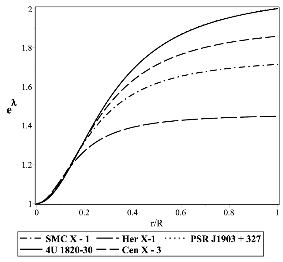
The metric potential can in a straight forward way be derived using Eqs. (12), (21) and (22) as
| (32) |
In a similar way, the metric potential can after some manipulation be derived using Eqs. (13), (32) and (27) as
| (33) |
where
, and .
Features of variation of the metric potentials are shown in Fig. 5.
V Physical features of the model
V.1 Anisotropic behaviour
The measure of anisotropy in pressure can be obtained as
| (34) |
It can be seen that the ‘anisotropy’ will be directed outward when i.e. , and inward when i.e. . Fig. 6 shows the variation of anisotropy with the radius of the star. From the figure it is clear that in general , i.e., though there is a change over at km. This result implies that anisotropic force is repulsive in nature and according to [14] it helps to construct more compact object. It is also to be noted that the anisotropic force dose not vanishes at the centre as expected to develop the model of a star.

V.2 Energy condition
For an anisotropic fluid sphere the energy conditions namely Weak Energy Condition (WEC), Null energy Condition (NEC), Strong Energy Condition (SEC) and Dominant Energy Condition (DEC) are satisfied if and only if the following inequalities hold simultaneously by every points inside the fluid sphere.
| (35) |
| (36) |
| (37) |
| (38) |
We shall prove the inequalities with the help of graphical representation.


From Fig. 7 it is very clear that NEC, WEC, SEC are satisfied by our model.
V.3 TOV equation
To search equilibrium situation of this anisotropic star under different forces, the generalised Tolman-Oppenheimer-Volkoff (TOV) equation can written as
| (39) |
where is the effective gravitational mass inside a sphere of radius which can be derived from the Tolman-Whittaker formula as
| (40) |
Substituting Eq. (33) in Eq. (32) we get the following form of the TOV equation
| (41) |
The Eq. (34) can be rewritten as
| (42) |
where
| (43) |
| (44) |
| (45) |


Here , and are gravitational, hydrostatics, and anisotropic forces respectively. In Fig. 8 profile of the interaction between these three forces are shown in an elegent way. The figure indicates that the combined effects of the gravitational and anisotropic forces is balanced by the hydrostatic force which provides equilibrium configuration of the stellar structure.
V.4 Herrera’s condition for stability analysis
According to causality condition the velocity of sound should follow the condition for a physically realistic model as was proposed by Herrera [17] known as a technique for stability check of local anisotropic matter distribution. This technique dictates that the region for which radial speed of sound is greater than the transverse speed of sound is a potentially stable region. For our anisotropic model, radial and transverse velocity of sound are defined by
| (46) |
| (47) |
where , , , and .


From the Fig. 9 it is very clear that for our model the radial and tangential speed of sound, and also their difference consistent with the Herrera cracking concept but they do not satisfies causality condition. So in the aspect of causality condition we are not getting a stable stellar configuration. This is also true for the adiabatic index and as can be observed from Fig. 10.
V.5 Compactification factor and redshift
The mass of the compact star can be calculated from the density profile
| (48) |

Now the mass function is regular at the origin as . The profile of the mass function shows (see Fig. 11) that mass function is monotonically increasing function of radius.
Since for a compact star, the maximum allowable ratio of the mass to the radius cannot be arbitrarily large so by Buchdahl [5] the ratio of twice the maximum allowable mass to the radius is less than , i.e. where is called the compactification factor which classifies the stellar objects in different categories as shown by Jotania and Tikekar [24]. It is to note that Mak et al. [31] derived a more simplified expression for the same ratio. In the present study we observe that all the stars satisfy the Buchdahl condition.
The compactification factor of our model is given by
| (49) |
The variation of the compactification factor with the increasing radius of the star is shown in Fig. 12 (left panel) from which it seems to be a nonlinear increasing function of , and get saturated after few kilometer.


We also calculate the surface redshift of our model
| (50) |
The surface redshift is plotted in Fig. 12 (right panel) and it is a decreasing function of the radius of the star and it is also suffers from the problem of singularity which is very off bit in nature.
VI Concluding remarks
In this present work we propose a new model of anisotropic compact state with Matese and Whitman mass function under CKV. Though CKV formalism is suitable for solving non-linear differential equations, but the main draw back of this tecnique is that it is not singularity free and hence the field equations contain contain singularity. Through this mathematical approach we have highlighted different physical features of the compact anisotropic object in terms of radial pressure, tangential pressure, anisotropic factor, energy conditions of this spherical distribution.
(i) The density profile, from the Matesae and Whitmann mass function, have maximum density at the centre of the star and decreases monotonically with the radius of the star (Fig. 1).
(ii) In our model the radial and transverse pressures suffer from the problem of singularity which we suspect may be due to CKV formalism. Both the pressures have maximum value at the centre and decreases monotonically towards the surface (Figs. 2 and 3). It is noted that after , the is greater than , i.e. anisotropy is positive.
(iii) EOS parameters are shown in Fig. 4 which is satisfactory in their nature.
(iv) The metric potentials increases non-linearly with the radius of the star which is shown in Fig. 5 having finite value at . The metric functions , , are continuous at the boundary of the star. From these relations we calculate the expressions as well as values of constants , and .
(v) The anisotropic force is repulsive in nature which allows to construct the more compact objects but does not vanishes at the centre which is expected (Fig. 6).
(vi) All the energy conditions, i.e. SEC, NEC and WEC are followed by our model as can be observed from Fig. 7. In this regard it is to note that our model satisfies SEC means the spacetime does contain a black hole region.
(vii) The matter distribution of the anisotropic star satisfies the generalized TOV equation under gravitational force , hydrostatic force and anisotropic force (see Fig. 8). The combine effect of the gravitational and anisotropic force is balanced by the hydrostatic force. This result is in confirmation of the equilibrium of the system.
(viii) From the plot of difference of sound speeds it is clear that for the compact star according to Herrera’s cracking concept we find stable region from 2.93 km to 9.13 km. In this connection Fig. 10 is also notable one where both the radial and tangential adiabatic indices are greater than and hence confirms stability of the stellar model.
(ix) The mass function calculated here shows that it is regular at the origin and also a monotonically increasing function of radius (see Fig. 11). By usuing this mass function we have also shown the feature of compactification factor and redshift in Fig. 12.
At the end of the article we have shown different physical properties, i.e., central and surface densities as well as surface redshift in Table 1. From this table it is clear that our predicted model is consistent with the ultra dense compact and spherically symmetric stellar configurations.
| Strange stars | Mass | Radius | a | b | k | Surface Density | Central Density | Surface |
|---|---|---|---|---|---|---|---|---|
| Redshift | ||||||||
| 1.667 | 9.82 | 0.23062 | 0.12068 | -0.35218 | 0.4152 | |||
| 1.58 | 9.316 | 0.25675 | 0.13422 | -0.35298 | 0.4146 | |||
| 1.49 | 9.51 | 0.29018 | 0.13923 | -0.41824 | 0.3636 | |||
| 1.29 | 9.13 | 0.38270 | 0.16451 | -0.49078 | 0.3094 | |||
| 0.85 | 8.1 | 0.79031 | 0.24937 | -0.64464 | 0.2035 |
Acknowledgments
SR is thankful to the authority of the Inter-University Centre for Astronomy and Astrophysics (IUCAA), Pune, India and Institute of Mathematical Sciences (IMSc), Chennai, India for providing Visiting Associateship under which a part of this work was carried out.
References
- [1] Bhar, P.: Astrophys. Space Sci. 354, 457 (2014)
- [2] Bhar, P., B.S. Ratanpal: Astrophys. Space Sci. 361, 217 (2016)
- [3] Bhar, P., Rahaman, F., Ray, S., Chatterjee, V.: Eur. Phys. J. C. 75, 190 (2015)
- [4] Bowers, R.L., Liang, E.P.T.: Astrophys. J. 188, 657 (1917)
- [5] Buchdahl, H.A.: Phys. Rev 116, 1027 (1959)
- [6] Chervon, S.V., Zhuravlev, V.M.: Zh. Eksp. Theor. Fiz. 118, 259 (2000)
- [7] Coley, A.A., Tupper, B.O.J.: Class. Quantum Gravit. 11, 2553 (1994)
- [8] Das, A., Rahaman, F., Guha, B.K., Ray, S.: Astrophys. Space Sci. 359, 57 (2015)
- [9] Dayanandan, B., Maurya, S.K., Gupta, Y.K., Smitha T.T.: Astrophys. Space Sci. 361 160 (2016)
- [10] Deb, D., Chowdhury, S.R., Ray, S., Rahaman, F., Guha, B.K.: arXiv:1606.00713
- [11] Delgaty, M.S.R., Lake, K.: Comput. Phys. Commun. 115, 395 (1988)
- [12] Egeland, E.: Compact Star (Trondheim, Norway, 2007)
- [13] Fatima, H.I., Rahaman, F., Ray, S., Karar, I., Bhowmick, S., Ghosh, G.K.: Int. J. Mod. Phys. D. 23, 1450042 (2014)
- [14] Gokhroo, M.K., Mehra, A.L.: Gen. Relativ. Gravit. 26, 75 (1994)
- [15] Ghosh, A., Rahaman, F., Jamil, M., Kalam, M., Chakraborty, K.: Astrophys. Space Sci. 137, 325 (2010)
- [16] Harko, T., Mak, M.K.: Ann. Phys. 319, 471 (2005)
- [17] Herrera, L.: Phys. Lett. A 165, 206 (1992)
- [18] Herrera, L., Jimenez, J., Leal, L., Ponce de Leon, J., Esculpi, M., Galina, V.: J. Math. Phys. 25, 3274 (1984)
- [19] Herrera, L., Ponce de Leon, J.: J. Math. Phys 26, 778 (1985)
- [20] Herrera, L., Ponce de Leon, J.: J. Math. Phys 26, 2018 (1985)
- [21] Herrera, L., Ponce de Leon, J.: J. Math. Phys 26, 2302 (1985)
- [22] Herrera, L., Santos, N.O.: Phys. Rep. 286, 53 (1997)
- [23] Jafry, A.K., Rahaman, F., Ray, S., Chakraborty, K.: Phys. Rev. D 82, 104055 (2010)
- [24] Jotania, K., Tikekar, R.: Int. J. Mod. Phys. D 8, 1175 (2006)
- [25] Kalam, M., Varela, V., Rahaman, F., Ray, S., Chakraborty, K.: Phys. Rev. D 82, 044052 (2010)
- [26] Karar, I., Kalam, M., Rahaman, F., Ray, S., Hossein, M., Naskar, J.: Eur. Phys. J. C 72, 2248 (2012)
- [27] Khadekar, G.S., Kuhfittig, P.K.F., Rahaman, F., Ray, S., Karar, I.: Int. J. Theor. Phys. 54, 699 (2015)
- [28] Lake, K.: Phys. Rev. D 80, 064039 (2009)
- [29] Lobo, F.S.N.: Class. Quantum Gravit. 23, 1525 (2006)
- [30] Lobo, F.S.N., Böhmer, C.G., Harko, T.: Phys. Rev. D 76, 084014 (2007)
- [31] Mak, M.K., Dobson, P.N., Harko, T.: Europhys. Lett. 55, 310 (2001)
- [32] Mak, M.K., Harko, T.: arXiv: gr-qc/0110103
- [33] Mak, M.K., Harko, T.: Int. J. Mod. Phys. D. 11, 207 (2002)
- [34] Mak, M.K., Harko, T.: Proc. R. Soc. Lond. 459, 393 (2003)
- [35] Maartens, R., Maharaj, M.S.: J. Math. Phys. 31, 151 (1990)
- [36] Maharaj, S.D., Thirukkanesh, S.: Pramana - J. Phys. 72, 481 (2009)
- [37] Matese, J.J., Whitman, P.G.: Phys. Rev. D 22, 1270 (1980)
- [38] Maulick, R., Rahaman, F., Sharma, R., Ray, S., Karar, I.: Eur. Phys. J. C 72, 2071 (2012)
- [39] Nandi, K.K., Usmani, A.A., Rahaman, F., Ray, S., Kuhfittig, P.K.F., Rakib, Sk.A., Hasan, Z.: Phys. Lett. B 701, 388 (2011)
- [40] Peebles, P.J.E., Ratra, B.: Rev. Mod. Phys. 75, 559 (2003)
- [41] Pradhan, A., Ahmed, N., Ray, S., Rahaman, F., Saha, P., Rahaman, M.: Int. J. Mod. Phys. D. 24, 1550049 (2015)
- [42] Radinschi, I., Rahaman, F., Kalam, M., Chakraborty, K.: Fizika B 19, 125 (2010)
- [43] Ray, S., Rahaman, F., Maulick, R., Yadav, A.K., Sharma, R.: Gen. Rel. Grav. 44, 107 (2012)
- [44] Ray, S., Usmani, A.A., Rahaman, F., Kalam, M., Chakraborty, K.: Ind. J. Phys. 82, 1191 (2008)
- [45] Rahaman, F., Jamil, M., Sharma, R., Chakraborty, K.: Astrophys. Space Sci. 330, 249 (2010)
- [46] Rahaman, F., Chakraborty, K., Kuhfittig, P.K.F., Shit, G.C., Rahman, M.: Eur. Phys. J. C 74, 3126 (2014)
- [47] Ruderman, R.: Rev. Astr. Astrophysics 10, 427 (1972)
- [48] Sharma, R., Maharaj, S.D.: arXiv:gr-qc/0702046
- [49] Shee, D., Rahaman, F., Guha, B.K., Ray, S.: Astrophys. Space Sci. 167, 361 (2016)
- [50] Usov, V.V.: Phys. Rev. D 70, 067301 (2004)
- [51] Zhuravlev, V.M.: Zh. Eksp. Theor. Fiz. 120, 1042 (2001)