Target Patterns in a 2-d Array of Oscillators with Nonlocal Coupling

Reaction-Diffusion equations describe the evolution of quantities $u(x,t)$ that are governed by “local” nonlinear dynamics, given by a reaction term $F(u)$, coupled with Fickian diffusion,

They are generic models for patterns forming systems and have applications to a wide range of phenomena from population biology [Fis37, KPP37], chemical reactions [Win73, KH81, Mer92, TF80a], fluid [NW69, Seg69] and granular [ER99, AT06] flow patterns, and in waves in neural [Fit61, NAY62, CH09] and in cardiac [GJP+95] tissue.

The onset of self-organized patterns in reaction-diffusion models typically corresponds to a bifurcation where a steady equilibrium for the local dynamics $\dot{u}=F(u)$ loses stability either through a pitchfork bifurcation, giving a bistable medium, or through a Hopf bifurcation, giving an oscillatory medium. In the latter case, a defining feature is the occurrence of temporally periodic, spatially homogeneous states, and an analysis of the symmetries of the system show that they can generically give rise to traveling waves, spiral waves, and target patterns [GSS88, DSSS05]. A prototypical example of these behaviors is the Belousov-Zhabotinsky reaction where chemical oscillations are manifested as a change in the color of the solution. This system displays self-organized spiral waves, i.e. they form without any external forcing or perturbation, as well as target patterns, which in contrast form when an impurity is present at the center of the pattern [SM06, PV87, TF80a].

As already mentioned, these patterns are not specific to oscillating chemical reactions and in fact can be seen in any spatially extended oscillatory medium. In this more general setting, and for the particular case of target patterns, an impurity or defect constitutes a localized region where the system is oscillating at a slightly different frequency from the rest of the medium. Depending on the sign of the frequency shift, and for systems of dimensions $d\leq 2$, these defects can act as pacemakers and generate waves that propagate away from the impurity. In the case when $d=2$, these waves are seen as concentric circular patterns that propagate away from the defect.

Showing the existence of these target pattern solutions in reaction-diffusion systems, and related amplitude equations, has been the subject of extensive research, see [KH81, TF80b, Hag81, Nag91, MM95, GKS00, SM06, KS07, Jar15] for some examples as well as the reference in [CH93]. Mathematically one can describe these patterns as modulated wave trains which correspond to solutions to  (1) of the form $u({\bf x},t)=u_{*}(\phi({\bf x},t);\nabla\phi({\bf x},t))$, where $u_{*}({\bf\xi};{\bf k})$ is a $2\pi$ periodic function of ${\bf\xi}$ that depends on the wavenumber, ${\bf k}$ [KH81, DSSS05, KS07]. In other words, these patterns correspond to periodic traveling waves, whose phase varies slowly in time and space. Using multiple scale analysis one can show that the evolution of the phase, $\phi$, over long times is given by the viscous eikonal equation,

This equation has been studied extensively in the physics literature, starting with the work of Kuramoto [KT76]. More recently it was shown that it does indeed provide a valid approximation for the phase modulation of the patterns seen in oscillatory media [DSSS05].

Since oscillating chemical reaction can be thought of as a continuum of diffusively coupled oscillators, it is not surprising that an analogue of the above equation can also be derived as a description for the phase dynamics for an array of oscillators. Indeed, in Appendix A we formally show that the following integro-differential equation provides a phase approximation for a slow-time, O(1) in space, description of nonlocally coupled oscillators,

This equation will be the focus of our paper. Here the operators $\mathcal{L}$ and $\mathcal{J}$ are spatial kernels that depend on the underlying nonlocal coupling between the oscillators. In particular, the convolution kernel $\mathcal{L}$ models the nonlocal coupling of these phase oscillators and can be thought of as an analog of $\Delta$. Similarly, the term $|\mathcal{J}\ast\nabla\phi|^{2}=\mathcal{J}\ast\nabla\phi\cdot\mathcal{J}\ast\nabla\phi$ represents nonlocal transport along diffused gradients and is a generalization of the quadratic nonlinearity of the viscous eikonal equation. Finally, the function $g(x,y)$ represents an inhomogeneity that perturbs the “local” frequency of the oscillators. Notice that the viscous eikonal equation is recovered when $\mathcal{L}$ and $\mathcal{J}$ are the Laplacian and the identity operator, respectively. This framework also incorporates other models for spatio-temporal pattern formation, including the Kuramoto-Sivashinsky equation which corresponds to $\mathcal{L}=-\Delta-\Delta^{2},\,\mathcal{J}=\mathrm{Id}$.

Our mathematical motivation for studying the above model comes from its nonlocal aspect and the resulting analytical challenges. The approach we propose for studying the operator $\mathcal{L}$ is novel and could be adapted to study other problems which involve similar convolution operators. In particular, the type of linear operators that we will consider are a generalization of the kernels used in neural field models or continuum coupled models of granular flow. Just as in reaction-diffusion systems, these models exhibit spatio-temporal periodic patterns, bumps, and traveling waves, (see [Coo05, Erm98, PE01, KB10a] for the case of neural field models, and [UMS98, VO98, VO01, AT06] for the case of patterns in granular flows). In particular, among the examples of traveling waves seen in experiments and replicated in the neural field models are spirals and target patterns [HTY+04, KB10b, FB04], which are of interest to us.

The challenge however is that, like our model (2), these systems are not amenable to methods from spatial dynamics, which are typically used to study these phenomena. So we look for a more functional analytic approach, e.g. using the implicit function theorem, for proving the existence of solutions. As with other integro-differential equations the difficulty comes from the linearization, which is a noncompact convolution operator, and in general not invertible when considered as a map between Sobolev spaces. This is a significant analytical challenge, and one way to overcome this difficulty is to use specific convolution kernels that allow for these integro-differential equations to be converted into PDEs via the Fourier Transform [LT03], or in the radially symmetric case use sums of modified Bessel functions as models for synaptic footprint to simplify the analysis [FB04].

The approach we consider in this paper is broader as it allows us to consider a larger class of convolution kernels by showing that these operators are Fredholm in appropriate weighted spaces. This approach is similar to the one in [JS16], where we treated the one dimensional case and showed existence of target patterns in a large one dimensional array of oscillators with nonlocal coupling. For the applications we have in mind, e.g. neural field models, we need to extend these results to two dimensional arrays.

The two dimensional case is technically more interesting because a regular perturbation expansion in $\varepsilon$ does not always provide the correct ansatz. Indeed, in the case with local coupling, the equation

which results from inserting the ansatz $\phi(x,y,t)=\tilde{\phi}(x,y)-\omega t$ into the perturbed viscous eikonal equation, is conjugate to a Schrödinger eigenvalue problem via the Hopf-Cole transform, $\tilde{\phi}=-\ln(\Psi)$:

In two dimensions, it is well known that the Schrödinger eigenvalue problem has bound states if $\varepsilon\int g<0$ [Sim76]. Notice that the ground state eigenfunction $\Psi_{0}$ can be chosen to be everywhere positive, so that $-\ln(\Psi_{0})-\omega t$ does define a phase function $\phi$ solving the viscous eikonal equation with inhomogeneity. At the same time, the eigenvalue corresponding to the ground state is small beyond all orders of $\varepsilon$ (see [Sim76] and Section 2 below), and is therefore not accessible to a regular perturbation expansion. This is the other analytical challenge that we have to overcome, and our approach is to develop a superasymptotic perturbation expansion for $\phi$, i.e. an approximation whose error is $\mathrm{O}(\exp(-|c/\varepsilon|))$ and captures behaviors that are small beyond all orders in $\varepsilon$, [Boy99].

To show the existence of traveling waves for equation (2) we make the following assumptions on the convolution kernels $\mathcal{L}$ and $J$. First, we assume the kernel $\mathcal{L}$ is a diffusive and exponentially localized kernel that commutes with rotations. Consequently, its Fourier symbol $L$ depends only on $\xi=|{\bf k}|^{2}$. We also impose additional properties that we specify in the Hypotheses 1.1 and 1.2. A representative example to keep in mind throughout the paper is the convolution kernel that would result in the formal operator $\Delta(\mathrm{\,Id}\,-\Delta)^{-1}$.

We reiterate that the model (2) is derived under the assumption that the phase $\phi(x,t)$ varies slowly in time, with no assumptions on its spatial variation. If we assume that the solutions also vary slowly in space, then hypothesis 1.2 implies that the nonlocal operator $\mathcal{L}$ can be (formally) replaced by $\Delta$, and (2) reduces to the “local” viscous eikonal equation. Indeed, this is the setting for a substantial body of work on weakly coupled nonlinear oscillators [Kur84, SL12]. Our additional contribution is that we rigorously show the existence of target solutions of (2) that vary slowly (on a scale $\sim e^{1/\epsilon}$) in space and time, if the model satisfies:

Our main result, Theorem 1 requires $\ell=1$ in the following hypothesis. We state the hypothesis in more generality because some of the intermediate results also hold more generally with $\ell\geq 1$.

Our strategy to show the existence of traveling waves will be to first establish the Fredholm properties of the convolution operator $\mathcal{L}$ following the ideas described in [JSW17]. This will allow us to precondition our equation by an operator $\mathscr{M}$, resulting in an equation which has as its linear part the Laplace operator. We then proceed to show the existence of target patterns in the nonlocal problem. More precisely, we prove Theorem 1 where we use the following notation:

• •

  Here $L^{2}_{\sigma}(\mathbb{R}^{2})$ denotes the $L^{2}$ space with weight $(1+|{\bf x}|^{2})^{\sigma/2}$.

• •

  Similarly, $H^{s}_{\sigma}(\mathbb{R}^{2})$ denotes the Hilbert space $H^{s}$ with weight $(1+|{\bf x}|^{2})^{\sigma/2}$.

• •

  Lastly, the symbol $M^{s,p}_{\sigma}(\mathbb{R}^{2})$ describes the completion of $C_{0}(\mathbb{R}^{2})$ functions under the norm

  $$\|u\|^{p}_{M^{s,p}_{\sigma}(\mathbb{R}^{d})}=\sum_{|\alpha|\leq s}\left\|D^{\alpha}u({\bf x})\cdot(1+|{\bf x}|^{2})^{(\sigma+|\alpha|)/2}\right\|^{p}_{L^{p}(\mathbb{R}^{d})}.$$

We describe these last spaces with more detail in Section 3.

The rest of this paper is organized as follows: In Section 2 we analyze the case with local coupling and show the existence of traveling waves for the viscous eikonal equation using matched asymptotics. In Section 3 we review properties of Kondratiev spaces and state Fredholm properties of the Laplacian and related operators, leaving the proofs of these results for the appendices. Finally, in Section 4 we derive Fredholm properties for the convolution operator $\mathcal{L}$ and then, guided by the results from Section 2, we proceed to prove Theorem 1. We present a formal derivation of the nonlocal eikonal equation (2) in Appendix A. In Appendix B, we prove various subsidiary results that are needed for the proof of Theorem 1.

As we discussed in the introduction, the viscous eikonal equation

is an abstract model for the evolution of the phase of an array of oscillators with nearest neighbor coupling [DSSS05]. The perturbation $\varepsilon g(x,y)$, a localized function, represents a small patch of oscillators with a different frequency than the rest of the network. It is well known that this system can produce target patterns that bifurcate from the steady state, $\phi=0$, when the parameter $\varepsilon$ is of the appropriate sign. Our aim in this section is to determine an accurate approximation to these target wave solutions using a formal approach based on matched asymptotics.

We therefore consider solutions to equation (3) of the form $\phi(x,y,t)=\tilde{\phi}(x,y)-\omega t$, where $\tilde{\phi}$ solves

We also assume in this section that $g$ is a radial and algebraically localized function that satisfies

This simplifies our analysis since we can restrict ourselves to finding radially symmetric solutions. In addition, because the viscous eikonal equation (4) only depends on derivatives of $\tilde{\phi}$, we can recast it as a first order ODE for the wavenumber $\zeta=\tilde{\phi}_{r}$:

Here, $\omega=\omega(\varepsilon)$ is an eigenparameter, i.e. it is not specified, rather it is determined in such a way as to ensure that the solutions satisfy the required boundary conditions.

For radial solutions that are regular at the origin, $\zeta(r)$ is $\mathrm{O}(r)$ as $r\to 0$, and we can rewrite the ODE in an equivalent integral form

Moreover, because we are bifurcating from the trivial state $\zeta=0$, we can assume that $\zeta$ is small if $\varepsilon$ is small, and posit the following regular expansions

Substituting these expressions in (7), we obtain that at $\mathrm{O}(\varepsilon)$,

Now, because we are interested in target patterns, solutions should satisfy $\zeta\rightarrow k(\varepsilon)>0$ as $r\rightarrow\infty$, where $k(\varepsilon)$ is the asymptotic wavenumber. This requires us to consider functions $\zeta_{1}$ that have a finite limit as $r\to\infty$, and forces us to pick $\omega_{1}=0$. The result is that $r\zeta_{1}(r)\to-\int g(r)\;rdr=-M<\infty$, in the limit of $r$ going to infinity.

At the same time, from assumption (5) on the algebraic localization of $g$, we have the quantitative estimate

so that at order $\mathrm{O}(\varepsilon^{2})$ we find

with $\zeta_{1}^{2}$ in $L^{1}(\mathbb{R}^{2})$. Again the boundary conditions force $\omega_{2}=0$, and as a result we obtain $\displaystyle{\zeta_{2}\sim\frac{M^{2}}{r}\ln\left(\frac{r}{r_{c}}\right)}$ for large values of $r$. Here the constant $r_{c}$ depends on $g$ and is given by the following limit

which we know exists from the estimate for $|M-r\zeta_{1}(r)|$.

Note that these expressions for $\omega_{2}$ and $\zeta_{2}$ imply that the asymptotic wavenumber is $\mathrm{o}(\varepsilon^{2})$. In fact, continuing this procedure it is easy to check that we get $\omega_{j}=0$ for all $j$, so that the frequency $\omega$ is $\mathrm{o}(\varepsilon^{n})$ for all orders in $\varepsilon$. In addition, the expressions for $\zeta_{1}$ and $\zeta_{2}$ yield the expansion

whose terms are not uniformly ordered. For instance,

This suggests that the above inner expansion is not uniformly valid. We therefore need to introduce an outer expansion and match both solution in an intermediate region given by $r\sim r_{c}\exp(|\varepsilon^{-1}M^{-1}|)$.

In this intermediate region the inhomogeneity, $\varepsilon g(r)$, and the frequency, $\omega$, are small compared to the other terms in the equation, so that the radial eikonal equation (6) reduces to

We can solve this explicitly to find that

where $C=C(\varepsilon)$ is a, possibly $\varepsilon$ dependent, constant of integration. Comparing this result with the inner expansion (8) leads to $C\approx\frac{-1}{\varepsilon M}$, to leading order. We can then write $C=-(\varepsilon M)^{-1}+c_{0}+c_{1}\varepsilon+\ldots$, and for fixed $r$ and as $\varepsilon\to 0$, obtain

Comparing again with the inner expansion (8), we see that $r_{c}=\exp(c_{0})$.

In the outer region, where we retain the frequency, $\omega$, and neglect the inhomogeneity, g, solutions are described by the equation

If we define the ’outer’ variable $\xi=\sqrt{\omega}r$ and scaling function $F$ so that $\zeta(r)=\sqrt{\omega}F(\sqrt{\omega}r)$, then $F$ satisfies the $\omega$ (and hence also $\varepsilon$) independent equation $F_{\xi}+F/\xi-F^{2}=-1$. Using the (differentiated) Hopf-Cole transformation $F(\xi)=-\psi^{\prime}(\xi)/\psi(\xi)$, and then solving for $\psi$ gives

where $K_{0}(\xi)$ is the modified Bessel’s function of the first kind [WW96]. Consequently, for $\xi=\sqrt{\omega}r\ll 1$ fixed and $\varepsilon\to 0$, a solution $\zeta$ of the outer equation is given by

where $\gamma_{e}=0.5772\ldots$ is the Euler constant [AS92]. This approximation is also valid in the intermediate region, allowing us to match it to the inner expansion,

and obtain the following approximation for the frequency

Hence, if we assume $\varepsilon M<0$, this does indeed show that $\omega$ is small beyond all orders in $\varepsilon$.

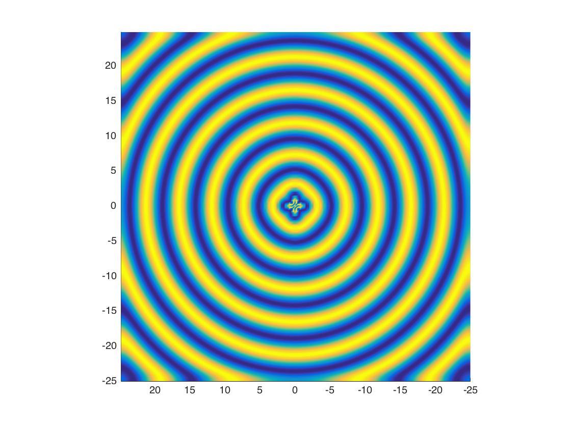
The matching procedure above relied strongly on the coupling kernels $\mathcal{L}$ and $J$ being local, and having a radial inhomogeneity $g(r)$, so the results do not immediately carry over to the case of nonlocal coupling and/or nonradial and algebraically localized inhomogeneities. Figure 1 depicts numerical results for particular cases of the nonlocal eikonal equation (2) given by

with $\varepsilon<0$ and $g(x,y)=(1+3x^{2}+y^{2})^{-3/2}$ in 1(a) and (b) (respectively $g(r,\theta)=(1+\cos(4\theta))/(1+r)^{3}$ in 1(c) and (d)). This evolution equation was integrated using a spectral discretization for the spatial operator and exponential time differencing (ETD) for the time stepping [CM02, KT05]. We will present a full discussion of our numerical methods and results in future work; here we only note that the far-field behavior of the target waves are (nearly) radially symmetric (see Figure 1) even in the general nonlocal problem. Indeed, setting $\partial_{t}\phi=-\omega$ with $\omega>0$, and rescaling to the “outer variables” $\tilde{x}=\sqrt{\omega}x,\tilde{y}=\sqrt{\omega}y$, we get $\tilde{\nabla}=\omega^{-1/2}\nabla,\tilde{\Delta}=\omega^{-1}\Delta$. Further, from the algebraic localization of $g$, it follows that

Consequently, the (formal) $\varepsilon\to 0$ limit equation in the outer variables is the viscous eikonal equation

This argument, together with the numerical results depicted in Figure 1, suggests that, even for general inhomogeneities, we may approximate the dynamics of target waves solutions in the outer region by a radial viscous eikonal equation

This intuition will guide our analysis of the nonlocal equation (2) for general coupling kernels and nonradially symmetric, algebraically localized perturbations $g$. We will show that the frequency indeed scales as $\omega\sim\exp\left(\frac{2}{\varepsilon M}\right)$, with $\varepsilon M<0$, and that the target waves that bifurcate from the steady state are radially symmetric far away from the inhomogeneity. Our strategy consists of first finding, in Section 4.2, solutions to equation (2), with $\omega=0$, which give the appropriate intermediate approximation. Then in Section 4.3 we find the “outer” solutions to equation (2) by treating the frequency $\omega$ as an extra parameter. Finally, in Section 4.4 we derive a relation between the frequency $\omega$ and the parameter $\varepsilon$ using asymptotic matching, and then proceed to prove the results of Theorem 1.

We define the Kondratiev space [McO79], $M^{s,p}_{\gamma}(\mathbb{R}^{d})$, with $d\in\mathbb{N},s\in\mathbb{N}\bigcup\{0\},\gamma\in\mathbb{R},p\in(1,\infty)$, as the space of locally summable, $s$ times weakly differentiable functions $u:\mathbb{R}^{d}\rightarrow\mathbb{R}$ endowed with the norm

From the definition, it is clear that these spaces admit functions with algebraic decay or growth, depending on the weight $\gamma$, and that these functions gain localization with each derivative. Moreover, given real numbers $\alpha,\beta$, such that $\alpha>\beta$, the embedding $M^{s,p}_{\alpha}(\mathbb{R}^{d})\subset M^{s,p}_{\beta}(\mathbb{R}^{d})$ holds, and additionally if $s$ and $r$ are integers such that $s<r$ then $M^{s,p}_{\gamma}(\mathbb{R}^{d})\subset M^{r,p}_{\gamma}(\mathbb{R}^{d})$. As in the case of Sobolev spaces, we may identify the dual $(M^{s,p}_{\gamma}(\mathbb{R}^{d}))^{*}$ with the space $M^{-s,q}_{-\gamma}(\mathbb{R}^{d})$, where $p$ and $q$ are conjugate exponents, and in the case when $p=2$ we also have that Kondratiev spaces are Hilbert spaces. In particular, given $f,g\in M^{s,2}_{\gamma}(\mathbb{R}^{d})$ the pairing

satisfies all the properties of an inner product. This is not hard to see once we notice that for every $f\in L^{2}_{\gamma}(\mathbb{R}^{d})$ the function $f({\bf x})\dot{(}1+|{\bf x}|^{2})^{\gamma/2}$ is in the familiar Hilbert space $L^{2}(\mathbb{R}^{d})$.

We will use this last property to decompose the space $M^{s,2}_{\gamma}(\mathbb{R}^{d})$ into a direct sum of its polar modes. Here we restrict ourselves to the case $d=2$ which is relevant for our analysis, but mention that a similar decomposition is possible in higher dimensions. More precisely, using the notation $M^{s,p}_{r,\gamma}(\mathbb{R}^{d})$ to denote the subspace of radially symmetric functions in $M^{s,p}_{\gamma}(\mathbb{R}^{d})$, we show that

The proof of this result follows the analysis of Stein and Weiss in [SW16].

We also have the following result describing how elements in $M^{1,2}_{\gamma}(\mathbb{R}^{d})$ decay at infinity (see Appendix B.1 for a proof).

In addition, the next lemma characterizes the multiplication property for Kondratiev spaces. The lemma is more general than we need in the sense that it holds for complete Riemannian manifolds that are euclidean at infinity, $(\mathbb{M},e)$. A proof of this result can be found in [CBC81]. We have adapted the notation so that it is consistent with our definition of Kondratiev spaces.

References

- [ADGK+08] Alex Arenas, Albert Díaz-Guilera, Jurgen Kurths, Yamir Moreno, and Changsong Zhou, Synchronization in complex networks, Physics reports 469 (2008), no. 3, 93–153.
- [AF03] Robert A Adams and John JF Fournier, Sobolev spaces, vol. 140, Academic press, 2003.
- [AK02] Igor S Aranson and Lorenz Kramer, The world of the complex Ginzburg-Landau equation, Reviews of Modern Physics 74 (2002), no. 1, 99.
- [AS92] Milton Abramowitz and Irene A. Stegun (eds.), Handbook of mathematical functions with formulas, graphs, and mathematical tables, Dover Publications Inc., New York, 1992, Reprint of the 1972 edition.
- [AT06] Igor S Aranson and Lev S Tsimring, Patterns and collective behavior in granular media: Theoretical concepts, Reviews of modern physics 78 (2006), no. 2, 641.
- [Boy99] John P. Boyd, The Devil’s invention: Asymptotic, superasymptotic and hyperasymptotic series, Acta Appl. Math. 56 (1999), no. 1, 1–98.
- [CBC81] Yvonne Choquet-Bruhat and Demetrios Christodoulou, Elliptic systems in spaces on manifolds which are Euclidean at infinity, Acta Mathematica 146 (1981), no. 1, 129–150.
- [CH93] M. C. Cross and P. C. Hohenberg, Pattern formation outside of equilibrium, Rev. Mod. Phys. 65 (1993), 851–1112.
- [CH09] Nicholas T. Carnevale and Michael L. Hines, The NEURON book, 1st ed., Cambridge University Press, New York, NY, USA, 2009.
- [CM02] S.M. Cox and P.C. Matthews, Exponential time differencing for stiff systems, J. Comput. Phys. 176 (2002), no. 2, 430–455.
- [Coo05] Stephen Coombes, Waves, bumps, and patterns in neural field theories, Biological cybernetics 93 (2005), no. 2, 91–108.
- [DSSS05] Arjen Doelman, Björn Sandstede, Arnd Scheel, and Guido Schneider, The dynamics of modulated wave trains, CWI. Modelling, Analysis and Simulation [MAS], 2005.
- [ER99] Jens Eggers and Hermann Riecke, Continuum description of vibrated sand, Phys. Rev. E 59 (1999), 4476–4483.
- [Erm98] Bard Ermentrout, Neural networks as spatio–temporal pattern–forming systems, Reports on progress in physics 61 (1998), no. 4, 353.
- [FB04] Stefanos E Folias and Paul C Bressloff, Breathing pulses in an excitatory neural network, SIAM Journal on Applied Dynamical Systems 3 (2004), no. 3, 378–407.
- [Fis37] R. A. Fisher, The wave of advance of advantageous genes, Annals of Eugenics 7 (1937), no. 4, 355–369.
- [Fit61] Richard FitzHugh, Impulses and physiological states in theoretical models of nerve membrane, Biophysical journal 1 (1961), no. 6, 445–466.
- [GJP+95] Richard A Gray, Jose Jalife, Alexandre V Panfilov, William T Baxter, Candido Cabo, Jorge M Davidenko, Arkady M Pertsov, Paulien Hogeweg, and Arthur T Winfree, Mechanisms of cardiac fibrillation, Science 270 (1995), no. 5239, 1222–1226.
- [GKS00] M. Golubitsky, E. Knobloch, and I. Stewart, Target patterns and spirals in planar reaction-diffusion systems, Journal of Nonlinear Science 10 (2000), no. 3, 333–354.
- [GSS88] Martin Golubitsky, Ian Stewart, and David Schaeffer, Singularities and groups in bifurcation theory : Volume II, Springer, New York, NY, 1988.
- [Hag81] Patrick S Hagan, Target patterns in reaction-diffusion systems, Advances in Applied Mathematics 2 (1981), no. 4, 400 – 416.
- [HTY+04] Xiaoying Huang, William C Troy, Qian Yang, Hongtao Ma, Carlo R Laing, Steven J Schiff, and Jian-Young Wu, Spiral waves in disinhibited mammalian neocortex, The Journal of Neuroscience 24 (2004), no. 44, 9897–9902.
- [Jar15] Gabriela Jaramillo, Inhomogeneities in 3 dimensional oscillatory media, Netw. Heterog. Media 10 (2015), no. 2, 387–399.
- [JS16] Gabriela Jaramillo and Arnd Scheel, Pacemakers in large arrays of oscillators with nonlocal coupling, Journal of Differential Equations 260 (2016), no. 3, 2060–2090.
- [JSW17] Gabriela Jaramillo, Arnd Scheel, and Qiliang Wu, The effect of impurities on striped phases, Proc. Roy. Soc. Edinb. (2017), to appear.
- [Kat13] Tosio Kato, Perturbation theory for linear operators, vol. 132, Springer Science & Business Media, 2013.
- [KB02] Yoshiki Kuramoto and Dorjsuren Battogtokh, Coexistence of coherence and incoherence in nonlocally coupled phase oscillators., Nonlin. Phenom. Comp. Sys. 5 (2002), no. 4, 380–385.
- [KB10a] Zachary P Kilpatrick and Paul C Bressloff, Effects of synaptic depression and adaptation on spatiotemporal dynamics of an excitatory neuronal network, Physica D: Nonlinear Phenomena 239 (2010), no. 9, 547–560.
- [KB10b] by same author, Spatially structured oscillations in a two–dimensional excitatory neuronal network with synaptic depression, Journal of computational neuroscience 28 (2010), no. 2, 193–209.
- [KH81] N Kopell and L. N Howard, Target pattern and spiral solutions to reaction–diffusion equations with more than one space dimension, Advances in Applied Mathematics 2 (1981), no. 4, 417–449.
- [KM04] Hiroshi Kori and Alexander S Mikhailov, Entrainment of randomly coupled oscillator networks by a pacemaker, Physical review letters 93 (2004), no. 25, 254101.
- [KPP37] Andrei Nikolaevitch Kolmogorov, Ivan G Petrovskii, and Nikolaï S Piskunov, A study of the equation of diffusion with increase in the quantity of matter, and its application to a biological problem, Bjul. Moskovskogo Gos. Univ (Bulletin Moscow State University) 1 (1937), no. 7, 1–26.
- [KS07] Richard Kollár and Arnd Scheel, Coherent structures generated by inhomogeneities in oscillatory media, SIAM Journal on Applied Dynamical Systems 6 (2007), no. 1, 236–262.
- [KT76] Yoshiki Kuramoto and Toshio Tsuzuki, Persistent propagation of concentration waves in dissipative media far from thermal equilibrium, Progress of Theoretical Physics 55 (1976), no. 2, 356–369.
- [KT05] A. Kassam and L. Trefethen, Fourth-Order time-stepping for stiff PDEs, SIAM Journal on Scientific Computing 26 (2005), no. 4, 1214–1233.
- [Kur75] Yoshiki Kuramoto, Self-entrainment of a population of coupled non-linear oscillators, International Symposium on Mathematical Problems in Theoretical Physics: January 23–29, 1975, Kyoto University, Kyoto/Japan (Huzihiro Araki, ed.), Springer Berlin Heidelberg, Berlin, Heidelberg, 1975, pp. 420–422.
- [Kur84] by same author, Chemical Oscillations, Waves, and Turbulence, Springer Series in Synergetics, vol. 19, Springer Berlin Heidelberg, Berlin, Heidelberg, 1984.
- [LT03] Carlo R Laing and William C Troy, PDE methods for nonlocal models, SIAM Journal on Applied Dynamical Systems 2 (2003), no. 3, 487–516.
- [McO79] Robert C McOwen, The behavior of the Laplacian on weighted Sobolev spaces, Communications on Pure and Applied Mathematics 32 (1979), no. 6, 783–795.
- [Mer92] Ehud Meron, Pattern formation in excitable media, Physics Reports 218 (1992), no. 1, 1–66.
- [MM95] Osamu Moriyama and Mitsugu Matsushita, Simple model for target patterns and spiral waves, Journal of the Physical Society of Japan 64 (1995), no. 4, 1081–1084.
- [Nag91] Hiroyuki Nagashima, Target patterns and pacemakersin a reaction–diffusion system, Journal of the Physical Society of Japan 60 (1991), no. 9, 2797–2799.
- [NAY62] Jinichi Nagumo, Suguru Arimoto, and Shuji Yoshizawa, An active pulse transmission line simulating nerve axon, Proceedings of the IEEE 50 (1962), no. 10, 2061–2070.
- [NW69] Alan C. Newell and J. A. Whitehead, Finite bandwidth, finite amplitude convection, J. Fluid Mech. 38 (1969), no. 2, 279–303.
- [PE01] David J Pinto and G Bard Ermentrout, Spatially structured activity in synaptically coupled neuronal networks: I. Traveling fronts and pulses, SIAM journal on Applied Mathematics 62 (2001), no. 1, 206–225.
- [PV87] A Pagola and C Vidal, Wave profile and speed near the core of a target pattern in the Belousov–Zhabotinsky reaction, Journal of Physical Chemistry 91 (1987), no. 3, 501–503.
- [RMO06] Filippo Radicchi and Hildegard Meyer-Ortmanns, Entrainment of coupled oscillators on regular networks by pacemakers, Physical Review E 73 (2006), no. 3, 036218.
- [ROH05] Juan G Restrepo, Edward Ott, and Brian R Hunt, Onset of synchronization in large networks of coupled oscillators, Physical Review E 71 (2005), no. 3, 036151.
- [Rou04] Violaine Roussier, Stability of radially symmetric travelling waves in reaction–diffusion equations, Annales de l’Institut Henri Poincare (C) Non Linear Analysis 21 (2004), no. 3, 341 – 379.
- [Seg69] Lee A. Segel, Distant side–walls cause slow amplitude modulation of cellular convection, J. Fluid Mech. 38 (1969), no. 1, 203–224.
- [Sim76] Barry Simon, The bound state of weakly coupled Schrödinger operators in one and two dimensions, Annals of Physics 97 (1976), no. 2, 279–288.
- [SK04] Shin-ichiro Shima and Yoshiki Kuramoto, Rotating spiral waves with phase–randomized core in nonlocally coupled oscillators, Physical Review E 69 (2004), no. 3, 036213.
- [SL12] Michael A. Schwemmer and Timothy J. Lewis, The Theory of Weakly Coupled Oscillators, Phase Response Curves in Neuroscience: Theory, Experiment, and Analysis (Nathan W. Schultheiss, Astrid A. Prinz, and Robert J. Butera, eds.), Springer New York, New York, NY, 2012, pp. 3–31.
- [SM06] Michael Stich and Alexander S Mikhailov, Target patterns in two–dimensional heterogeneous oscillatory reaction–diffusion systems, Physica D: Nonlinear Phenomena 215 (2006), no. 1, 38–45.
- [SW16] Elias M Stein and Guido Weiss, Introduction to Fourier analysis on Euclidean spaces, vol. 32, Princeton university press, 2016.
- [TF80a] John J Tyson and Paul C Fife, Target patterns in a realistic model of the Belousov–Zhabotinskii reaction, The Journal of Chemical Physics 73 (1980), no. 5, 2224–2237.
- [TF80b] John J. Tyson and Paul C. Fife, Target patterns in a realistic model of the Belousov-Zhabotinskii reaction, The Journal of Chemical Physics 73 (1980), no. 5, 2224–2237.
- [UMS98] Paul B. Umbanhowar, Francisco Melo, and Harry L. Swinney, Periodic, aperiodic, and transient patterns in vibrated granular layers, Physica A: Statistical Mechanics and its Applications 249 (1998), no. 1–4, 1–9.
- [VO98] Shankar C. Venkataramani and Edward Ott, Spatiotemporal bifurcation phenomena with temporal period doubling: Patterns in vibrated sand, Phys. Rev. Lett. 80 (1998), 3495–3498.
- [VO01] by same author, Pattern selection in extended periodically forced systems: A continuum coupled map approach, Phys. Rev. E 63 (2001), 046202.
- [Win73] Arthur T. Winfree, Scroll-Shaped waves of chemical activity in three dimensions, Science 181 (1973), no. 4103, 937–939.
- [WW96] E. T. Whittaker and G. N. Watson, A course of modern analysis, Cambridge Mathematical Library, Cambridge University Press, Cambridge, 1996, Reprint of the fourth (1927) edition.
- [YHLZ13] Nan Yao, Zi-Gang Huang, Ying-Cheng Lai, and Zhi-Gang Zheng, Robustness of chimera states in complex dynamical systems, Scientific reports 3 (2013), 3522.