∎
Energy preserving model order reduction of the nonlinear Schrödinger equation
Abstract
An energy preserving reduced order model is developed for two dimensional nonlinear Schrödinger equation (NLSE) with plane wave solutions and with an external potential. The NLSE is discretized in space by the symmetric interior penalty discontinuous Galerkin (SIPG) method. The resulting system of Hamiltonian ordinary differential equations are integrated in time by the energy preserving average vector field (AVF) method. The mass and energy preserving reduced order model (ROM) is constructed by proper orthogonal decomposition (POD) Galerkin projection. The nonlinearities are computed for the ROM efficiently by discrete empirical interpolation method (DEIM) and dynamic mode decomposition (DMD). Preservation of the semi-discrete energy and mass are shown for the full order model (FOM) and for the ROM which ensures the long term stability of the solutions. Numerical simulations illustrate the preservation of the energy and mass in the reduced order model for the two dimensional NLSE with and without the external potential. The POD-DMD makes a remarkable improvement in computational speed-up over the POD-DEIM. Both methods approximate accurately the FOM, whereas POD-DEIM is more accurate than the POD-DMD.
Keywords:
Nonlinear Schrödinger equation Discontinuous Galerkin method Average vector field method Proper orthogonal decomposition Discrete empirical interpolation method Dynamic mode decompositionMSC
MSC 65P10, 65M60, 365Q55, 37M15, 93A151 Introduction
The nonlinear Schrödinger equation (NLSE) is used frequently for modelling wave propagation phenomena in different areas of physics, chemistry and engineering. In quantum physics and chemistry, the NLSE is used in the study of Bose-Einstein condensation (BEC), where it is also called Gross-Pitaevskii equation (GPE). The numerical simulations are extremely important for predicting the long term behavior of NLSE/GPE, because experiments to create BECs are challenging and computationally expensive.
The structure preserving symplectic and multisymplectic [14, 22, 35] integrators and energy preserving integrators [18] using finite difference discretization in space, lead to long term stability of the solutions of Hamiltonian partial differential equations (PDEs) like the NLSE. In [44] local energy-preserving multi-symplectic algorithms in time are constructed for coupled and two dimensional NLSE using pseudospectral methods or Gauss-Legendre collocation methods for the spatial discretization.
Due to the implicit nature of these integrators, at each time step, a coupled fully nonlinear system has to be solved by a fixed point or a Newton-Raphson method with high accuracy [33]. The discrete energy is conserved when the nonlinear system is solved accurately up to the machine precision. Therefore solving NLSE might be extremely time consuming, especially for two and three dimensional (2D and 3D) problems.
The goal of this work is fast and accurate reduced order modeling for the 2D NLSE that preserves energy and mass. The proper orthogonal decomposition reduced order model (POD-ROM) has been widely used as a computationally efficient surrogate model in large-scale numerical simulations of complex systems. However, when it is applied to a Hamiltonian system like the NLSE, naive application of the POD method can destroy the Hamiltonian structure in the reduced order model. The stability of reduced models over long-time integration and the structure preserving properties has been recently investigated in the context of Lagrangian systems [43, 16], and for Hamiltonian systems [12, 20]. For linear and nonlinear Hamiltonian systems, a symplectic model reduction technique, proper symplectic decomposition (PSD) with symplectic Galerkin projection is constructed in [49] which captures the symplectic structure of Hamiltonian systems to ensure long term stability of the reduced model. The PSD is computed using three algorithms; complex SVD, cotangent lift and nonlinear programming. The PSD-DEIM method is extended with a greedy algorithm to parametric Hamiltonian systems in [1]. For nonlinear Hamiltonian systems, the PSD is combined with the discrete empirical interpolation method (DEIM) to reduce the computational cost [49, 1]. Recently the energy preserving average vector field (AVF) method is used as a time integrator to construct reduced order models for Hamiltonian systems [31], for dissipative gradient systems like the Allen-Cahn equation [57]. In general, there exist no numerical integration method that preserves both the symplectic structure and the energy of a Hamiltonian systems. The snapshots are enriched using the gradients of the Hamiltonian at time instances in [31]. Besides the symplectic [33] and multi-symplectic structure preserving geometric integrators [14], there are energy or Hamiltonian preserving integrators; the average vector field (AVF) method [51, 18]. The AVF is second order convergent in time, and preserves the time reversal symmetry of the Hamiltonian systems like the implicit mid-point rule. Energy preservation of various PDEs by the AVF method is studied in [18]: Hamiltonian and dissipative PDEs, like the NLSE, Korteweg-de Vries equation, Sine-Gordon equation, Allen-Chan equation, Ginzburg Landau equation and Maxwell equation.
Currently the symplectic and energy preserving reduced order models are applied to one dimensional linear and non-linear Hamiltonian systems using finite differences in space; linear wave equation [49, 1, 31], NLSE [49, 1], Sine-Gordon equation [49], Korteweg-de Vries equation [31]. The long term computation of the two dimensional NLSE with and without external potential is computationally challenging and more expensive than the one dimensional NLSE. In this paper we develop an energy stable reduced order model (ROM) for two dimensional NLSE, which inherits the energy preservation property of the full order model (FOM). For the space discretization we apply symmetric interior penalty discontinuous Galerkin (SIPG) method [8, 52], and for time discretization the energy preserving AVF method. The SIPG is more efficient by evaluations of the nonlinear terms than the continuous FEM [38]. The AVF method preserves the energy dissipation of gradient systems like the Allen-Cahn equation [39] and the skew-gradient structure like the diffusive FitzHugh-Nagumo equation [38]. Reduced order models, which preserve the energy dissipation of gradient and skew-gradient systems are developed in [38, 57]. The POD-Galerkin approach involves an offline-online splitting methodology. In the offline stage, the high fidelity or truth solutions are generated by numerical simulations of the discretized high dimensional FOM. The POD is then applied to compute an optimal subspace to fit the high fidelity data. A reduced system is constructed by projecting the high-dimensional system to this subspace. In the online stage, the reduced system is solved in the low-dimensional subspace. The primary challenge in producing the low dimensional models of the high dimensional discretized PDEs is the efficient evaluation of the nonlinearities (inner products) on the POD basis. Different POD Galerkin methods are developed to reduce the complexity of evaluating the nonlinear terms; gappy POD [27, 15], missing point estimation [9, 63], empirical and discrete empirical interpolation method (EIM/DEIM) [11, 21]. Recently the dynamic mode decomposition (DMD) has appeared as an alternative to produce low rank approximation of the nonlinear terms [3]. Like the DEIM, the DMD uses singular value decomposition (SVD) of the nonlinearities, which also uses sparse sampling through the gappy POD and DEIM/EIM. In [60] a hybrid combination of the POD with DMD is applied to the one dimensional NLSE and to the Ginzburg-Landau equation. Recently in [19], for the incompressible Navier-Stokes equation (NSE), energy, mass and angular momentum conserving Galerkin discretization methods are developed in convective, skew-symmetric, conservative, and rotational formulations. The conservation properties of ROMs such as energy balance and mass conservation for the NLSE are investigated theoretically and numerically [48].
Efficient computation of the reduced order basis functions is an important aspect in reduced order modelling. The reduced order basis functions in POD-DEIM and POD-DMD are computed in the offline stage using singular value decomposition (SVD), which can be computationally demanding for large snapshot matrices. Here we use the randomized singular value decomposition (rSVD) [34, 45, 46] as a fast and accurate alternative to the deterministic SVD to reduce the computational cost in the offline stage [2, 13, 26]. We compare the DEIM and DMD with respect to the accuracy and efficiency. We show that ROMs preserve well the energy and mass of the FOMs through numerical simulations for two dimensional NLSE with and without an external potential. It turns out that POD-DMD is several orders faster than the POD-DEIM, but less accurate than the POD-DEIM.
The remainder of the paper is organized as follows. The NLSE is reviewed briefly in Section 2. Space-time discretization of NLSE by the SIPG and AVF method is given in Section 3. In Section 4, the energy preserving ROM, and also the POD-DEIM and POD-DMD are presented. The preservation of the invariants like the energy and mass of the NLSE, efficiency and accuracy of the ROMs are illustrated through the numerical simulations in Section 5. The paper ends with some conclusions.
2 Nonlinear Schrödinger equation
The general form of the NLSE equation with a cubic nonlinearity and an external potential is given by
| (1) |
with an initial condition
| (2) |
where is the complex valued wave function, is the complex unity (), is the Laplace operator, is the time variable, is a terminal time, is a positive constant, and is a bounded polygonal computational domain. In this paper we consider two dimensional () NLSE, and we set the spatial variable . The parameter is a dimensionless constant with negative value for focusing (or attractive) and positive value for defocusing (or repulsive) nonlinearity. The external potential function is a given real-valued function and its specific form depends on different applications [50, 55]. For BEC, it is usually chosen as a harmonic confining potential, i.e., quadratic polynomial [5, 10]. The boundary conditions are usually of homogeneous Dirichlet or periodic type. We consider here periodic boundary conditions in the space time domain
For the NLSE (1), we relate the mass (or density) functional and the energy functional , given as usual by
| (3a) | ||||
| (3b) | ||||
The NLSE (1) is a Hamiltonian PDE which is well-known for Hamiltonian PDEs [55, 10] that it conserves the mass (3a) and the energy (3b) as the time progresses, in other words, the mass and energy at all times is equal to the mass and energy at the initial time :
| (4) |
with the initial condition .
There are other important dynamical properties of the solution to the NLSE (1); time reversibility or symmetry, time transverse or gauge invariance, dispersion relation for NLSE without external potential. The Gross-Pitaevskii equation (GPE) is NLSE for the macroscopic wave functions, governs the properties of BECs at temperatures far below the critical condensation temperature. The GPE includes the external potential term.
There exists a huge literature for the numerical solution of the NLSE, especially for 1D problems. Numerical methods for 2D NLSE include the alternating direction implicit (ADI) method [62], implicit-explicit multistep method [29], high order compact finite difference schemes [59], and local discontinuous Galerkin method [61], the implicit Crank-Nicolson finite difference (CNFD), semi-implicit finite difference (SIFD), time splitting spectral and pseudo spectral methods [6, 7].
3 Full order model
In this section we introduce the space-time discretization of the NLSE (1) leading to the so-called full order model (FOM), and we discuss the preservation of invariants for FOM under symmetric interior penalty Galerkin (SIPG) space discretization together with average vector field (AVF) time integrator.
Applying Green’s formula to the NLSE (1), the continuous weak formulation of the problem (1) can be written as follows: for a.e. , find such that for any
| (5a) | |||||
| (5b) | |||||
where denotes the -inner product on the space of square integrable functionals over a domain , and together with the corresponding norm :
The solution space is set as the space of functions in the Sobolev space satisfying the periodicity on the boundary of the domain :
We decompose the complex valued wave function into its real and imaginary parts as , then (5) can be re-written as a pair of real-valued system:
| (6a) | |||||
| (6b) | |||||
| (6c) | |||||
where . In the following, we introduce the SIPG method [8, 52] for the spatial discretization of NLSE. We remark that among the three common interior penalty Galerkin discretizations, nonsymmetric interior penalty Galerkin (NIPG), and incomplete interior penalty Galerkin (IIPG), only SIPG leads to a Hamiltonian system of ODEs [36].
3.1 Semi-discretization in space
Consider for , as a family of shape-regular simplicial triangulations of . Each mesh consists of closed triangles such that holds. The diameter of an (triangular) element and the length of an edge are denoted by and , respectively. We split the set of all edges into the set of interior edges and the set of periodic boundary edge-pairs. An individual element of the set is of the form where , and is the corresponding periodic edge-pair of with . Let the edge be a common edge for two elements and . For a piecewise continuous scalar function , there are two traces of along , denoted by from inside and from inside . Then, the jump and average of across the edge are defined by:
where (resp. ) denotes the unit outward normal to (resp. ). Similarly, for a piecewise continuous vector field , the jump and average across the edge are given by
For a boundary edge , we set and , where is the unit outward normal vector to . The treatment of the periodic boundary edges is the same as the interior edges, in other words, appropriate jump and average operators introduced in [58] are used. Then, for each , we define the jump and average operators as follow
where, for , we use the fixed unit outward normal vector to the boundary edge .
For continuous finite elements methods (FEMs), the idea is to approximate the solutions and of (6) from a conforming, finite dimensional space . On the other hand, we point out that in discontinuous Galerkin (dG) methods the space of solutions or test functions consist of piecewise discontinuous polynomials. That is, no continuity constraints are explicitly imposed on the state and test functions across the element interfaces. As a consequence, weak formulations must include jump terms across interfaces, and typically penalty terms are added to control the jump terms. We define the space of solution and test functions by
| (7) |
where is the set of polynomials of degree at most in . Note that the space of discrete solutions and the space of test functions are identical due to the weak treatment of boundary conditions in dG methods. Note also that the space is a non-conforming space, i.e., .
Let be the projections (orthogonal -projection) of the initial conditions and onto , i.e.,
| (8) |
Then, the weak formulation of the system (6), discretized by the SIPG method, reads as: for a.e. , find , such that
| (9a) | |||||
| (9b) | |||||
where the bi-linear form and the non-linear forms for are given for any by
where the parameter in the above formulation is called penalty parameter which should be sufficiently large to ensure the stability of the SIPG discretization with a lower bound depending only on the polynomial degree , see, e.g., [52].
The SIPG discretized semi-discrete solutions of (9) are given as
| (11) |
where , and are the unknown coefficients and the basis functions for , respectively, for and . The number denotes the number of (triangular) elements in , and is the local dimension on each element with the identity for the 2D problems , where is the degree of the polynomial order. Note that the degrees of freedom in dG methods are given by , and throughout this paper we denote by the dimension of the high-fidelity model, i.e., the full order model (FOM). Inserting the expansions (11) into the system (9), we obtain the following semi-discrete Hamiltonian system
| (12) |
where , and and are the unknown coefficient vectors for the solutions and with the ordered entries
The other settings are given by
| (13) |
where is the usual mass matrix, is the stiffness matrix corresponding to the bilinear form , and are the vectors corresponding to the non-linear forms (inner products) for . The matrix is the skew-symmetric matrix with Id is the dimensional identity matrix.
3.2 Time discretization
For the temporal discretization of the semi-discrete system (12), we use the energy preserving, implicit, second order convergent AVF method [18, 51]. For a system of ordinary differential equations (ODEs)
the AVF method reads as
where is the unknown solution at time , is the known solution at time , and is the uniform time-step size. The AVF method also preserves the energy of Hamiltonian systems and Poisson systems with non-constant skew-symmetric structure [33], like the KdV equation and bi-Hamiltonian systems [37]. For problems with polynomial Hamiltonians, the AVF method can be interpreted as the Runge–Kutta method [17], where the integrals can be evaluated exactly, and the implementation is comparable to that of the implicit mid-point rule. Using the multi-symplectic formulation of Hamiltonian PDEs, the AVF method is applied as an energy-preserving wavelet collocation to the NLSE and Camassa-Holm equation [32], and as local energy-preserving method to the NLSE and KdV equation [30], to the 2D NLSE [44].
For time discretization, we divide the time interval into steps: with the uniform time step size , . We set as the approximate solution vector at the time instance , , with , and and . For , let be the projections (orthogonal -projections) of the initial conditions onto , and let and be the corresponding initial coefficient vectors satisfying the expansions (11), and set . Then, applying the AVF method to the semi-discrete system (12), the full discrete problem of the NLSE (1) reads as: for , find satisfying
3.3 Preservation of the invariants in FOM
The NLSE is time reversible or symmetric, i.e., the solutions are unchanged under the change of time as and taken conjugate in the equation (1). For the full discrete scheme, the time reversibility implies that the scheme remains unchanged under the operation: and which is also true for the midpoint rule (Crank-Nicolson finite difference scheme) [5] and SIPG-AVF scheme. There are two other invariants. The first one is the time transverse or gauge invariance, i.e., the translation of the potential changes the phase of the solution as . The density or modulus of the solutions, , is unchanged. NLSE admits plane wave solutions, satisfying a dispersion relation. NLSE without external potential (when ) generates plane wave solutions , where is the amplitude, is the time frequency, is the spatial wave number. Like the Crank-Nicolson method, AVF method can not preserve the time translation invariant and the dispersion relation. For an overview of the preservation of invariants of NLSE at the discrete level and computational cost we refer to [5].
In the sequel, we show the conservation of discrete mass and discrete energy.
Theorem 3.1
The semi-discrete solution through the FOM (12), discretized by the SIPG method, conserves the discrete mass
| (14) |
exactly for all time.
Proof
To prove the discrete mass conservation, we utilize the weak formulation (9) of FOM. We choose the test functions in (9a) and in (9b). Then, summation of (9a) and (9b), and using the linearity of bilinear form in both arguments, yields
by which we obtain
From this equation we can see that the discrete mass is invariant for all time. ∎
For the discrete energy preservation, we first introduce the following mesh-dependent energy functional which can be regarded as SIPG counterpart of the continuous energy functional defined in (3b):
| (15) |
where
Note that for a continuous solution , since , we have .
Theorem 3.2
The FOM (12) is a Hamiltonian ODE
Proof
Firstly, we claim that , for which then (16) is the FOM (12). For this, by the definition of the bilinear form in (10), note that the discrete energy functional in (15) can be written as
| (17) |
Then, Fréchet derivatives of with respect to the components and in any directions are:
or in matrix-vector form
Hence, with the definition of the matrices and vectors in (13), we obtain that
| (18) |
Further, using the identity (18) and the FOM (12), the invariance of the energy for all time follows as:
since the matrix is again a skew-symmetric matrix due to the fact that is a skew-symmetric matrix and is symmetric.∎
4 Reduced order model
Because the computation of the FOM (12) is time consuming, in this section, we construct a small dimensional reduced order model (ROM) by utilizing the proper orthogonal decomposition (POD) method [41]. In addition to POD, the nonlinear vectors in the ROM are computed efficiently by discrete empirical interpolation method (DEIM) and dynamic mode decomposition (DMD). The low-rank approximation is computed in three steps: computation of the numerical solutions of the original high-dimensional system; dimensionality-reduction of the snapshot matrices by singular value decomposition (SVD); Galerkin projection of the dynamics on the low-rank subspace. The first two steps are known as the offline stage, and the last one is the online stage. Offline stage is usually expensive and online step should be fast to run in real time.
4.1 POD Galerkin projection
For the -dimensional FOM (12), the ROM of lower dimension is formed by the Galerkin projection of the system onto a -dimensional reduced space
resulting in the lower dimensional reduced solution as:
| (19) |
where, without lost of generality, we have assumed that the complex solution is the column vector of the real and imaginary solutions and , respectively, i.e., , by which the solution of the FOM (12) becomes the dG coefficient vector of at time . From the coefficients in (19), we set the solution of the reduced system as . The functions in (19) are the orthogonal (in -sense) reduced basis functions spanning the reduced space . Belonging to the space , the reduced basis functions are linear combination of the dG basis functions , given by
Then, using the column vectors , which are the coefficients of the -th reduced basis function, we construct the following matrix of POD modes
| (20) |
To obtain the reduced basis functions , we need to solve the minimization problem [41]
where is the Kronecker delta. The above minimization problem is equivalent to the eigenvalue problem [41]
| (21) |
where is the snapshot matrix whose -th column vector is the solution vector of the FOM at time . Then, the matrix of POD modes can be computed through the singular value decomposition (SVD) of the snapshot matrix . In addition, between the solution vector of FOM and the reduced solution vector of ROM, we have the relation
from where we can find the initial reduced vector . For a more detail description, we refer to [38]. We finally obtain the following reduced system:
| (22) |
with the reduced stiffness matrix and the reduced nonlinear vector
4.2 Randomized singular value decomposition
The SVD is known to be computationally demanding for large snapshot matrices resulting from the space-time discretized high dimensional model of the PDEs. Recently randomized algorithms are used in reduced order modelling to accelerate the offline computations in DMD [2, 13, 26]. Randomized methods for matrix computations provide an efficient computation of low-rank structures in data matrices, which are robust, reliable and computationally efficient and can be used to construct a smaller (compressed) matrix, which accurately approximates a high-dimensional data matrix. The randomized singular value decomposition (rSVD) is robust, reliable and computationally efficient, which approximates the high dimensional snapshot matrices by constructing a smaller (compressed) matrix [34, 45, 46].
Given a snapshot matrix and the target rank , a low rank approximation is constructed by creating a random matrix , then the sampled matrix . The entries of the random sampling matrix are independent and identically distributed Gaussian random variables of zero mean and unit variance [2], and they are created by the MatLab routine randn. Afterward the decomposition of is computed to obtain the orthonormal matrix , , so that
is satisfied. In the last step, the SVD of the small (compressed) matrix is computed. The approximation error of the rSVD can be decreased by introducing a small oversampling parameter (e.g. ). Instead of random vectors, are generated.
We use the rSVD for the SVD computations required in the POD reduced basis calculations, and the DEIM and DMD reduced basis calculations of the nonlinear terms.
4.3 Preservation of the invariants in ROM
In this section we show the preservation of discrete mass and discrete energy for the ROM (22). While the former is not difficult to show, we should state additional modifications to show the discrete energy preservation in ROM.
Proof
The proof of the mass conservation in ROM follows very similar to the proof for the FOM in Theorem 3.1. But now, we consider the weak formulation not on the space of dimension but on the reduced space . ∎
Theorem 4.2
The ROM (22) with the discrete energy defined in (15), does not necessarily satisfy the invariance of the discrete energy for all time. But the updated ROM
| (23) |
with the updated reduced matrix and the updated reduced vector , where the skew-symmetric matrix is such that , preserves the energy for all time.
Proof
| (24) |
Then, for the discrete energy functional of the reduced system, we have that
which may be non-zero since the matrix is not necessarily a skew-symmetric matrix. But, if we can find a skew-symmetric matrix so that , then we can obtain an equivalent equation of the updated ROM (23) as
| (25) |
The equation (25), as a result the updated ROM (23), is now Hamiltonian since is skew-symmetric. Then, we also get for the discrete energy functional that
Hence the ROM (23) satisfies the invariance of the discrete energy for all time. Indeed, the skew-symmetric matrix can be easily computed as
where we used the -orthogonality of the POD modes , i.e., . ∎
Remark 1
The preservation of the reduced energy is valid for any reduced Hamiltonian system of ODEs (23).
4.4 Approximation of the nonlinearities
Although the reduced model (23) is of small dimension, the computation of the nonlinear vector still depends on the dimension of the FOM. In this section, we give two different approaches to reduce the computational complexity due to the nonlinear vector in the ROM (23): discrete empirical interpolation method (DEIM) [21] and dynamic mode decomposition (DMD) [2, 3].
4.4.1 Discrete empirical interpolation method (DEIM)
The DEIM aims to find an approximation to the nonlinear vector , full dimensional nonlinear part of the reduced nonlinear vector , by projecting it onto a subspace of the space generated by the non-linear vectors and spanned by a basis of dimension :
| (26) |
where is the DEIM basis matrix, and is the corresponding coefficient vector. Since the system (26) is overdetermined, a projection matrix with is the -th column of the identity matrix is computed. Then, the reduced model (23) can be rewritten as:
| (27) |
where the matrix is computed once in the off-line stage (finite element discretization), and the reduced nonlinear vector requires only integral evaluations. Using the definition of reduced matrix , we also have an equivalent formulation of (27) that
| (28) |
where is the DEIM approximation of the nonlinear part . When DEIM approximation is not used, it requires integral evaluations. On the other hand, the computation of the Jacobian of the nonlinear vector requires integral evaluations without DEIM, but it is only with DEIM approximation.
For the details of the computation of the reduced non-linear vectors we refer to the greedy DEIM algorithm [21]. For continuous finite element and finite volume discretizations, the number of flops for the computation of bilinear form and nonlinear term depends on the maximum number of neighbor cells [25]. In the case of dG discretization, due to its local nature, it depends only on the number of nodes in the local cells. For instance, in the case of SIPG with linear elements (), it contributes only 3 nonzero integrals for each degree of freedom, hence 3 integrals have to be computed on a single triangular element [38], whereas in the case of continuous finite elements, integral computations on neighbor cells are needed [4]. Since the AVF method is an implicit time integrator, at each time step, a non-linear system of equations has to be solved by Newton’s method. The reduced Jacobian has a block diagonal structure for the SIPG discretization, which is easily invertible [38], and requires only operations with DEIM.
Because the nonlinearity in the ROM (23) is approximated by DEIM, the discrete energy is also preserved approximately in (27), not exactly as for the ROM (23), since we have that
But an upper bound for the preservation of the discrete energy by POD-DEIM can be derived as follows:
where in the last row, we have added which does not affect the identity since . Using that , we obtain
| (29) |
Finally, using the DEIM approximation error (21, Lemma 3.2)
we obtain an upper bound for the change of the energy with respect to time:
4.4.2 Dynamic mode decomposition (DMD)
The DMD extracts dynamically relevant spatio-temporal information content from a numerical or experimental data sets [42]. It is a powerful equation-free, data-driven method to analyze complex systems. Without explicit knowledge of the dynamical system, the DMD algorithm determines eigenvalues, eigenmodes, and spatial structures for each mode. The order of orthogonal POD modes are decreasing by the energy level of POD singular values. The DMD modes are not orthogonal and each DMD mode is associated with a growth rate and each mode has a single frequency. Again the DMD modes are ordered in form of decreasing energy; unlike the POD modes, they give the energy fluctuations at different frequencies. After building the DMD basis functions of rank , we approximate the full dimensional nonlinear part of the nonlinear term in (23) following [2, 3].
DMD is a special case of the Koopman operator [40] approximating nonlinear systems via an associated infinite dimensional system. The connection between the DMD and Koopman operator was established in [47, 53, 54] . The Koopman operator acts on a set of scalar observable functions
for the nonlinear dynamical system
| (31) |
where , an n-dimensional manifold. The DMD determines the Koopman eigenvalues and modes directly from the data, when the observable is considered as state space, . For construction of the DMD modes, we follow (Chapter 1,[42] ). The nonlinear system (31) is approximated locally by the following linear system
| (32) |
by constructing the discrete dynamical system
for trajectories, and . Low rank eigen-decomposition of the matrix is constructed by minimizing
| (33) |
in the least squares sense for all trajectories . For minimization of the approximation error (33), we consider the snapshot matrices and formed as:
Then, we find the unknown matrix satisfying , which is the solution of the minimization problem in the Frobenius norm
so that , where denotes the Moore-Penrose pseudo inverse. The DMD modes are computed by the exact DMD algorithm [56].
In our case, the exact DMD algorithm, Algorithm 2, is applied to the snapshot matrices and formed by the snapshots of the nonlinear terms in the FOM (12) at equally spaced time instances as:
Then, we obtain the time dependent DMD approximation to the nonlinear part in the ROM (23) as
| (34) |
where are DMD basis functions of rank of the nonlinear vector , is the initial vector and , . After plugging this term into (23), we obtain the following linear ROM:
| (35) |
The POD-DMD ROM (35) corresponds to the semi-discretized linear Schrödinger equation with an additional time dependent term coming from the linearization by POD-DMD approximation. The reduced energy of the POD-DMD contains only quadratic terms in (3b) like linear Schrödinger equation [24]. The AVF method is equivalent to the midpoint rule for quadratic potentials which is also energy preserving [18, 23]. Because the POD-DMD approximation of the cubic nonlinearity of the NLSE is reduced to a time dependent function appearing as additional term in the linear Schrödinger equation, the mass and energy are preserved with a lower accuracy than by POD-DEIM, which is shown by the numerical results in the next section. Although the dimension of the system (35) is the same as (27), the main advantage of the system (35) is that it is linear and we do not need to use the Newton’s method. Therefore the POD-DMD is significantly much faster than POD and POD-DEIM.
5 Numerical results
In this section we present numerical results for the NLSE (1) on a 2D localized rectangle with periodic boundary conditions. In all simulations we use linear dG basis functions on a uniform rectangular grid with triangular elements. Because the NLSE generate wave type solutions, it is not possible to capture the dynamics with few modes. For numerical simulations, the number of POD modes are fixed according to the relative information content or energy criterion given by
| (36) |
where is the -th singular value in the SVD of the snapshot matrix for computing the matrix of POD modes, and is the rank of the snapshot matrix . We set the number of POD modes as which sufficiently reflects the system characteristics. In the POD and DEIM/DMD modes computation procedure, we use rSVD algorithm, Algorithm 1, for the computation of SVD with the random matrix and the oversampling parameter . In all numerical experiments we have used for the FOM and ROMs the same time-step sizes. All simulations are performed on a Windows 10 machine with Intel Core i7, 2.5 GHz and 8 GB using MATLAB R2014.
5.1 Defocusing NLSE with progressive wave solutions
where and . The initial data is evaluated by taking using the exact solution. Numerical solutions are obtained with the linear dG elements in the spatial domain and for the final time , with the spatial and temporal mesh sizes and , respectively. The parameter values are taken as , and .
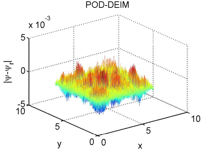
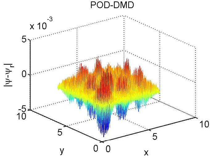
In Fig. 1 the decay of singular values are shown for the snapshot matrices of the solutions and nonlinear terms. At the very beginning a steep decay of singular values is observed. With increasing number of the modes, the singular values decay rather slowly. We choose in the ROM the number of POD modes which satisfies the energy criterion (36) with . In Fig. 2 the FOM solution and the errors between FOM and ROMs are shown at the final time. The number of DEIM and DMD modes are chosen to obtain the same level of accuracy for the error between the FOM and ROM solutions [3]. Both POD-DEIM and POD-DMD approximations with 15 DEIM/DMD modes for 10-rank truncation (POD modes) have almost the same accuracy.

In Fig. 3, the energy and mass errors are shown for the FOM and the ROM in -norm. The ROM errors are larger than the FOM errors as expected, but both mass and energy are well preserved.
On the other hand, for fixed number of POD modes , the relative errors of the solution, of the discrete energy and of the discrete mass in Fig. 4 decay monotonically with increasing number of the DEIM/DMD modes, and after they stagnate. Similar results were obtained for 1D NLSE in [3].
It can be clearly seen from Table 1 that the POD-DMD is much faster than the POD-DEIM, whereas there is no significant difference in the relative errors in Fig. 4. The advantage of the DMD lies in the fact that the ROM becomes linear, whereas in the case of DEIM, the ROM is still semi-linear and the nonlinearity have to be evaluated.
| CPU Time (sec.) | Speedup | |
|---|---|---|
| FOM | 8024.7 | - |
| ROM with DEIM | 763.9 | 10.5 |
| ROM with DMD | 8.2 | 974.3 |
In Fig. 5, we give the discrete energy and the discrete mass errors for the ROMs in -norm, using a larger time-step size than for the FOM. The discrete energy and the discrete mass are still preserved but with a lower accuracy.
We show in Figure 6 that the discrete energy and the discrete mass are not conserved when a non-conservative time integrator like the backward Euler method is used.
5.2 NLSE with an external potential
The initial data is taken as the Gaussian
in the space-time domain and , with the uniform spatial and temporal mesh sizes and , respectively. The diffusion constant is set as . The decay of the singular values in Fig. 7 is similar to the previous Example, i.e. NLSE without the external potential.
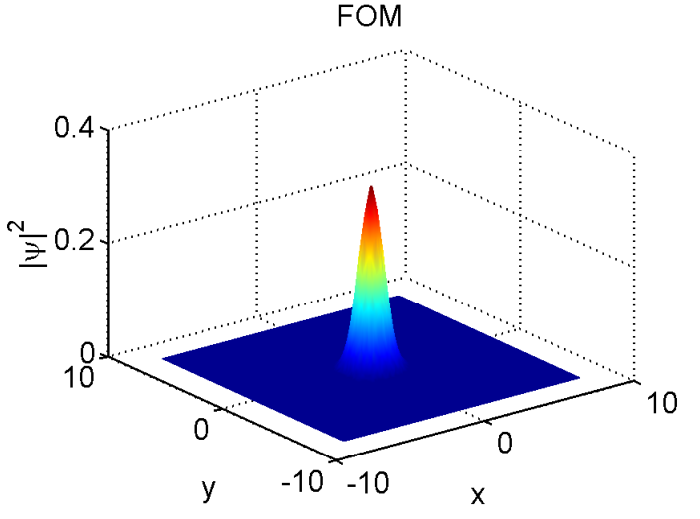
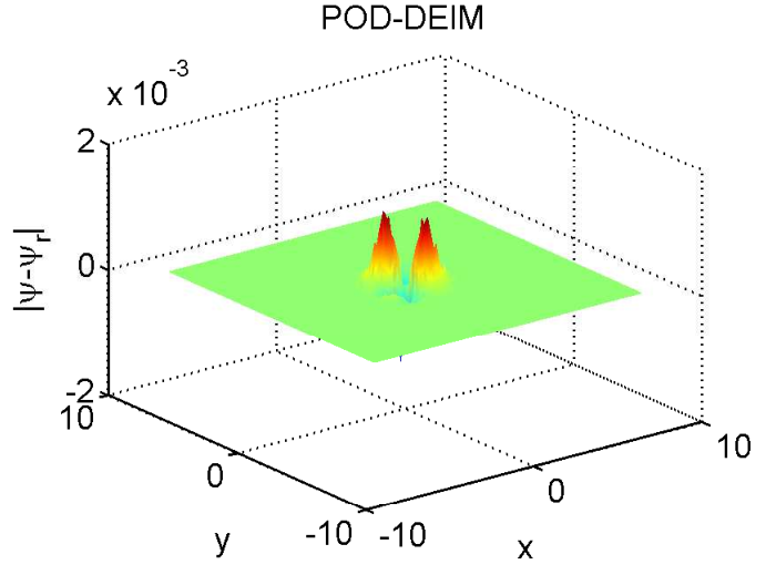
The POD-DEIM and POD-DMD solutions in Fig. 8 have again the same accuracy, but requiring more POD, DEIM and DMD modes than the NLSE without the external potential. We set the number of POD modes according to the energy criterion , further increase would not contribute a valuable accuracy.
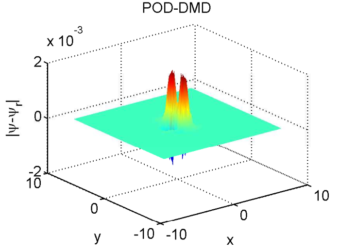
Again the discrete energy and the discrete mass are well preserved in Fig. 9 by the FOM and the ROMs.
The solution, discrete energy and discrete mass errors in Fig. 10 reach a plateau by increasing number of DEIM/DMD modes, and the POD-DEIM is much more accurate than the POD-DMD. The computational efficiency of the ROM with the DMD is clearly seen in Table 2. Similar results are obtained for the one dimensional Burger’s equation and NLSE in [3].
| CPU Time (sec.) | Speedup | |
|---|---|---|
| FOM | 309.7 | - |
| ROM with DEIM | 27.5 | 11.3 |
| ROM with DMD | 0.3 | 956.7 |
6 Conclusions
We have performed a comparative study using the energy preserving ROM applied to 2D NLSE, showing the numerical efficiency and accuracy of the reduced order approximations and the complexity reduction of the nonlinear terms with DEIM and DMD. The discrete energy and the discrete mass preservation of POD-DEIM and POD-DMD reduced order models have been shown to be accurate and efficient for capturing the spatio-temporal dynamics of the 2D NLSE with substantial reduction in both dimension and computational time. This is clearly demonstrated in numerical simulations by the comparative computation times (speed-ups) and relative errors of the reduced order systems with respect to FOMs. The POD-DMD is always faster and the POD-DEIM is in general more accurate.
Acknowledgments: The authors would like to thank the reviewers for the comments and suggestions that helped to improve the manuscript.
References
- (1) Afkham, B.M., Hesthaven, J.S.: Structure preserving model reduction of parametric Hamiltonian systems. SIAM Journal on Scientific Computing 39(6), A2616–A2644 (2017). DOI 10.1137/17M1111991
- (2) Alla, A., Kutz, J.: Randomized model order reduction. ArXiv e-prints (2016)
- (3) Alla, A., Kutz, J.N.: Nonlinear model order reduction via dynamic mode decomposition. SIAM Journal on Scientific Computing 39(5), B778–B796 (2017). DOI 10.1137/16M1059308
- (4) Antil, H., Heinkenschloss, M., Sorensen Danny, C.: Application of the discrete empirical interpolation method to reduced order modeling of nonlinear and parametric systems. In: A. Quarteroni, G. Rozza (eds.) Reduced Order Methods for Modeling and Computational Reduction, MS & A - Modeling, Simulation and Applications, vol. 9, pp. 101–136. Springer International Publishing (2014). DOI 10.1007/978-3-319-02090-7_4
- (5) Antoine, X., Bao, W., Besse, C.: Computational methods for the dynamics of the nonlinear Schrödinger/Gross-Pitaevskii equations. Computer Physics Communications 184(12), 2621 – 2633 (2013). DOI 10.1016/j.cpc.2013.07.012
- (6) Antoine, X., Duboscq, R.: GPELab, a Matlab toolbox to solve Gross-Pitaevskii equations i: Computation of stationary solutions. Computer Physics Communications 185(11), 2969 – 2991 (2014). DOI 10.1016/j.cpc.2014.06.026
- (7) Antoine, X., Duboscq, R.: GPELab, a matlab toolbox to solve Gross-Pitaevskii equations ii: Dynamics and stochastic simulations. Computer Physics Communications 193, 95 – 117 (2015). DOI 10.1016/j.cpc.2015.03.012
- (8) Arnold, D.N., Brezzi, F., Cockburn, B., Marini, L.D.: Unified analysis of discontinuous Galerkin methods for elliptic problems. SIAM Journal on Numerical Analysis 39(5), 1749–1779 (2002). DOI 10.1137/S0036142901384162
- (9) Astrid, P., Weiland, S., Willcox, K., Backx, T.: Missing point estimation in models described by proper orthogonal decomposition. IEEE Transactions on Automatic Control 53(10), 2237–2251 (2008). DOI 10.1109/TAC.2008.2006102
- (10) Bao, W., Cai, Y.: Mathematical theory and numerical methods for Bose–Einstein condensation. Kinetic and Related Models 6(1), 1–135 (2013). DOI 10.3934/krm.2013.6.1
- (11) Barrault, M., Maday, Y., Nguyen, N.C., Patera, A.T.: An empirical interpolation method: application to efficient reduced-basis discretization of partial differential equations. Comptes Rendus Mathematique 339(9), 667–672 (2004). DOI 10.1016/j.crma.2004.08.006
- (12) Beattie, C., Gugercin, S.: Structure-preserving model reduction for nonlinear port-Hamiltonian systems. In: 2011 50th IEEE Conference on Decision and Control and European Control Conference, pp. 6564–6569 (2011). DOI 10.1109/CDC.2011.6161504
- (13) Bistrian, D.A., Navon, I.M.: Randomized dynamic mode decomposition for nonintrusive reduced order modelling. International Journal for Numerical Methods in Engineering (2017). DOI 10.1002/nme.5499
- (14) Bridges, T.J., Reich, S.: Numerical methods for Hamiltonian PDEs. Journal of Physics A: Mathematical and General 39(19), 5287–5320 (2006). DOI 10.1088/0305-4470/39/19/S02
- (15) Carlberg, K., Farhat, C., Cortial, J., Amsallem, D.: The {GNAT} method for nonlinear model reduction: Effective implementation and application to computational fluid dynamics and turbulent flows. Journal of Computational Physics 242, 623 – 647 (2013). DOI 10.1016/j.jcp.2013.02.028
- (16) Carlberg, K., Tuminaro, R., Boggs, P.: Preserving Lagrangian structure in nonlinear model reduction with application to structural dynamics. SIAM J. Sci. Comput. 37(2), B153–B184 (2015). DOI 10.1137/140959602
- (17) Celledoni, E., Owren, B., Sun, Y.: The minimal stage, energy preserving Runge-Kutta method for polynomial Hamiltonian systems is the averaged vector field method. Math. Comp. 83(288), 1689–1700 (2014). DOI 10.1090/S0025-5718-2014-02805-6
- (18) Celledoni, E. and Grimm, V. and McLachlan, R. I. and McLaren, D. I. and O’Neale, D. J. and Owren, B. and Quispel, G. R. W.: Preserving energy resp. dissipation in numerical PDEs using the ”Average Vector Field” method. J. Comput. Physics 231, 6770–6789 (2012). DOI 10.1016/j.jcp.2012.06.022
- (19) Charnyi, S., Heister, T., Olshanskii, M.A., Rebholz, L.G.: On conservation laws of Navier-Stokes Galerkin discretizations. Journal of Computational Physics 337, 289 – 308 (2017). DOI 10.1016/j.jcp.2017.02.039
- (20) Chaturantabut, S., Beattie, C., Gugercin, S.: Structure-preserving model reduction for nonlinear Port-Hamiltonian systems. SIAM Journal on Scientific Computing 38(5), B837–B865 (2016). DOI 10.1137/15M1055085
- (21) Chaturantabut, S., Sorensen, D.C.: Nonlinear model reduction via discrete empirical interpolation. SIAM J. SCI. COMPUT. 32(5), 2737–2764 (2010). DOI 10.1137/090766498
- (22) Chen, J.B., Qin, M.Z., Tang, Y.F.: Symplectic and multi-symplectic methods for the nonlinear Schrödinger equation. Computers & Mathematics with Applications 43(8), 1095–1106 (2002). DOI 10.1016/S0898-1221(02)80015-3
- (23) Cohen, D., Hairer, E.: Linear energy-preserving integrators for Poisson systems. BIT Numerical Mathematics 51(1), 91–101 (2011). DOI 10.1007/s10543-011-0310-z
- (24) Debussche, A., Faou, E.: Modified energy for split-step methods applied to the linear schrödinger equation. SIAM Journal on Numerical Analysis 47(5), 3705–3719 (2009). DOI 10.1137/080744578
- (25) Drohmann, M., Haasdonk, B., Ohlberger, M.: Reduced basis approximation for nonlinear parametrized evolution equations based on empirical operator interpolation. SIAM Journal on Scientific Computing 34(2), A937–A969 (2012). DOI 10.1137/10081157X
- (26) Erichson, N.B., Donovan, C.: Randomized low-rank dynamic mode decomposition for motion detection. Computer Vision and Image Understanding 146, 40 – 50 (2016). DOI https://doi.org/10.1016/j.cviu.2016.02.005
- (27) Everson, R., Sirovich, L.: Karhunen–Loève procedure for gappy data. J. Opt. Soc. Am. A 12(8), 1657–1664 (1995). DOI 10.1364/JOSAA.12.001657
- (28) Galati, L., Zheng, S.: Nonlinear Schrödinger equations for Bose-Einstein condensates. AIP Conference Proceedings 1562(1), 50–64 (2013). DOI 10.1063/1.4828682
- (29) Gao, Y., Mei, L.: Implicit–explicit multistep methods for general two-dimensional nonlinear Schrödinger equations. Appl. Numer. Math. 106, 41–60 (2016). DOI 10.1016/j.apnum.2016.06.003
- (30) Gong, Y., Cai, J., Wang, Y.: Some new structure-preserving algorithms for general multi-symplectic formulations of Hamiltonian {PDEs}. Journal of Computational Physics 279, 80 – 102 (2014). DOI 10.1016/j.jcp.2014.09.001
- (31) Gong, Y., Wang, Q., Wang, Z.: Structure-preserving Galerkin POD reduced-order modeling of Hamiltonian systems. Computer Methods in Applied Mechanics and Engineering 315, 780 – 798 (2017). DOI 10.1016/j.cma.2016.11.016
- (32) Gong, Y., Wang, Y.: An energy-preserving wavelet collocation method for general multi-symplectic formulations of Hamiltonian PDEs. Communications in Computational Physics 20(5), 1313–1339 (2016). DOI 10.4208/cicp.231014.110416a
- (33) Hairer, E., Lubich, C., Wanner, G.: Geometric numerical integration: Structure-preserving algorithms for ordinary differential equations. Springer Series in Computational Mathematics. Springer, Heidelberg (2010). DOI 10.1007/978-3-662-05018-7
- (34) Halko, N., Martinsson, P.G., Tropp, J.A.: Finding structure with randomness: Probabilistic algorithms for constructing approximate matrix decompositions. SIAM Review 53(2), 217–288 (2011). DOI 10.1137/090771806
- (35) Islas, A., Karpeev, D., Schober, C.: Geometric integrators for the nonlinear Schrödinger equation. Journal of Computational Physics 173(1), 116 – 148 (2001). DOI 10.1006/jcph.2001.6854
- (36) Karasözen, B., Akkoyunlu, C., Uzunca, M.: Model order reduction for nonlinear Schrödinger equation. Appl. Math. Comput. 258, 509–519 (2015). DOI 10.1016/j.amc.2015.02.001
- (37) Karasözen, B., Şimşek, G.: Energy preserving integration of bi-Hamiltonian partial differential equations. Applied Mathematics Letters 26(12), 1125 – 1133 (2013). DOI 10.1016/j.aml.2013.06.005
- (38) Karasözen, B., Küçükseyhan, T., Uzunca, M.: Structure preserving integration and model order reduction of skew-gradient reaction–diffusion systems. Annals of Operations Research 258(1), 79–106 (2017). DOI 10.1007/s10479-015-2063-6
- (39) Karasözen, B., Uzunca, M., Sarıaydın-Fi̇li̇beli̇oğlu, A., Yücel, H.: Energy stable discontinuous Galerkin finite element method for the Allen-Cahn equation. International Journal of Computational Methods 0(0), 1850,013 (0). DOI 10.1142/S0219876218500135
- (40) Koopman, B.O.: Hamiltonian systems and transformation in Hilbert space. Proceedings of the National Academy of Sciences 17(5), 315–318 (1931)
- (41) Kunisch, K., Volkwein, S.: Galerkin proper orthogonal decomposition methods for parabolic problems. Numerische Mathematik 90(1), 117–148 (2001). DOI 10.1007/s002110100282
- (42) Kutz, J.N., Brunton, S.L., Brunton, B.W., Proctor, J.L.: Dynamic mode decomposition: Data-driven modeling of complex systems. Society for Industrial and Applied Mathematics (SIAM), Philadelphia, PA (2016). DOI 10.1137/1.9781611974508
- (43) Lall, S., Krysl, P., Marsden, J.E.: Structure-preserving model reduction for mechanical systems. Phys. D 184(1-4), 304–318 (2003). DOI 10.1016/S0167-2789(03)00227-6
- (44) Li, Y.W., Wu, X.: General local energy-preserving integrators for solving multi-symplectic Hamiltonian PDEs. Journal of Computational Physics 301, 141 – 166 (2015). DOI 10.1016/j.jcp.2015.08.023
- (45) Mahoney, M.W.: Randomized algorithms for matrices and data. Foundations and Trends in Machine Learning 3(2), 123–224 (2011). DOI 10.1561/2200000035
- (46) Martinsson, P.G.: Randomized methods for matrix computations and analysis of high dimensional data. ArXiv e-prints (2016)
- (47) Mezić, I.: Analysis of fluid flows via spectral properties of the Koopman operator. Annual Review of Fluid Mechanics 45(1), 357–378 (2013). DOI 10.1146/annurev-fluid-011212-140652
- (48) Mohebujjaman, M., Rebholz, L.G., Xie, X., Iliescu, T.: Energy balance and mass conservation in reduced order models of fluid flows. Journal of Computational Physics 346(Supplement C), 262 – 277 (2017). DOI 10.1016/j.jcp.2017.06.019
- (49) Peng, L., Mohseni, K.: Symplectic model reduction of Hamiltonian systems. SIAM Journal on Scientific Computing 38(1), A1–A27 (2016). DOI 10.1137/140978922
- (50) Pitaevskii, L.P., Stringari, S.: Bose-Einstein condensation. Clarendon Press, Oxford (2003)
- (51) Quispel, G., McLaren, D.: A new class of energy-preserving numerical integration methods. Journal of Physics A: Mathematical and Theoretical 41(4), 045206 (7pp) (2008). DOI 10.1088/1751-8113/41/4/045206
- (52) Riviere, B.: Discontinuous Galerkin Methods for Solving Elliptic and Parabolic Equations: Theory and Implementation. SIAM (2008). DOI 10.1137/1.9780898717440
- (53) Rowley, C.W., Mezić, I., Bagheri, S., Schlatter, P., Henningson, D.S.: Spectral analysis of nonlinear flows. Journal of Fluid Mechanics 641, 115–127 (2009). DOI 10.1017/S0022112009992059
- (54) Schmid, P.J.: Dynamic mode decomposition of numerical and experimental data. Journal of Fluid Mechanics 656, 5–28 (2010). DOI 10.1017/S0022112010001217
- (55) Sulem, C., Sulem, P.: The Nonlinear Schrödinger Equation: Self-Focusing and Wave Collapse. Applied Mathematical Sciences. Springer-Verlag New York (1999). DOI 10.1007/b98958
- (56) Tu, J.H., Rowley, C.W., Luchtenburg, D.M., Brunton, S.L., Kutz, J.N.: On dynamic mode decomposition: theory and applications. J. Comput. Dyn. 1(2), 391–421 (2014). DOI 10.3934/jcd.2014.1.391
- (57) Uzunca, M., Karasözen, B.: Energy stable model order reduction for the Allen-Cahn equation. In: P. Benner, M. Ohlberger, A. Patera, G. Rozza, K. Urban (eds.) Model Reduction of Parametrized Systems, pp. 403–419. Springer International Publishing, Cham (2017). DOI 10.1007/978-3-319-58786-8_25
- (58) Vemaganti, K.: Discontinuous Galerkin methods for periodic boundary value problems. Numer. Methods Partial Differ. Equ. 23(3), 587–596 (2007). DOI 10.1002/num.20191
- (59) Wang, T., Guo, B., Xu, Q.: Fourth-order compact and energy conservative difference schemes for the nonlinear Schrödinger equation in two dimensions. Journal of Computational Physics 243, 382 – 399 (2013). DOI 10.1016/j.jcp.2013.03.007
- (60) Williams, M.O., Schmid, P.J., Kutz, J.N.: Hybrid reduced-order integration with proper orthogonal decomposition and dynamic mode decomposition. Multiscale Modeling & Simulation 11(2), 522–544 (2013). DOI 10.1137/120874539
- (61) Xu, Y., Shu, C.W.: Local discontinuous Galerkin methods for nonlinear Schrödinger equations. Journal of Computational Physics 205(1), 72 – 97 (2005). DOI 10.1016/j.jcp.2004.11.001
- (62) Xu, Y., Zhang, L.: Alternating direction implicit method for solving two-dimensional cubic nonlinear Schrödinger equation. Computer Physics Communications 183(5), 1082–1093 (2012). DOI 10.1016/j.cpc.2012.01.006
- (63) Zimmermann, R., Willcox, K.: An accelerated greedy missing point estimation procedure. SIAM Journal on on Scientific Computing 38(5), A2827–A285 (2016). DOI 10.1137/15M1042899