A complete non-perturbative renormalization prescription for quasi-PDFs
Abstract
In this work we present, for the first time, the non-perturbative renormalization for the unpolarized, helicity and transversity quasi-PDFs, in an RI′ scheme. The proposed prescription addresses simultaneously all aspects of renormalization: logarithmic divergences, finite renormalization as well as the linear divergence which is present in the matrix elements of fermion operators with Wilson lines. Furthermore, for the case of the unpolarized quasi-PDF, we describe how to eliminate the unwanted mixing with the twist-3 scalar operator.
We utilize perturbation theory for the one-loop conversion factor that brings the renormalization functions to the -scheme at a scale of 2 GeV. We also explain how to improve the estimates on the renormalization functions by eliminating lattice artifacts. The latter can be computed in one-loop perturbation theory and to all orders in the lattice spacing.
We apply the methodology for the renormalization to an ensemble of twisted mass fermions with dynamical quarks, and a pion mass of around 375 MeV.
a Department of Physics, University of Cyprus, POB 20537, 1678 Nicosia, Cyprus
b The Cyprus Institute, 20 Kavafi Str., Nicosia 2121, Cyprus
c Goethe-Universitat Frankfurt am Main, Institut für Theoretische
Physik, Max-von-Laue-Strasse 1, 60438 Frankfurt am Main, Germany
d Faculty of Physics, Adam Mickiewicz University, Umultowska 85, 61-614 Poznań, Poland
e Department of Physics, Temple University, Philadelphia, PA 19122 - 1801, USA
f John von Neumann Institute for Computing (NIC), DESY, Platanenallee 6, 15738 Zeuthen, Germany
![[Uncaptioned image]](1706.00265v2/etmc.png)
1 Introduction
Parton distribution functions (PDFs) describe the inner dynamics of partons inside a hadron [1]. They have a non-pertubative nature and, thus, they can not be computed in perturbation theory. Lattice QCD is an ideal formulation to study the PDFs from first principles, in large scale simulations. However, PDFs are usually defined on the light cone, which poses a problem for the standard Euclidean formulation. Hence, hadron structure calculations in lattice QCD are related to other quantities that are accessible in a Euclidean spacetime. This led to a long history of investigations of Mellin moments of PDFs and nucleon form factors (see [2, 3, 4, 5, 6] for recent reviews). In practice, there are severe limitations in the reconstruction of the PDFs mainly due to the small signal-to-noise ratio for the high moments. In addition, there are inevitable problems with power divergent mixings with lower dimensional operators. Therefore, the task of reconstructing the PDFs from their moments is practically unfeasible.
Ab initio evaluations of PDFs are of high importance as they would be a stringent test of non-perturbative aspects of QCD. The fact that a calculation of the PDFs from first principles is missing is a pressing problem that prevents a deeper understanding of the nucleon structure. Our current knowledge on the PDFs relies on phenomenological fits from experimental data using perturbation theory. These parameterized PDFs serve, for example, as input for the computation of cross sections used for presently running colliders, most notably the LHC, and also to plan future collider experiments which are themselves tests of the Standard Model. The parameterizations are, however, not without ambiguities [7]. In addition, there are kinematical regions that are not experimentally accessible. The large Bjorken region is one of them, with large uncertainties most dramatically seen in the down quark distributions [8, 9]. The transversity PDF is yet another example of a PDF that is only poorly constrained by phenomenology.
A pioneering method for a direct computation has been suggested by X. Ji [10]. In this approach, instead of matrix elements defined on the light cone, one calculates matrix elements of fermion operators including a finite-length Wilson line, and whose Fourier transform defines the so-called quasi-PDFs. This is achieved by taking the Wilson line in a purely spatial direction, conventionally chosen to be the -direction, instead of the -direction on the light cone. In terms of hadron kinematics, the nucleon momentum is usually taken along this spatial direction. At large, but finite momenta, the quasi-PDFs can then be related to the light-front PDFs via a matching procedure [11, 12]. Ji’s approach has already been tested in Refs. [13, 14, 15, 16, 17] and all these results are promising, i.e. they give a correct shape of the PDFs after the matching procedure. Certain properties of quasi-PDFs, like the nucleon mass dependence and target mass effects, have also been analyzed via their relation with transverse momentum dependent distribution functions (TMDs) [18, 19]. Note also the appearance of a related approach, pseudo-PDFs, which is a different generalization of light-cone PDFs to finite nucleon momenta [20, 21]. Refs. [22, 23] discussed the role of the Euclidean signature in the computation of quasi-PDFs, as compared to light-front PDFs, and the latter reference proved that matrix elements obtained from Euclidean lattice QCD are identical to those obtained using the LSZ reduction formula in Minkowski space. Nevertheless, the matrix elements of quasi-PDFs contain divergences that need to be eliminated via renormalization in order to obtain meaningful results that can be compared to the physical PDFs.
To date, all works on the quasi-PDFs only considered the bare matrix elements, as the renormalization process is highly non-trivial and was not addressed until recently. In particular, new complications arise in the renormalization of the Wilson line operators, compared to the local operators. For one, in addition to the logarithmic divergences there is a linear divergence [24] with respect to the lattice regulator, , that prohibits one to take the continuum limit prior to its elimination. To one-loop level in perturbation theory the divergence is manifesting itself as a linear divergence, computed in Ref. [25] for a variety of fermion and gluon actions. However, it is of utmost importance to extract the power divergence non-perturbatively, which is one of the goals of this work. Another feature of these operators that brings in new complications is the fact that certain choices of the Dirac structure exhibit mixing [25].
To show that these matrix elements can be renormalized, in particular that the linear divergence associated with the Wilson line can be eliminated, is of paramount importance. Without renormalization, the whole quasi-PDF strategy is incomplete and unable to provide any useful information to the theoretical and experimental community. Some suggestions for the elimination of the linear divergence via the static potential were proposed in Refs. [26, 27]. In Ref. [12] a one loop calculation of the linear divergence has been made, and that motivated the definition of an improved quasi-PDF that is free of power divergences. One has, nevertheless, to show that such a procedure can be done non-perturbatively. Another method to extract the coefficient of the linear divergence using the nucleon matrix elements of the quasi-PDFs was also presented in Ref. [25]. An alternative technique to suppress the linear divergence was discussed in Ref. [28] utilizing the gradient flow. Very recently, two papers discussed the employment of the auxiliary field formalism for the renormalization of quasi-PDFs [29, 30], where the Wilson line is replaced by a Green’s function of the introduced auxiliary field. The renormalizability of quasi-PDFs to all orders in perturbation theory was addressed in Ref. [31].
In this paper we propose, for the first time11 1 After the submission of our work, the proposed renormalization programme was also applied in Ref. [32]., a concrete renormalization method of the quasi-PDFs in a fully non-perturbative manner. We provide the prescription of the method and show examples of the renormalized matrix elements. We also discuss the elimination of the mixing between the unpolarized quasi-PDF and the twist-3 scalar operator. We employ the RI′ renormalization scheme [33] and we convert the results to the scheme at a reference scale, GeV, using the one-loop conversion factor computed in Ref. [25]. As a test case, we focus on the helicity quasi-PDF to demonstrate results, as it is free of mixing.
The outline of the paper is as follows: In Section 2 we provide the theoretical setup related to the nucleon matrix elements and the renormalization prescription in the presence and absence of mixing, as well as the data on the conversion factor computed perturbatively. Section 3 includes results on the renormalization functions, a discussion on the systematic uncertainties in the -factors, renormalized matrix elements for the helicity case, as well as results of the matching to light-front PDFs. Finally we conclude and give our future directions.
2 Theoretical setup
In this section we briefly introduce the nucleon matrix elements for the quasi-PDFs that we aim to renormalize. We also explain the renormalization prescription for the three types of PDFs: unpolarized, helicity and transversity. For details on the computation of the nucleon matrix elements, we refer to Refs. [15, 17].
2.1 Nucleon matrix elements
We consider matrix elements of non-local fermion operators that contain a straight Wilson line, denoted by . The variable is the length of the Wilson line, and is the nucleon momentum, which is taken in the same direction as the Wilson line. The quasi-PDFs can be computed from the Fourier transform of the following local matrix elements:
| (1) |
where is a nucleon state with spatial momentum along the -direction and is a Wilson line of length in the same direction. denotes the Dirac structure of the operator insertion, which is (unpolarized), (helicity), (transversity). In the works appearing in the literature is taken along the Wilson line. In principle, one may choose orthogonal to the direction of the Wilson line. In this case, the unpolarized operator is free of mixing, while the helicity and transverity do mix. For example, choosing the -matrix in the temporal direction is important for a faster convergence to the physical PDFs, as discussed in Ref. [19]. Our recent work [25] indicates that () is ideal for the unpolarized (helicity and transversity) case.
To calculate the bare matrix elements, we use the setup of Ref. [17]. We consider one ensemble of dynamical twisted mass fermions produced by ETMC [34], with volume , lattice spacing fm [35] and a bare twisted mass of , which corresponds to a pion mass of around 375 MeV. We performed our calculations on 1000 gauge configurations with 15 forward propagators and 2 stochastic propagators, i.e. 30000 measurements in total. We will present results for momentum , which is around 1.4 GeV in physical units. Gaussian smearing has been employed on the nucleon interpolating fields in the calculation of the matrix elements [17].
2.2 Renormalization scheme
Here we discuss a fully non-perturbative renormalization prescription that will remove all divergences inherited in the matrix elements of the quasi-PDFs, as well as the mixing, as indicated in the perturbative analysis of Ref. [25]. In a nutshell, the proposed renormalization program:
- 1
removes the linear divergence that resums into a multiplicative exponential factor, . The coefficient represents the strength of the divergence and is expected to be operator independent, as it is related only to the Wilson line. is an arbitrary scale [36] that can be fixed by such a renormalization prescription;
- 2
takes away the logarithmic divergence with respect to the regulator, , where is the RI′ renormalization scale;
- 3
applies the necessary finite renormalization related to the lattice regularization;
- 4
eliminates the mixing that appears in the unpolarized operator, as the bare matrix element is a linear combination of the unpolarized quasi-PDF and the twist-3 scalar operator. The two may be disentangled by the construction of a mixing matrix.
We adopt a renormalization scheme which is applicable non-perturbatively, that is, the RI′ scheme [33]. We compute vertex functions of the operators under study, between external quark states, with the setup being in momentum space, and the operator defined as:
| (2) |
where (). The path ordering of the exponential appearing in the above expression becomes, on the lattice, a series of path ordered gauge links. The renormalization functions (-factors) depend on the length of the Wilson line and, thus, we perform a separate calculation for each value of . Typically, goes up to half of the spatial extent of the lattice.
The renormalization prescription is along the lines of the program developed for local operators and the construction of the vertex functions is described in Ref. [37]. The difference between the renormalization of the local operators and the Wilson-line operators is the linear divergence that appears in the latter case. However, there is no need to separate this divergence from the multiplicative renormalization and, therefore, the technique described below may successfully extract both contributions at once.
Helicity and transversity quasi-PDFs
We first provide the methodology for a general operator with a Wilson line in the absence of any mixing. This is applicable for the helicity and transversity quasi-PDFs, provided that their Dirac structure is chosen along the Wilson line. The renormalization functions of the Wilson-line operators, , are extracted by imposing the following conditions:
| (3) |
where is the renormalization function of the quark field obtained via
| (4) |
The trace is taken over spin and color indices, and the momentum entering the vertex function is set to the RI′ renormalization scale . In Eq. (3) is the amputated vertex function of the operator and is its tree-level value, i.e. for the helicity operator. Also, is the fermion propagator and is its tree-level. The RI′ scale is chosen such that its -component is the same as the momentum of the nucleon. Such a choice serves as a suppression of discretization effects, as different classes of spatial components have different discretization effects, and scales of the form have small discretization effects [38]. We test both diagonal (democratic) and parallel momenta to the Wilson line (in the spatial direction), that is and , respectively. We will refer to these choices as “diagonal” and “parallel”. The latter are expected to have larger lattice artifacts, as the ratio
| (5) |
is higher than for diagonal momenta. Using renormalization scales leading to a small value for such a ratio has been successful for the local fermion operators [39, 37].
The vertex functions contain the same linear divergence as the nucleon matrix elements. This is crucial as it allows the extraction of the exponential together with the multiplicative -factor, through the renormalization condition of Eq. (3). Regarding the renormalizability of quasi-PDFs, it was proven to be multiplicative to all orders in Refs. [27, 31]. The authors consider quasi-PDFs defined in coordinate space and prove the multiplicative renormalizability, and the same holds for the definition in Eq. (1). This is due to the fact that the former require, in addition, a consistent subtraction scheme to remove all terms divergent in the limit . Moreover, the renormalization of bilocal composite operators is also studied in Ref. [27, 31]. Based on the above, can be factorized as
| (6) |
where is the multiplicative -factor of the operator and is the strength of the linear divergence. The exponential includes a term with an arbitrary scale that could be of the form [36]. Note that the exponential comes with a different sign compared to the nucleon matrix element, as is related to the inverse of the vertex function,
| (7) |
Such a construction of the -factor justifies the reason why the elimination of the power divergence in the nucleon matrix elements is successful by multiplying with , provided that it has been calculated on the same ensemble. Consequently, the above renormalization condition handles all the divergences which are present in the matrix element under consideration. Note that in the absence of a Wilson line (), the -factors reduce to the ones for local currents, which are free of any power divergence. For example, for the helicity operator, is the standard -factor of the axial current.
We would like to point out that knowledge of the coefficient provides insight on the strength of the power divergence. One can pursue this direction via the static potential [27] or the technique proposed in Ref. [25]. If the linear divergence is extracted, one may apply the matching of Ref. [12], which includes the coefficient . However, there is still a necessity to compute the multiplicative -factor to cure any logarithmic divergences, apply finite renormalization, as well as fix the arbitrary scale .
Unpolarized quasi-PDF
The case of the unpolarized quasi-PDF requires special treatment, if the Dirac structure is in the same direction as the Wilson line. As demonstrated in Ref. [25], for such a choice there is a mixing with the twist-3 scalar operator22 2 For twisted mass fermions the mixing is between the vector and pseudoscalar currents., that must be eliminated. This mixing appears in some lattice regularizations (in particular, Wilson and twisted mass fermions) due to the breaking of chiral symmetry, and is found to be finite. We establish notation by using the subscripts and for the scalar and vector (unpolarized) operators, respectively. The corresponding operators are:
| (8) | |||||
| (9) |
and we represent their nucleon matrix elements as and . To disentangle the two contributions from their bare matrix elements, one must compute the multiplicative renormalization and mixing coefficients from the following matrix:
| (10) |
where is the matrix of the mixing between the scalar and vector operators, that is
| (11) |
According to the above mixing, the renormalized unpolarized quasi-PDF, , is related to the bare scalar and unpolarized via:
| (12) |
where and are computed in a certain scheme. In the present work we employ the RI′ scheme and then convert to the scheme, at an energy scale . The factors can be computed following a prescription similar to Eq. (3), that is:
| (13) |
where the elements of the vertex function matrix are given by the trace
| (14) |
In the above equation is the tree-level expression of the operator . Thus, all matrix elements of can be extracted by a set of linear equations, which can be written in the following matrix form:
| (15) |
As can be seen from Eq. (12), a major component in the renormalization of the unpolarized quasi-PDF is knowledge of the scalar nucleon matrix element . To date, no lattice calculation is available for , as a mixing was not anticipated prior the work of Ref. [25]. Therefore, a proper renormalization of the unpolarized quasi-PDF is still pending. However, the mixing appears to be greatly suppressed in the presence of a clover term in the fermionic action. This is of high importance, as we are currently computing the quasi-PDFs on an ensemble of twisted mass clover improved fermions at the physical pion mass [40, 41].
2.3 Conversion to the -scheme
The fermion operators with a finite-length Wilson line are scheme and scale dependent. As a result, having obtained the -factors in the RI′ scheme as depicted in Eqs. (3) and (13) at the RI′ scale , we must convert them to the scheme at a scale . This conversion factor has been computed in one-loop continuum perturbation theory in Ref. [25]. In addition, comparison with phenomenological estimates is done typically at GeV. This defines the value of the renormalization scale chosen in the expressions for the conversion factors. Alternatively, one can choose , and then evolve the scale to 2 GeV, which requires the anomalous dimension of the operator:
| (16) |
Note that to one-loop level, the anomalous dimension does not dependent on the Dirac structure of the operator and is the same in the RI′ and schemes. The evolution to the renormalization scale GeV can be performed using the intermediate Renormalization Group Invariant scheme (RGI), as employed in Refs. [42, 38]. In the framework of this paper we tested both methods and their difference was found to be negligible.


As discussed in the previous section, we employ two types of the RI′ renormalization scale regarding the spatial direction: one the same as in the nucleon matrix elements, , (parallel to the Wilson line direction), and one which is diagonal and each direction has a value of , that is . The conversion factor depends on both the RI′ and renormalization scales. While is typically fixed to 2 GeV, can change affecting the numerical values of the conversion factor. Such a case is illustrated in Fig. 1 for the unpolarized and helicity operators, which share the same conversion factor33 3 The one-loop calculation does not depend on the prescription which one adopts for extending to dimensions (see, e.g., Refs. [43, 44, 45, 46, 47, 48] for a discussion of four relevant prescriptions and some conversion factors among them).. We focus on the renormalization of the matrix elements with the nucleon boosted by , and we apply the same to the conversion factor, for the two cases of the renormalization scale. For the specific value of , we choose the temporal direction of such that the ratio defined above, is as small as possible in order to suppress lattice artifacts. Nevertheless, for the “parallel” case the minimum value for the ratio is which is already very high. The chosen values for are: and for the “diagonal” and “parallel” case, respectively.
The real and imaginary parts of the conversion factor are plotted as a function of the length of the Wilson line, . We stress that the dependence of the conversion factor on the renormalization scales and the length of the Wilson line is highly non-trivial and is expressed in terms of integrals of modified Bessel functions. Consequently, the data points shown in Fig. 1 have been computed numerically for the specific scales, at each value of separately. We observe that the real part of the conversion is an order of magnitude larger than the imaginary part. The real part consistently increases for increasing values of , while the imaginary part almost immediately stabilizes when becomes non-zero. Also, the conversion factor at is equal to unity, as it corresponds to the local vector and axial currents. Note that the case is not extracted from the calculation of Ref. [25] as it is strictly for : the appearance of contract terms beyond tree level renders the limit nonanalytic. On the contrary, the non-perturbative prescription of the previous section can be applied for any value of , as the calculation is performed on each separately. The values of Fig. 1 will be used in the following section to bring the RI′ non-perturbative -factors to the scheme. To reliably extract the -factors we have extend the calculation including several values of as explained in Section 3. The conversion factor was found to have the same qualitative behavior for all values of .
3 Results
In this section we apply the prescription suggested above and we present our results for the non-perturbative -factors both in the RI′ and the schemes. For demonstration purposes we focus on the data with 5 steps of Hypercubic (HYP) smearing that suppress the power divergence and bring the results closer to renormalized nucleon matrix elements. We focus on the multiplicative renormalization for the helicity quasi-PDF, and only briefly discuss the case of the unpolarized operator.
3.1 RI′ scheme and conversion to the scheme
As a starting point, we have applied the two values of the RI′ scale used in Fig. 1 (“parallel” and “diagonal”). After converting both cases to the scheme at GeV, we can quantify the systematic uncertainties related to lattice artifacts and truncation of the conversion factor, as explained in the next subsection.
In Fig. 2, we show the extracted values for the helicity -factor, , that renormalizes the bare matrix element . In each plot we overlay the results for the RI′ (open symbols) and the (filled symbols) schemes, for the real and imaginary part of the -factor. We employ the momentum source technique [49, 38] that offers high statistical accuracy with a small number of measurements, typically of . As can be seen in the plots, the statistical uncertainties are almost invisible. The left (right) plot corresponds to the “parallel” (“diagonal”) choices for . We find that the imaginary part of is reduced compared to its counterpart in , and is also rather small for low values of . This is more pronounced in the right plot of Fig. 2 for “diagonal” , for which (blue circles) is smaller than the corresponding data from the “parallel” scale, especially for large values of . It is worth mentioning that the perturbative -factor in dimensional regularization and in the scheme is real to all orders in perturbation theory, as it is extracted only from the poles. Therefore, it is expected that the imaginary part of the non-perturbative estimates should be highly suppressed. The behavior of the “diagonal” scale is encouraging, as the imaginary part is very close to zero for up to .


As we have done in previous applications of the RI′ scheme to extract the renormalization functions of ultra-local operators (see, e.g., Ref. [38]), here we also use a range of values for the RI′ renormalization scale, . This allows us to study the scale dependence of the vertex functions with the external momentum and identify the window in which renormalization factors can be extracted as reliably as possible. Unlike the case of the local currents, the computation of the lattice artifacts to is extremely laborious and not available yet. Thus, one has to be careful with the choices for , as we want to avoid non-perturbative contaminations, and satisfy the criterion that (Eq. (5)) is small, preferably below 0.3, to avoid enhanced cut-off effects. We compute the renormalization functions using the values reported in Table 1, from which we choose an optimal range for the fit using the diagonal choices. The parallel have only been used to explore the systematic uncertainties in Subsection 3.3.
| Label | (GeV) | |||
| diagonal | ||||
| m1 | (4,3,3,3) | 1.236 | 2.671 | 0.261 |
| m2 | (5,3,3,3) | 1.332 | 2.773 | 0.251 |
| m3 | (6,3,3,3) | 1.448 | 2.891 | 0.251 |
| m4 | (7,3,3,3) | 1.583 | 3.023 | 0.261 |
| m5 | (8,3,3,3) | 1.737 | 3.167 | 0.280 |
| m6 | (9,3,3,3) | 1.911 | 3.321 | 0.306 |
| m7 | (10,3,3,3) | 2.104 | 3.484 | 0.339 |
| m8 | (11,3,3,3) | 2.316 | 3.656 | 0.370 |
| parallel | ||||
| m9 | (4,0,0,3) | 0.542 | 1.769 | 0.539 |
| m10 | (9,0,0,3) | 1.216 | 2.649 | 0.592 |
| m11 | (11,0,0,3) | 1.622 | 3.097 | 0.664 |
Since we present the renormalized matrix elements for the helicity PDF, we focus on for this analysis. In Fig. 3, we show for selected values of as a function of the RI′ scale, , using the diagonal values labeled by m1m8. The real (imaginary) part is shown in the left (right) panel. We find a residual dependence on , mostly affecting the imaginary part. This is due to the fact that the vertex function depends not only on the magnitude and direction of the renormalization scale, especially the -direction, as this is parallel to the Wilson line. Upon evolving to the same scale, the -factors should not depend on the initial scale if the evolution is known to higher loops in perturbation theory and discretization effects are sufficiently small. The nonzero slope of the plots shown in Fig. 3 is an indication of non-negligible lattice artifacts, as well as, a consequence of the truncation of the conversion factor to one-loop level. However, further investigation is required in order to attempt disentangling the two effects. We address this in Subsection 3.3.


To remove the residual dependence on we fit with the function
| (17) |
and we take as our final result. This process is done for each value of the length of the Wilson line , and repeated for several fit ranges for the diagonal choices m1m8 given in Table 1. For the extrapolated value at 2 GeV, we choose the one obtained in the range . By excluding close to 1, we avoid contamination from non-perturbative effects. The choice for the above fit range also excludes the two higher scales that have , which may carry sizable lattice artifacts. As an additional check of the quality of the fit, we find that the is small for the chosen range. In Fig. 4, we plot the extrapolated value (for 5 steps of HYP smearing), which is applied on the bare nucleon matrix element of the helicity quasi-PDF in Subsection 3.3.

The prescription for obtaining and has also been applied on the same ensemble. We find that both the HYP smearing and the choice of “diagonal” scales suppresses the mixing coefficients and . In the left panel of Fig. 5, we plot and for the scale “(7,3,3,3)” and 5 steps of HYP smearing. The real and imaginary parts of are of the same magnitude, but at least an order of magnitude smaller than the multiplicative factor . This can be seen from the right panel of Fig. 5, where we plot the ratios (red squares) and (blue circles). From the left plot one observes that the imaginary part of both and is compatible with zero for . Therefore, the large values of the blue points in the region in the right plot are no indication of significant mixing.


3.2 Assessment of systematic uncertainties
In the framework of this study we have performed several investigations on the systematic uncertainties related to the truncation of the one-loop conversion factor, as well as, discretization effects. In this subsection we present the main conclusions of this study, and we give estimates of these effects.
Prior converting to the scheme, we compute the -factors for different values of the RI′ scale . For example, shown in the two plots of Fig. 2 on the scales m4 and m9 is different. Upon evolving to the same scale, the extracted values should agree if the evolution has converged; typically this happens at two or three loops in perturbation theory. Thus, one should be able to compare the data extracted for at 2 GeV for the two scales presented in Fig. 2. The difference between the two, , is an indication of the presence of lattice artifacts (mainly in the “parallel” case), coupled with the truncation of the conversion factor. This is demonstrated in Fig. 6 for both the real and imaginary parts, and it is interesting to see that the difference increases as becomes larger. Based on this observation, we expect that such an increase of the lattice artifacts is also present for the “diagonal” case, but less severe. Another evidence of the presence of non-negligible systematics is the fact that the imaginary part of is nonzero. In Fig. 2, we find a small imaginary part for the “diagonal” scale, which has an increasing trend at large values of .
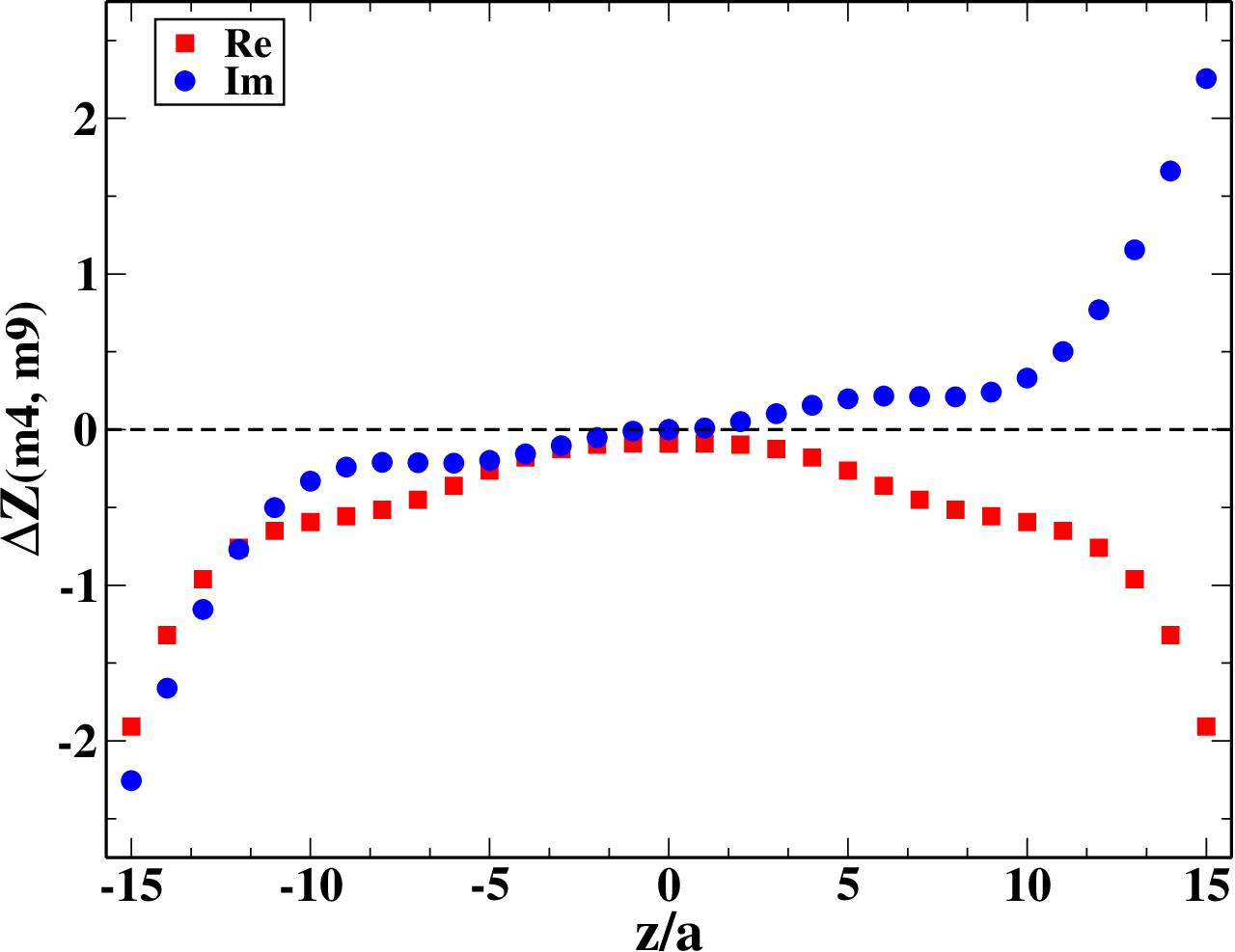
Based on the above, we conclude that the systematic uncertainties related to lattice artifacts and the conversion factor must be addressed, in order to extract reliable estimates on the renormalization functions. It is our intention to reduce both effects in the near future, which will eliminate systematic uncertainties propagated to the estimates of the quasi-PDFs. Understanding the uncertainties dominating the large- region is crucial, as the matrix element for these values also enters in the Fourier transform that yields the quasi-PDF. Preliminary explorations indicate that a likely magnitude of the two-loop contribution might suppress the imaginary part of . Even though we are currently in no position to accurately quantify these systematics, we will estimate upper bounds. In particular, we try to estimate the effect of each one individually.
Lattice artifacts
The -factor for the helicity quasi-PDF at reduces to the renormalization function of the local axial current . is scheme- and scale-independent, and thus, the case allows us to study the lattice artifacts. has been already evaluated for this ensemble in Ref. [38]. In the latter calculation several diagonal scales have been employed and, together with a technique for the removal of the lattice artifacts, the extracted value was found to be . In the present calculation at we find a value of using the scale m9 and for the scale m4. This is yet another indication that lattice artifacts are large for the “parallel” renormalization scale and less severe, but not negligible, for the “diagonal” case.
An additional test that may be performed for any value of is the comparison of between scales with different components, but same . For this, we utilize the values labeled as m10 and m11, which can be compared to m1 and m4, respectively. Since these pairs are approximately at the same value of , we can compare them directly in the RI′ scheme without any evolution44 4 We confirmed numerically that the conversion factors from m1 to m10, and from m4 to m11 deviates from unity by less than 1‰, so we ignore it., and the difference can be interpreted as lattice artifacts. We observe similar behavior for the two pairs and as a demonstration we plot in Fig. 7 the following ratio for each value of
| (18) |


In the left panel we show the case where and correspond to the values m4 and m11, respectively. The difference from zero can be attributed to lattice artifacts. We find that the -factor extracted from m11 deviates from the value extracted from m4 by 5-10% in the real part and up to 30% in the imaginary part. This deviation seems to stabilize after to 5% (10%) for the real (imaginary) part.
Note that the left plot of Fig. 7 gives the estimate of the discretization effects for the “parallel” case compared to the “diagonal” one. It would be interesting to compute between two neighboring “diagonal” momenta in order to understand the change in the artifacts. We choose 2 pairs (m2,m3) and (m5,m6) and we find that both and are less than 1%, while and are of the order of 6%. This is a confirmation that excluding “parallel” momenta in the fit of Eq. (17) reduces significantly the discretization effects.
Truncation effects
In order to assess quantitatively the influence of the conversion factor that is known to one-loop perturbation theory, we form the ratios
| (19) |
both for the real and imaginary parts of the helicity -factor. In Fig. 8, we plot Eq. (19) for the RI’ and case. These have been extracted at different values of (m1m8) and evolved perturbatively to the same scale of GeV, using the results of Ref. [25]. The ratio is always taken with respect to the smallest “diagonal” scale, m1. depend on the truncation effects in the one-loop evolution to 2 GeV, while is affected by scheme conversion truncation effects. Without contamination from lattice artifacts and truncation effects, Eq. (19) should equal 1 in both schemes and for all values of and . This realization allows for investigation of the truncation effects.


One observes that the imaginary part is more sensitive to the change of the initial RI′ scale, which is given in the x-axis. To demonstrate this, we keep the range of y-axis the same for all plots of Fig. 8. The difference between the ratios of the real part extracted from different RI′ scales is consistently small and reaches at most approx. 5% in the RI′ scheme and 3% in the scheme, regardless of the Wilson line length, . As we mentioned above, for we can compare to the highly reliable value found in Ref. [38]; our current value from the scale m1 is around 2% higher. Hence, we can estimate the typical size of discretization effects to be of order 2-5% in the real part of the -factors.
The differences in the ratios are combinations of lattice artifacts and the conversion truncation. We observe that the conversion to the scheme decreases the differences in the scheme to at most 3%. Hence, truncation alone in the real part seems not to have an effect larger than 2%. Since we know that conversion truncation effects are very small for small values of (in particular, they are zero for , where is scheme-independent), we can take 0-2% as our estimate. In the end, given the fact that truncation effects seem to be opposite to the influence of lattice artifacts, we estimate that the total effects present in the real part of should not exceed 5%.
The situation is somewhat different in the ratio of the imaginary parts shown in the right panel of Fig. 8. We conclude that the uncertainty from lattice artifacts can be of the order of 10% in the RI′ scheme for intermediate and large ( 55 5 For smaller values of , the imaginary part is small in absolute terms and Eq. (19) becomes meaningless, i.e. even small absolute changes of the imaginary part of can imply large changes in .). From the right panel of Fig. 8, the total uncertainty in can get enhanced to around 40% for large and up to 80% for intermediate Wilson line lengths. In addition, the total uncertainty in the imaginary part of is basically of the order of its magnitude, as it is expected to be real. Note that ignoring the imaginary part does not provide any solution, as they need to come out zero from the computation in order to claim that the computation is fully reliable. Thus, conversion truncation effects become the most major source of uncertainty of the imaginary parts of the -factors.
Based on the study presented in this subsection, we present in Table 2 a summary of our quantitative estimates on the systematic uncertainties present in . The estimate of the total effect is not a simple sum of isolated effects, but takes into account their different signs discussed above. For the imaginary part, the estimates are for , since for smaller values of and the relative effects become meaningless.
We would like to stress that due to the complex multiplication of the -factors and the bare matrix elements, the large uncertainty in the imaginary part of the -factor implies that also real part of the renormalized matrix elements is affected. Furthermore, the uncertainties that we consider in the -factors translate differently to the uncertainties of the renormalized matrix elements for different Wilson line lengths and thus, we postpone the discussion of this influence to the next subsection.
| Effect | ||
|---|---|---|
| Lattice artifacts | 2-5% | % |
| Evolution truncation | 1-2% | 1-2% |
| Conversion truncation | % | % |
| Total | 3-5% | % |
3.3 Renormalized results
Once the -factors are obtained for the unpolarized, helicity and transversity quasi-PDFs, one may proceed with the application of the renormalization in the nucleon matrix elements. Here we mostly focus on the helicity case, as the renormalization is multiplicative. The case of the unpolarized quasi-PDF is briefly mentioned in the end of the subsection.
In Fig. 9, we show the renormalized helicity nucleon matrix elements, and compare them with the bare ones. This is a straightforward procedure as there is no mixing for the axial operator and, therefore, the renormalization is only multiplicative:
| (20) |
The above formula involves complex quantities, and thus, is a mixture of the real and imaginary part of the bare matrix element. However, each value of is renormalized independently. We use from the extrapolation of Eq. (17) in the range , as shown in Fig. 4. One can see in Fig. 9 that for small values of there is a slight suppression of the renormalized real part with respect to the bare one (). is compatible with zero for , but with increased statistical uncertainties. The effect of the renormalization on the imaginary part of the matrix element is profound in the large region, where we observe an amplification of its value and a shift of the maximum to larger z, as compared to the bare one.


The renormalized matrix elements of the helicity quasi-PDF are presented here for the first time, and they demonstrate the enormous progress in the field of the quasi-PDFs. However, before attempting to compare with the physical PDFs, we must understand the uncertainties that are inherited to from its renormalization function. As we argued in the previous subsection, a robust computation needs the subtraction of lattice artifacts and a significant reduction of truncation uncertainties in the conversion between the RI′ and schemes. We attempt setting bounds on these systematics, starting with the real part of renormalized matrix elements, which reads:
| (21) |
For small values of , is approximately zero and thus is approximately equal to the first term of Eq. (21). On the contrary, for , receives significant contributions from the imaginary part, because .
The uncertainty in the small- region of renormalized matrix elements is dominated by uncertainties in the real part of the -factor, which, as argued in the previous subsection, should not exceed 5%. The local minimum observed at is likely to result from lattice artifacts and truncation effects. In the large- region, the real part of the renormalized matrix elements receives negative contributions from the imaginary part of the bare matrix element if has a non-zero imaginary part and decays to zero more slowly than , which is what we observe in the data. This effect is unphysical and is expected to be strongly suppressed or eliminated by extending our calculation to the two-loop order in the conversion and by subtracting lattice artifacts.
The imaginary part of renormalized matrix elements,
| (22) |
is enhanced in the intermediate- regime, compared to the bare matrix elements. This results mostly from the fact that increases with increasing at a faster rate, than the decay of . However, the obtained values receive also contributions from the second term of Eq. (22), where is subject to a large uncertainty, as discussed in the previous subsection.
We want to stress that it is not possible to give a single number for the relative uncertainty of the real and imaginary parts of . According to Eqs. (21) - (22), different regions of are influenced in a different way by the real and imaginary parts of the -factors. For small , where is small, the propagated uncertainty in the matrix elements is dominated by the uncertainty of , which is of the order of 5% and comparable to the currently attained statistical uncertainty. Thus, is rather robust in this region. However, when is increased, the uncertainty from starts to dominate and reaches 100% for large . In this way, the improvements expected by the perturbative subtraction of lattice artifacts and the extension to the two-loop perturbative conversion to the scheme are very important for obtaining meaningful values of renormalized matrix elements and hence, also quasi-PDFs.
The values of the multiplicative vector renormalization factor and the mixing coefficient can be used to properly renormalize the unpolarized quasi-PDF through Eq. (12). The successful renormalization requires the bare nucleon matrix elements for the scalar and vector operators, in order to extract the renormalized . Then, it must be multiplied by the conversion factor to bring the results to the scheme. Note that once the mixing is treated, the conversion factor is multiplicative and not a matrix. This is due to the fact that no mixing is present in the continuum dimensional regularization.
3.4 Matching to light-front PDFs
Having the renormalized matrix elements, one can perform a Fourier transform and obtain the renormalized quasi-PDF, which represents the distribution of quark momenta for a finite-momentum nucleon moving in the chosen spatial () direction:
| (23) |
where is the quark momentum fraction. The quasi-PDF, expressed in our case in the scheme at GeV, can then be connected to the light-front PDF, in the same scheme and at the same scale, using one-loop perturbative matching. The matching procedure uses the fact that only the ultraviolet physics is different in quasi- () and light-front () PDFs [11]. Hence, the one-loop difference between them is expressed as the difference between vertex corrections (denoted below) and wave function corrections () for the finite momentum and infinite momentum cases. The generic matching formula for quasi-PDFs is: [50, 12]
| (24) | |||||
where is the strong coupling constant at the scale . In the integral, we exclude a small region around , such that the argument of is not too large, as we would then pick up contributions from the mirror images of resulting from the periodicity of the Fourier transform in Eq. (23). The linearly divergent terms (: transverse momentum cutoff) of the matching formulae from Ref. [11] are not present in our renormalized results.

In Fig. 10, we show the matched helicity PDF computed with either fully renormalized matrix elements obtained in this work (blue) or with bare matrix elements multiplied by the local () axial vector current renormalization function (magenta), corresponding to our results from Ref. [17]. We observe that the renormalized matrix elements from this work move towards the phenomenological PDFs, which is promising. In particular, the antiquark asymmetry is not overestimated any longer and actually this asymmetry becomes compatible with zero under current uncertainties. In the quark part, there is an enhancement of the matched PDF for all values of . We emphasize again that the comparison with the phenomenological PDFs should be understood as only qualitative. For quantitative comparison, a careful investigation of a number of systematic effects is still needed. These include: cut-off effects, non-physical pion mass, finite volume effects, possible contamination by excited states, extrapolation to infinite nucleon boost, as well as the improvements in the computation of renormalization functions, postulated in the previous subsection: subtraction of lattice artifacts computed in lattice perturbation theory and reduction of truncation effects in the perturbative conversion to the scheme.
4 Conclusions and discussion
In this work we have presented a concrete prescription to renormalize non-perturbatively the matrix elements needed for the computation of quasi-PDFs. The employed scheme is RI′, which is then converted to the scheme and evolved to 2 GeV; this is done perturbatively to one-loop. We have argued that the renormalization condition properly handles both kinds of divergences present in the matrix elements: the standard logarithmic divergence and the power divergence specific to non-local operators containing a Wilson line. Furthermore, we provide the renormalization conditions to eliminate the mixing in the case of the unpolarized quasi-PDF that mixes with the twist-3 scalar operator.
We have also demonstrated the implementation of the proposed prescription to the helicity quasi-PDF and presented the corresponding renormalized matrix elements. This has allowed us to draw conclusions how to make the computation more robust, which is the main outcome of this work.
- •
First, an essential ingredient of a computation with controlled systematic uncertainties is the subtraction of one-loop lattice artifacts in the framework of lattice perturbation theory. Following the ideas of Ref. [38], we are currently computing the artifacts that will be subtracted from the non-perturbative estimates for the -factors. In this way, the presence of large cut-off effects in the renormalized functions (especially for “parallel” momenta) will be avoided to a large extent.
- •
Second, the conversion factor from the RI′ renormalization scheme to the scheme is likely to have sizable higher order corrections that, among others, are responsible for the unphysical feature of the real part of the renormalized matrix element becoming negative for large Wilson line lengths. A two-loop computation of this conversion factor is expected to resolve this issue to a sufficient degree. We have performed numerical experiments that indicate that a natural change of the conversion factor by two-loop contributions, i.e. around 10-20% (which is approximately at the considered scale), should be enough to suppress the unwanted effect. A perturbative calculation of the conversion factor to two loops is quite laborious and will be presented separately.
To summarize, the renormalization program presented in this work together with future improvements that are being pursued, will provide reliable estimates for the renormalization functions of the Wilson line fermion operators. In this fashion, the obtained renormalized matrix elements can be used as an input to calculate the quasi-PDFs and match them to light-front PDFs, which is the main aim of the whole approach. Apart from the helicity case discussed in this work, we will address the transversity PDF in an analogous manner. For the unpolarized case, one needs to take into account the mixing with the scalar operator, as explained and numerically demonstrated here. With this work, we have proposed and discussed a complete renormalization program of the quasi-PDFs, which has been a major uncertainty prior to this work and constitutes a crucial milestone in connecting lattice QCD results to the light-cone PDFs.
Acknowledgements
We would like to thank the members of ETMC for useful and fruitful discussions. We also thank Rainer Sommer for discussions related to the arbitrary scale in the renormalization prescription. An award of computer time was provided by the INCITE program. This research also used resources of the Oak Ridge Leadership Computing Facility, which is a DOE Office of Science User Facility supported under Contract DE-AC05-00OR22725. KC was supported in part by the Deutsche Forschungsgemeinschaft (DFG), project nr. CI 236/1-1. MC acknowledges financial support by the U.S. Department of Energy, Office of Science, Office of Nuclear Physics, within the framework of the TMD Topical Collaboration, as well as, by the National Science Foundation under Grant No. PHY-1714407. We acknowledge funding from the European Union’s Horizon 2020 research and innovation program under the Marie Sklodowska-Curie grant agreement No 642069.
References
- [1] R. P. Feynman, Photon-Hadron Interactions, Frontiers in Physics, Benjamin, Reading, MA, 1972.
- [2] M. Constantinou, Hadron Structure, PoS LATTICE2014 (2014) 001. arXiv:1411.0078.
- [3] M. Constantinou, Recent progress in hadron structure from Lattice QCD, PoS CD15 (2015) 009. arXiv:1511.00214.
- [4] C. Alexandrou, K. Jansen, Hadron structure from lattice QCD, Nucl. Part. Phys. Proc. 261-262 (2015) 202.
- [5] C. Alexandrou, Selected results on hadron structure using state-of-the-art lattice qcd simulations, in: Proceedings, 45th International Symposium on Multiparticle Dynamics (ISMD 2015): Kreuth, Germany, October 4-9, 2015, 2015. arXiv:1512.03924.
- [6] S. Syritsyn, Review of Hadron Structure Calculations on a Lattice, PoS LATTICE2013 (2014) 009. arXiv:1403.4686.
- [7] P. Jimenez-Delgado, W. Melnitchouk, J. F. Owens, Parton momentum and helicity distributions in the nucleon, J. Phys. G40 (2013) 093102. arXiv:1306.6515.
- [8] A. Accardi, L. T. Brady, W. Melnitchouk, J. F. Owens, N. Sato, Constraints on large- parton distributions from new weak boson production and deep-inelastic scattering data, Phys. Rev. D93 (2016) 114017. arXiv:1602.03154.
- [9] S. Alekhin, J. Blumlein, S. Moch, R. Placakyte, Parton distribution functions, , and heavy-quark masses for LHC Run II, Phys. Rev. D96 (2017) 014011. arXiv:1701.05838.
- [10] X. Ji, Parton Physics on a Euclidean Lattice, Phys. Rev. Lett. 110 (2013) 262002. arXiv:1306.1539.
- [11] X. Xiong, X. Ji, J.-H. Zhang, Y. Zhao, One-loop matching for parton distributions: Nonsinglet case, Phys. Rev. D90 (2014) 014051. arXiv:1310.7471.
- [12] J.-W. Chen, X. Ji, J.-H. Zhang, Improved quasi parton distribution through Wilson line renormalization, Nucl. Phys. B915 (2017) 1. arXiv:1609.08102.
- [13] H.-W. Lin, J.-W. Chen, S. D. Cohen, X. Ji, Flavor Structure of the Nucleon Sea from Lattice QCD, Phys. Rev. D91 (2015) 054510. arXiv:1402.1462.
- [14] L. Gamberg, Z.-B. Kang, I. Vitev, H. Xing, Quasi-parton distribution functions: a study in the diquark spectator model, Phys. Lett. B743 (2015) 112. arXiv:1412.3401.
- [15] C. Alexandrou, K. Cichy, V. Drach, E. Garcia-Ramos, K. Hadjiyiannakou, K. Jansen, F. Steffens, C. Wiese, Lattice calculation of parton distributions, Phys. Rev. D92 (2015) 014502. arXiv:1504.07455.
- [16] J.-W. Chen, S. D. Cohen, X. Ji, H.-W. Lin, J.-H. Zhang, Nucleon Helicity and Transversity Parton Distributions from Lattice QCD, Nucl. Phys. B911 (2016) 246. arXiv:1603.06664.
- [17] C. Alexandrou, K. Cichy, M. Constantinou, K. Hadjiyiannakou, K. Jansen, F. Steffens, C. Wiese, Updated Lattice Results for Parton Distributions, Phys. Rev. D96 (2017) 014513. arXiv:1610.03689.
- [18] A. Radyushkin, Target Mass Effects in Parton Quasi-Distributions, Phys. Lett. B770 (2017) 514. arXiv:1702.01726.
- [19] A. Radyushkin, Nonperturbative Evolution of Parton Quasi-Distributions, Phys. Lett. B767 (2017) 314. arXiv:1612.05170.
- [20] A. V. Radyushkin, Quasi-parton distribution functions, momentum distributions, and pseudo-parton distribution functions, Phys. Rev. D96 (2017) 034025. arXiv:1705.01488.
- [21] K. Orginos, A. Radyushkin, J. Karpie, S. Zafeiropoulos, Lattice QCD exploration of pseudo-PDFs, arXiv:1706.05373.
- [22] C. E. Carlson, M. Freid, Lattice corrections to the quark quasidistribution at one-loop, Phys. Rev. D95 (2017) 094504. arXiv:1702.05775.
- [23] R. A. Briceño, M. T. Hansen, C. J. Monahan, Role of the Euclidean signature in lattice calculations of quasidistributions and other nonlocal matrix elements, Phys. Rev. D96 (2017) 014502. arXiv:1703.06072.
- [24] V. S. Dotsenko, S. N. Vergeles, Renormalizability of Phase Factors in the Nonabelian Gauge Theory, Nucl. Phys. B169 (1980) 527.
- [25] M. Constantinou, H. Panagopoulos, Perturbative Renormalization of quasi-PDFs, Phys. Rev. D 96 (2017) 054506. arXiv:1705.11193.
- [26] Y.-Q. Ma, J.-W. Qiu, Extracting Parton Distribution Functions from Lattice QCD Calculations, arXiv:1404.6860.
- [27] T. Ishikawa, Y.-Q. Ma, J.-W. Qiu, S. Yoshida, Practical quasi parton distribution functions, arXiv:1609.02018.
- [28] C. Monahan, K. Orginos, Quasi parton distributions and the gradient flow, JHEP 03 (2017) 116. arXiv:1612.01584.
- [29] X. Ji, J.-H. Zhang, Y. Zhao, Renormalization in Large Momentum Effective Theory of Parton Physics, arXiv:1706.08962.
- [30] J. Green, K. Jansen, F. Steffens, Nonperturbative renormalization of nonlocal quark bilinears for quasi-PDFs on the lattice using an auxiliary field, arXiv:1707.07152.
- [31] T. Ishikawa, Y.-Q. Ma, J.-W. Qiu, S. Yoshida, On the Renormalizability of Quasi Parton Distribution Functions, arXiv:1707.03107.
- [32] J.-W. Chen, T. Ishikawa, L. Jin, H.-W. Lin, Y.-B. Yang, J.-H. Zhang, Y. Zhao, Parton Distribution Function with Non-perturbative Renormalization from Lattice QCD, arXiv:1706.01295.
- [33] G. Martinelli, C. Pittori, C. T. Sachrajda, M. Testa, A. Vladikas, A General method for nonperturbative renormalization of lattice operators, Nucl. Phys. B445 (1995) 81. arXiv:hep-lat/9411010.
- [34] R. Baron, P. Boucaud, J. Carbonell, A. Deuzeman, V. Drach, et al., Light hadrons from lattice QCD with light (u,d), strange and charm dynamical quarks, JHEP 1006 (2010) 111. arXiv:1004.5284.
- [35] N. Carrasco, et al., Up, down, strange and charm quark masses with Nf = 2+1+1 twisted mass lattice QCD, Nucl. Phys. B887 (2014) 19. arXiv:1403.4504.
- [36] R. Sommer, Non-perturbative Heavy Quark Effective Theory: Introduction and Status, Nucl. Part. Phys. Proc. 261-262 (2015) 338. arXiv:1501.03060.
- [37] C. Alexandrou, M. Constantinou, T. Korzec, H. Panagopoulos, F. Stylianou, Renormalization constants for 2-twist operators in twisted mass QCD, Phys. Rev. D83 (2011) 014503. arXiv:1006.1920.
- [38] C. Alexandrou, M. Constantinou, H. Panagopoulos, Renormalization functions for Nf=2 and Nf=4 twisted mass fermions, Phys. Rev. D95 (2017) 034505. arXiv:1509.00213.
- [39] M. Constantinou, et al., Non-perturbative renormalization of quark bilinear operators with Nf = 2 (tmQCD) Wilson fermions and the tree-level improved gauge action, JHEP 08 (2010) 068. arXiv:1004.1115.
- [40] A. Abdel-Rehim, et al., Simulating QCD at the Physical Point with Wilson Twisted Mass Fermions at Maximal Twist, , Phys. Rev. D95 (2017) 094515. arXiv:1507.05068.
- [41] A. Abdel-Rehim, et al., Nucleon and pion structure with lattice QCD simulations at physical value of the pion mass, Phys. Rev. D92 (2015) 114513. arXiv:1507.04936.
- [42] M. Constantinou, R. Horsley, H. Panagopoulos, H. Perlt, P. E. L. Rakow, G. Schierholz, A. Schiller, J. M. Zanotti, Renormalization of local quark-bilinear operators for =3 flavors of stout link nonperturbative clover fermions, Phys. Rev. D91 (2015) 014502. arXiv:1408.6047.
- [43] A. J. Buras, P. H. Weisz, QCD Nonleading Corrections to Weak Decays in Dimensional Regularization and ’t Hooft-Veltman Schemes, Nucl. Phys. B333 (1990) 66.
- [44] A. Patel, S. R. Sharpe, Perturbative corrections for staggered fermion bilinears, Nucl. Phys. B395 (1993) 701. arXiv:hep-lat/9210039.
- [45] S. A. Larin, J. A. M. Vermaseren, The Three loop QCD Beta function and anomalous dimensions, Phys. Lett. B303 (1993) 334. arXiv:hep-ph/9302208.
- [46] S. A. Larin, The Renormalization of the axial anomaly in dimensional regularization, Phys. Lett. B303 (1993 [See also hep-ph/9302240 for an additional Section]) 113. arXiv:hep-ph/9302240.
- [47] A. Skouroupathis, H. Panagopoulos, Two-loop renormalization of vector, axial-vector and tensor fermion bilinears on the lattice, Phys. Rev. D79 (2009) 094508. arXiv:0811.4264.
- [48] M. Constantinou, M. Costa, H. Panagopoulos, Perturbative renormalization functions of local operators for staggered fermions with stout improvement, Phys. Rev. D88 (2013) 034504. arXiv:1305.1870.
- [49] M. Gockeler, R. Horsley, H. Oelrich, H. Perlt, D. Petters, P. E. L. Rakow, A. Schafer, G. Schierholz, A. Schiller, Nonperturbative renormalization of composite operators in lattice QCD, Nucl. Phys. B544 (1999) 699. arXiv:hep-lat/9807044.
- [50] X. Ji, J.-H. Zhang, Renormalization of quasiparton distribution, Phys. Rev. D92 (2015) 034006. arXiv:1505.07699.
- [51] D. de Florian, R. Sassot, M. Stratmann, W. Vogelsang, Extraction of Spin-Dependent Parton Densities and Their Uncertainties, Phys. Rev. D80 (2009) 034030. arXiv:0904.3821.
- [52] N. Sato, W. Melnitchouk, S. E. Kuhn, J. J. Ethier, A. Accardi, Iterative Monte Carlo analysis of spin-dependent parton distributions, Phys. Rev. D93 (2016) 074005. arXiv:1601.07782.