跳到论文正文
W Papers独立论文阅读器 arXiv:1706.00223 论文正文 计算阅读时间 · 0%
引用这篇论文根据当前论文元数据生成,正式投稿前建议核对。


License: arXiv.org perpetual non-exclusive license
arXiv:1706.00223v1 [physics.flu-dyn] 01 Jun 2017

NONLINEAR VORTEX STRUCTURES IN OBLIQUELY ROTATING STRATIFIED FLUIDS DRIVEN BY SMALL SCALE NON HELICAL FORCES

Affiliation: M.I. Kopp Affiliation: A.V. Tur Affiliation: V.V. Yanovsky
Abstract

In this paper, we study a new type of large-scale instability in obliquely rotating stratified fluids with small scale non-helical turbulence. The small-scale turbulence is generated by the external force with zero helicity and low Reynolds number. The theory uses the method of multiscale asymptotic developments. The nonlinear equations for large scale motions are obtained in the third order of the perturbation theory. In this paper, we consider the linear instability and the stationary nonlinear modes. We obtain solutions in the form of nonlinear Beltrami waves and localized vortex structures as kinks of new type.

1 Institute for Single Crystals, NAS Ukraine, Nauky Ave. 60, Kharkov 61001, Ukraine

2 V.N. Karazin Kharkiv National University 4 Svobody Sq., Kharkov 61022, Ukraine

3Université de Toulouse [UPS], CNRS, Institut de Recherche en Astrophysique
et Planétologie, 9 avenue du Colonel Roche, BP 44346, 31028 Toulouse Cedex 4, France

1 Introduction

The problem of generation of large-scale vortex motions and formation of stationary nonlinear vortex structures in turbulent media is very important. The characteristic scales of the velocity fields for these structures are much bigger than the characteristic scales of turbulent motions or waves which engender their appearance. The study of the generation mechanism of large-scale vortex structures (LSVS) by small-scale turbulence has not only scientific but also application interest. For instance, tornados, cyclones and anticyclones represent the particular cases of LSVS. They also play an important role in the dynamics of Earth’s atmosphere, since they determine the global transport of air masses and are responsible for the weather and climate on our planet [1]-[3]. The study of the mechanisms of LSVS generation is important for a number of astrophysical problems, such as the origin of the Great Spot of Jupiter, Venus super rotation, vortex structures in solar prominences and so on [4]-[8]. The generation of LSVS in atmospheres and bowels of the planets (or other space objects) is essentially due to thermal phenomena occurring under the influence of internal or external sources of the thermal energy. Articles [9]-[11] present the theory of convective vortex dynamo. It follows from this theory that the small-scale helical turbulence leads to a large-scale instability, which engenders the formation of one convective cell considered as a huge vortex of type of tropical cyclone. Number of numerical [12] and laboratory [13] experiments confirm this. The theory of the convective vortex dynamo was further developed in [14], [15], applying the method of multiscale asymptotic developments. This method, unlike the functional techniques [16], [17] used in [9]-[11] allows to determine strictly the principal order of perturbations theory in which the instability arises. The method of multiscale asymptotic developments to describe the generation of LSVS in reflective non invariant turbulence was first used in [18]. The small Reynolds number is a parameter of the asymptotic developments. Nonlinear stabilization of the convective large-scale instability discussed in [14],[15] leads to the formation of helical vortex solitons or kinks of a new type. The generation of helical turbulence in natural conditions is usually associated with the influence of the Coriolis force on turbulent motion [19], [20]. Obviously, the question arises of the possibility of generation of large-scale vortex field in a rotating media under influence of small-scale force with zero helicity. An example of the generation of LSVS in a rotating incompressible fluid was found in [21]. It was also shown that the development of large-scale instability in an inclined rotating fluid generates the nonlinear large-scale helical vortex structures or localized Beltrami vortices with the internal helical structure.

In this paper we give a generalization of the α\alpha – effect found in [21] for the case of temperature- stratified fluid. As a result of this generalization, we obtain the large-scale instability which generates the LSVS.

The organization of this paper is as follows. In the Section 2 we obtain the averaged hydrodynamic equations in the Boussinesq approximation in an obliquely rotating fluid for the large-scale fields using the method of multiscale asymptotic developments. The technical aspect of this question is described in detail in Appendix I. The correlation functions in the averaged equations are expressed in terms of the small-scale fields in the zero-order approximation with respect to RR. In Appendix II in order to obtain the averaged equations in closed form, we find solutions for small-scale fields of zero order approximation. In Appendix III we calculate the Reynolds stresses using these solutions. In Sec. 2 we obtain a closed system of the nonlinear equations for large-scale vortex fields (vortex dynamo). In Section 3 we consider the generation of small large-scale vortex perturbations, which arises from instability of the type α\alpha – effect. Also the conditions of the appearance of this instability are determined depending on the effects of rotation and stratification of the medium. In Section 4, an analytic and numerical analysis of nonlinear equations in the steady state is performed, which shows the existence of nonlinear Beltrami waves and localized vortex structures in the form of kinks. The results obtained in the work can be applied to the numerous geophysical and astrophysical problems.

2 Equations for the large-scale fields

Let us consider a system of equations for the perturbations of velocity v→\vec{v}, temperature TT, pressure PP in the Boussinesq approximation with the constant temperature gradient ∇T¯\nabla\overline{T} for a rotating coordinate system:

∂vi∂t+vk​∂vi∂xk=ν​Δ​vi−1ρ¯​∂P∂xi+2​εi​j​k​vj​Ωk+g​ei​β​T+F0i\frac{\partial v_{i}}{\partial t}+v_{k}\frac{\partial v_{i}}{\partial x_{k}}=\nu\Delta v_{i}-\frac{1}{\overline{\rho}}\frac{\partial P}{\partial x_{i}}+2\varepsilon_{ijk}v_{j}{\Omega}_{k}+ge_{i}\beta T+F_{0}^{i} (1)
∂T∂t+vk​∂T∂xk−A​ek​vk=χ​Δ​T\frac{\partial T}{\partial t}+v_{k}\frac{\partial T}{\partial x_{k}}-Ae_{k}v_{k}=\chi\Delta T (2)
∂vi∂xi=0\frac{\partial v_{i}}{\partial x_{i}}=0 (3)

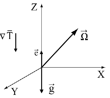
The system of equations (1)-(3) describes the evolution of perturbations on the background of the basic equilibrium state T¯​(z)\overline{T}\left(z\right), ρ¯​(z)\overline{\rho}\left(z\right), which is set by the constant temperature gradient ∇T¯=−A​e→​(A>0)\nabla\overline{T}=-A\vec{e}(A>0) (heated from below) and by the hydrostatic pressure: ∇P¯=ρ¯​g→−ρ¯​[Ω→×[Ω→×r→]]\nabla\overline{P}=\overline{\rho}\vec{g}-\overline{\rho}\left[\vec{\Omega}\times\left[\vec{\Omega}\times\vec{r}\right]\right], where r→\vec{r} is the radius-vector of the fluid element. We consider the angular velocity of rotation Ω→\vec{\Omega} as constant (solid rotation) and inclined to the plane (X,Y)(X,Y), as shown in Fig. 1, i.e. for the Cartesian geometry problem: Ω→=(Ω1,Ω2,Ω3)\vec{\Omega}=\left(\Omega_{1},\Omega_{2},\Omega_{3}\right) . Where e→=(0,0,1)\vec{e}=(0,0,1) is unit vector in the direction of the axis ZZ, g→\vec{g} is the gravity directed vertically downwards g→=(0,0,−g)\vec{g}=(0,0,-g), β\beta is the coefficient of thermal expansion. The equation (1) includes the external force F→0\vec{F}_{0}, that models the excitation source in the environment of small scale and high frequency fluctuations of the velocity field with small Reynolds number. Unlike the previous studies [14], [15] we consider here the non-helical external force with the following properties:

d​i​v​F→0=0,F→0​r​o​t​F→0=0,r​o​t​F→0≠0,F→0=f0​F→0​(xλ0,tt0)div\vec{F}_{0}=0,\;\vec{F}_{0}rot\vec{F}_{0}=0,\;rot\vec{F}_{0}\neq 0,\;\vec{F}_{0}=f_{0}\vec{F}_{0}\left(\frac{x}{\lambda_{0}};\frac{t}{t_{0}}\right) (4)

Where λ0\lambda_{0} is the characteristic scale, t0t_{0} is the characteristic time, f0f_{0} is the characteristic amplitude. The external force is given in the plane (X,Y)(X,Y) , where the perpendicular projection of the angular velocity is located. We choose the external force in rotating coordinate system in the following form :

F0z=0,F→0⊥=f0​(i→​c​o​s​ϕ2+j→​c​o​s​ϕ1),ϕ1=k→1​x→−ω0​t,ϕ2=k→2​x→−ω0​t,F_{0}^{z}=0,\;\vec{F}_{0\bot}=f_{0}\left(\vec{i}cos\phi_{2}+\vec{j}cos\phi_{1}\right),\;\phi_{1}=\vec{k}_{1}\vec{x}-\omega_{0}t,\phi_{2}=\vec{k}_{2}\vec{x}-\omega_{0}t,
k→1=k0​(1,0,0),k→2=k0​(0,1,0).\vec{k}_{1}=k_{0}\left(1,0,0\right),\vec{k}_{2}=k_{0}\left(0,1,0\right). (5)
Refer to caption
Figure 1: In general case, the angular velocity Ω→\vec{\Omega} is inclined to the plane (X,Y)(X,Y) where the external force F→0⊥\vec{F}_{0\bot} is located.

Obviously, this non-helical external force satisfies all the conditions (4). Let us now use in equations (1)-(3) the dimensionless variables. For convenience, we will designate these variables like dimensional variables:

x→→x→λ0,t→tt0,v→→v→v0,F→0→F→0f0,P→Pρ¯​p0,\vec{x}\to\frac{\vec{x}}{\lambda_{0}},\quad t\to\frac{t}{t_{0}},\quad\vec{v}\to\frac{\vec{v}}{v_{0}},\quad\vec{F}_{0}\to\frac{\vec{F}_{0}}{f_{0}},\quad P\to\frac{P}{\overline{\rho}p_{0}},
t0=λ02ν,p0=v0​νλ0,f0=v0​νλ02,T→Tλ0​At_{0}=\frac{\lambda_{0}^{2}}{\nu},\quad p_{0}=\frac{v_{0}\nu}{\lambda_{0}},\quad f_{0}=\frac{v_{0}\nu}{\lambda_{0}^{2}},\quad T\to\frac{T}{\lambda_{0}A} (6)

Then, in dimensionless variables the equation (1)-(3) takes the following form:

∂vi∂t+R​vk​∂vi∂xk=Δ​vi−∂P∂xi+εi​j​k​vj​Dk+ei​R​a~​T+F0i\frac{\partial v_{i}}{\partial t}+Rv_{k}\frac{\partial v_{i}}{\partial x_{k}}=\Delta v_{i}-\frac{\partial P}{\partial x_{i}}+\varepsilon_{ijk}v_{j}D_{k}+e_{i}\widetilde{Ra}T+F_{0}^{i} (7)
∂T∂t+R​vk​∂T∂xk−ek​vk=P​r−1​Δ​T\frac{\partial T}{\partial t}+Rv_{k}\frac{\partial T}{\partial x_{k}}-e_{k}v_{k}=Pr^{-1}\Delta T (8)
∂vi∂xi=0\frac{\partial v_{i}}{\partial x_{i}}=0 (9)

Here, R​a~=R​aP​r\widetilde{Ra}=\frac{Ra}{Pr}, R​a=g​β​A​λ04ν​χRa=\frac{g\beta A\lambda_{0}^{4}}{\nu\chi} is the Rayleigh number for the scale λ0\lambda_{0}, P​r=νχPr=\frac{\nu}{\chi} is the Prandtl number, Di=2​Ωi​λ02νD_{i}=\frac{2\Omega_{i}\lambda_{0}^{2}}{\nu} is the dimensionless parameter of rotation for the scale λ0\lambda_{0} related with the Taylor number T​ai=Di2Ta_{i}=D_{i}^{2} which is the characteristic of the influence of Coriolis force on viscous forces.

We will consider the Reynolds number R=v0​t0λ0≪1R=\frac{v_{0}t_{0}}{\lambda_{0}}\ll 1 on the scale λ0\lambda_{0} as a small parameter of an asymptotic development. Concerning the parameters DiD_{i} and R​aRa , we do not choose any range of values for the moment. Let us examine the following formulation of the problem. We consider the external force as small and of high frequency. This force leads to the small scale fluctuations in velocity and temperature fields on the equilibrium background. After averaging, these quickly oscillating fluctuations vanish. Nevertheless, due to the small nonlinear interactions in some orders of perturbation theory, nonzero terms can occur after averaging. This means that they are not oscillatory and are of large scale. From a formal point of view, these terms are secular, i.e., they create the conditions for the solvability of large scale asymptotic development. So the purpose of this paper is to find and study the solvability equations, i.e., the equations for large scale perturbations. The method of asymptotic equations is well presented in works [7], [14], [15]. In accordance with these papers we introduce spatial and temporal derivatives in equations (7)-(9) in the form of asymptotic expansions:

∂∂t→∂t+R4∂T,∂∂xi→∂i+R2∇i\frac{\partial}{\partial t}\to\partial_{t}+R^{4}\partial_{T},\;\;\;\frac{\partial}{\partial x_{i}}\to\partial_{i}+R^{2}\nabla_{i} (10)

where∂i\partial_{i} and ∂t\partial_{t} denote derivatives with respect to fast variables x0=(x→0,t0)x_{0}=\left(\vec{x}_{0},t_{0}\right) and ∇i\nabla_{i},∂T\partial_{T} derivatives with respect to slow variable X=(X→,T)X=\left(\vec{X},\;T\right) . Variables x0x_{0} and XX can be called small-scale and large-scale variables. To construct the nonlinear theory, the variables v→\vec{v}, T→\vec{T}, PP are presented in the form of asymptotic series:

v→​(x→,t)=1R​W→−1​(X)+v→0​(x0)+R​v→1+R2​v→2+R3​v→3+⋯\vec{v}(\vec{x},t)=\frac{1}{R}\vec{W}_{-1}\left(X\right)+\vec{v}_{0}\left(x_{0}\right)+R\vec{v}_{1}+R^{2}\vec{v}_{2}+R^{3}\vec{v}_{3}+\cdots
T⁡(x→,t)=1R​T−1​(X)+T0​(x0)+R​T1+R2​T2+R3​T3+⋯T(\vec{x},t)=\frac{1}{R}T_{-1}\left(X\right)+T_{0}\left(x_{0}\right)+RT_{1}+R^{2}T_{2}+R^{3}T_{3}+\cdots (11)
P⁡(x→,t)=1R3​P−3+1R2​P−2+1R​P−1+P0+R⁡(P1+P¯1​(X))+R2​P2+R3​P3+⋯P(\vec{x},t)=\frac{1}{R^{3}}P_{-3}+\frac{1}{R^{2}}P_{-2}+\frac{1}{R}P_{-1}+P_{0}+R(P_{1}+\overline{P}_{1}\left(X\right))+R^{2}P_{2}+R^{3}P_{3}+\cdots

Substituting developments (10)-(11) into the initial equations (7)-(9) and then gathering together the terms of the same order, we obtain the equations of the multi-scale asymptotic development and write down the obtained equations up to order R3R^{3} including. The algebraic structure of the asymptotic development of equations (7)-(9) in various orders of RR is given in Appendix I. It is also shown that in order R3R^{3} we get the main secular equation or equation for the large-scale fields:

∂TW−1i−Δ​W−1i+∇k(v0k​v0i¯)=−∇iP¯1\partial_{T}W_{-1}^{i}-\Delta W_{-1}^{i}+\nabla_{k}\left(\overline{v_{0}^{k}v_{0}^{i}}\right)=-\nabla_{i}\overline{P}_{1} (12)
∂TT−1−P​r−1​Δ​T−1=−∇k(v0k​T0¯)\partial_{T}T_{-1}-Pr^{-1}\Delta T_{-1}=-\nabla_{k}\left(\overline{v_{0}^{k}T_{0}}\right) (13)

Equations (12)-(13) with secular equations are obtained in Appendix I:

−∇iP−3+R​a~​ei​T−1+εi​j​k​Wj​Dk=0-\nabla_{i}P_{-3}+\widetilde{Ra}e_{i}T_{-1}+\varepsilon_{ijk}W_{j}D_{k}=0
Refer to caption
Figure 2: Relation of Cartesian projections of rotation parameter D→\vec{D} (or angular velocity of rotation Ω→\vec{\Omega}) with their projections in a spherical coordinate system.
W−1k​∇kW−1i=−∇iP−1W_{-1}^{k}\nabla_{k}W_{-1}^{i}=-\nabla_{i}P_{-1}
W−1k​∇kT−1=0W_{-1}^{k}\nabla_{k}T_{-1}=0
∇iW−1i=0\nabla_{i}W_{-1}^{i}=0
W−1z=0\ W_{-1}^{z}=0

These equations are satisfied by choosing the following geometry for the velocity field:

W→−1=(W−1x(Z),W−1y(Z),0),T−1=T−1(Z),P−1=const\vec{W}_{-1}=\left(W_{-1}^{x}\left(Z\right),\quad W_{-1}^{y}\left(Z\right),0\right),\quad T_{-1}=T_{-1}\left(Z\right),\quad P_{-1}=const (14)

In the frame of this quasi-two-dimensional approximation, we assume that the large-scale derivative over ZZ is much more than others derivatives, i.e.,

∇Z≡∂∂Z≫∂∂X,∂∂Y\nabla_{Z}\equiv\frac{\partial}{\partial Z}\gg\frac{\partial}{\partial X},\;\frac{\partial}{\partial Y}

Then the system of equations (12)-(13) is simplified and takes the following form:

∂TW1−∇Z2W1+∇Z(v0z​v0x¯)=0,W−1x=W1\partial_{T}W_{1}-\nabla_{{Z}}^{2}W_{1}+\nabla_{Z}\left(\overline{v_{0}^{z}v_{0}^{x}}\right)=0,\quad W_{-1}^{x}=W_{1} (15)
∂TW2−∇Z2W2+∇Z(v0z​v0y¯)=0,W−1y=W2\partial_{T}W_{2}-\nabla_{{Z}}^{2}W_{2}+\nabla_{Z}\left(\overline{v_{0}^{z}v_{0}^{y}}\right)=0,\quad W_{-1}^{y}=W_{2} (16)
∂TT−1−P​r−1​Δ​T−1+∇Z(v0z​T0¯)=0\partial_{T}T_{-1}-Pr^{-1}{\Delta T}_{-1}+\nabla_{{Z}}\left(\overline{{v}_{0}^{{z}}{T}_{0}}\right)=0 (17)

Equations (15)-(16) describe the evolution of large-scale eddy fields W→\vec{W} . In order to obtain the final closed form of equations (15)-(16) we have to calculate the Reynolds stresses ∇k(v0k​v0i¯)\nabla_{k}\left(\overline{v_{0}^{k}v_{0}^{i}}\right). This shows that we need to find solutions for the small-scale velocity field v→0\vec{v}_{0}. Appendix II contains a detailed technique to calculate the velocity field in a rotating stratified medium. Further, in Appendix III solutions for small-scale velocity field v→0\vec{v}_{0} are used to find the Reynolds stresses. Then equations (15)-(16) take a closed form:

(∂T−∇Z2)W~1=f022D2∇Z[1+W~22−R​a(1+W~22)​((1+W~22)2+2​(D22−R​a)​(1−W~22)+(D22−R​a)2)](\partial_{T}-\nabla_{Z}^{2})\widetilde{W}_{1}=\frac{{f_{0}^{2}}}{2}D_{2}\nabla_{Z}\left[{\frac{{1+\widetilde{W}_{2}^{2}-Ra}}{{(1+\widetilde{W}_{2}^{2})((1+\widetilde{W}_{2}^{2})^{2}+2(D_{2}^{2}-Ra)(1-\widetilde{W}_{2}^{2})+(D_{2}^{2}-Ra)^{2})}}}\right] (18)
(∂T−∇Z2)W~2=−f022D1∇Z[1+W~12−R​a(1+W~12)​((1+W~12)2+2​(D12−R​a)​(1−W~12)+(D12−R​a)2)](\partial_{T}-\nabla_{Z}^{2})\widetilde{W}_{2}=-\frac{{f_{0}^{2}}}{2}D_{1}\nabla_{Z}\left[{\frac{{1+\widetilde{W}_{1}^{2}-Ra}}{{(1+\widetilde{W}_{1}^{2})((1+\widetilde{W}_{1}^{2})^{2}+2(D_{1}^{2}-Ra)(1-\widetilde{W}_{1}^{2})+(D_{1}^{2}-Ra)^{2})}}}\right] (19)

To simplify the equations, we use here the designations: W~1=1−W1\widetilde{W}_{1}=1-W_{1} , W~2=1−W2\widetilde{W}_{2}=1-W_{2}. Thus, in this section we obtain the closed equations (18)-(19), which will be called the equations of nonlinear vortex dynamo in obliquely rotating stratified fluids with small scale non-helical force. If the rotation effect disappears (Ω=0\Omega=0 ), then the usual diffusion dissipation of large-scale fields occurs. In the limit of a homogeneous fluid the equation (18), (19) coincide with the results of [21]. We consider first the stability of small perturbations of fields (linear theory) and then examine the question of the possible existence of stationary structures.

3 Large-scale instability

Equations (18)-(19) describe the nonlinear dynamics of large scale disturbances of the vortex field W→=(W1,W2)\vec{W}=\left(W_{1},W_{2}\right). Therefore it is interesting to clarify the question of the stability of small perturbations of the field W→\vec{W}. Then for small values (W1,W2)\left(W_{1},W_{2}\right) the equations (18)-(19) are linearized and can be reduced to the following system of linear equations:

{∂TW1−∇Z2W1−α2​∇ZW2=0∂TW2−∇Z2W2+α1​∇ZW1=0\left\{\begin{array}[]{c}{\partial_{T}W_{1}-\nabla_{Z}^{2}W_{1}-\alpha_{2}\nabla_{Z}W_{2}=0}\\ {\partial_{T}W_{2}-\nabla_{Z}^{2}W_{2}+\alpha_{1}\nabla_{Z}W_{1}=0}\end{array}\right. (20)

where we have introduced the following designations for the coefficients:

α1=f02​D1​[(D12−R​a−2)​(2−R​a)+R​a​(4+(D12−R​a)2)(4+(D12−R​a)2)2]\alpha_{1}=f_{0}^{2}D_{1}\left[{\frac{{(D_{1}^{2}-Ra-2)(2-Ra)+Ra(4+(D_{1}^{2}-Ra)^{2})}}{{(4+(D_{1}^{2}-Ra)^{2})^{2}}}}\right]
(21)
α2=f02​D2​[(D22−R​a−2)​(2−R​a)+R​a​(4+(D22−R​a)2)(4+(D22−R​a)2)2]\alpha_{2}=f_{0}^{2}D_{2}\left[{\frac{{(D_{2}^{2}-Ra-2)(2-Ra)+Ra(4+(D_{2}^{2}-Ra)^{2})}}{{(4+(D_{2}^{2}-Ra)^{2})^{2}}}}\right]
Refer to caption
Refer to caption
Figure 3: On the left the plot of α\alpha – effect of parameter stratification of the medium R​aRa (Rayleigh number), and on the right the plot of the α\alpha – effect of the parameter of rotation DD.

It is clear that equations (20) are similar to the equations for the vortex dynamo [9]-[15]. To study the large-scale instability described by the system of equations (20), we choose perturbations in the form of plane waves with wave vector K→|O​Z\vec{K}{\rm\parallel}OZ, i.e.

W1,2=AW1,2​exp⁡(−i​ω​t+i​K​Z)W_{1,2}=A_{W_{1,2}}\exp(-i\omega t+iKZ) (22)

Substituting (22) into the system of equations (20) we get the dispersion equation:

(−i​ω+K2)2−α1​α2​K2=0\left(-i\omega+K^{2}\right)^{2}-\alpha_{1}\alpha_{2}K^{2}=0 (23)

From equation (23) we find the increment of instability:

Γ=I​m​ω=±α1​α2​K−K2\Gamma=Im\omega=\pm\sqrt{\alpha_{1}\alpha_{2}}K-K^{2} (24)

Solutions (24) show the existence of instabilities for large-scale vortical perturbations when α1​α2>0\alpha_{1}\alpha_{2}>0. If α1​α2<0\alpha_{1}\alpha_{2}<0, damped oscillations arise with frequency ω0=α1​α2​K\omega_{0}=\sqrt{\alpha_{1}\alpha_{2}}K instead of the instabilities. The coefficients α1\alpha_{1}, α2\alpha_{2} give a positive feedback loop between the components of the velocity. It should be noted that in the linear theory, the coefficients α1\alpha_{1}, α2\alpha_{2} do not depend on the amplitudes of the fields and depend only on the rotation parameters D1,2D_{1,2}, Rayleigh number R​aRa and amplitude of the external force f0f_{0} . Let us analyze the dependence of these coefficients on the dimensionless parameters assuming, for simplicity, that the dimensionless amplitude of the external force f0f_{0} is equal f0=10f_{0}=10. In the coefficients α1\alpha_{1}, α2\alpha_{2} , instead of the Cartesian projections D1D_{1} and D2D_{2} it is convenient to use their projections in the spherical coordinate system (D,ϕ,θ)(D,\phi,\theta) (see Fig. 2). The coordinate surface D=constD=\textrm{const} is a sphere, θ\theta is latitude θ∈[0,π]\theta\in[0,\pi] , ϕ\phi is longitude ϕ∈[0,2​π]\phi\in[0,2\pi].

Refer to caption
Refer to caption
Figure 4: On the left the plot for α\alpha in the plane (D,R​a)(D,Ra), where the gray color shows the region corresponding to positive values α\alpha (unstable solutions), and the white negative values α\alpha. On the right is the plot of the dependence of the instability increment on the wave numbers KK for the parameters D=2D=2, R​a=2Ra=2.

We analyze the dependence of the amplification coefficients α1\alpha_{1}, α2\alpha_{2} on the effects of rotation and stratification, assuming for simplicity that D1=D2D_{1}=D_{2}, which corresponds to a fixed value of longitude ϕ=π/4+π​n\phi=\pi/4+\pi n, where n=0,1,2​…​kn=0,1,2...k, kk is integer. In this case, the amplification coefficients of the vortex perturbations are, respectively, equal to:

α=α1=α2=f02​2​D​sin⁡θ⁡[4​(D2​sin2⁡θ−2​R​a−4)​(2−R​a)+2​R​a​(16+(D2​sin2⁡θ−2​R​a)2)(16+(D2​sin2⁡θ−2​R​a)2)2]\alpha=\alpha_{1}=\alpha_{2}=f_{0}^{2}\sqrt{2}D\sin\theta\left[{\frac{{4(D^{2}\sin^{2}\theta-2Ra-4)(2-Ra)+2Ra(16+(D^{2}\sin^{2}\theta-2Ra)^{2})}}{{(16+(D^{2}\sin^{2}\theta-2Ra)^{2})^{2}}}}\right]

We can see from this equation that at the poles (θ=0,θ=π)(\theta=0,\;\theta=\pi) the generation of vortex perturbations is not effective because α→0\alpha\to 0. The dependence of α\alpha coefficient on the stratification parameter of fluid (Rayleigh number R​aRa) at a fixed latitude θ=π/2\theta=\pi/2 and the number D=2D=2 is presented in the left part of Fig. 3. Also it shows the case of a homogeneous medium R​a=0Ra=0, where the generation of large-scale vortex perturbations is caused by the external non-helical small-scale force and the Coriolis force [21]. Fig. 3 shows that the presence of temperature stratification ( R​a≠0Ra\neq 0) can engender a significant increase the coefficient α\alpha . Consequently we have faster generation of large-scale vortex perturbations than in homogeneous medium. This effect m anifestes especially with numbers R​a→2Ra\to 2. Further, with the increasing of Rayleigh numbers, the value of coefficient α\alpha decreases. It is also interesting to find out the impact of rotation effect on the amplification coefficients α\alpha . For these purposes, we take the value of the Rayleigh number R​a=2Ra=2 at θ=π/2\theta=\pi/2. For this case the functional dependency α⁡(D)\alpha(D) is shown in the right part of Fig. 3. This shows that for some parameter of DD the coefficent α\alpha reaches its maximum value αmax\alpha_{\max}. Then with the increasing of DD the coefficient α\alpha tends gradually to zero i.e. the suppression of α\alpha – effect occurs. A similar phenomenon was described in [19], [20]. The left part of Fig. 4 shows the plot of the joint effect of rotation and stratification in the plane (D,R​a)(D,Ra) . Here the instability area is highlighted in gray. The maximum increment of instability Γm​a​x=α1​α24\Gamma_{max}=\frac{\alpha_{1}\alpha_{2}}{4} is reached on the wave number Km​a​x=α1​α22K_{max}=\frac{\sqrt{\alpha_{1}\alpha_{2}}}{2} . The plot of the function Γ\Gamma from the wave number KK (see right part of Fig. 4) has a standard form of α\alpha – effect. Thus, the development of large-scale instability in rotating stratified atmosphere generates the large-scale helical circularly polarized vortices of Beltramy type.

Refer to caption
Figure 5: The phase plane of the dynamical system equations (25)-(26) with C1=−1C_{1}=-1 and C2=1C_{2}=1. One can see the presence of closed trajectories around the elliptic points and separatrices which connect the hyperbolic points.

4 Stationary nonlinear vortex structures

It is obvious that with the increase of amplitude, nonlinear terms decrease and the instability becomes saturated. As a result the nonlinear vortex structures appear. In order to find these structures let us examine the stationary case of equations (18)-(19) and intergrate once with respect to ZZ. For the sake of simplicity we assume that D1=D2D_{1}=D_{2} and θ=π/2\theta=\pi/2. Consequently we get a system of nonlinear equations of the following form:

Refer to caption
Refer to caption
Figure 6: On the left a nonlinear helical wave, which corresponds to a closed trajectory on the phase plane; on the right a localized nonlinear vortex structure (kink), which corresponds to the separatrix on the phase plane (C1=−1C_{1}=-1, C2=1C_{2}=1, D=R​a=2D=Ra=2)
d​W~1d​Z=−f02​D​2​1+W~22−R​a(1+W~22)​(4​(1+W~22)2+4​(D2−2​R​a)​(1−W~22)+(D2−2​R​a)2)+C1\frac{{d\widetilde{W}_{1}}}{{dZ}}=-f_{0}^{2}D\sqrt{2}\frac{{1+\widetilde{W}_{2}^{2}-Ra}}{{(1+\widetilde{W}_{2}^{2})(4(1+\widetilde{W}_{2}^{2})^{2}+4(D^{2}-2Ra)(1-\widetilde{W}_{2}^{2})+(D^{2}-2Ra)^{2})}}+C_{1} (25)
d​W~2d​Z=f02​D​2​1+W~12−R​a(1+W~12)​(4​(1+W~12)2+4​(D2−2​R​a)​(1−W~12)+(D2−2​R​a)2)+C2\frac{{d\widetilde{W}_{2}}}{{dZ}}=f_{0}^{2}D\sqrt{2}\frac{{1+\widetilde{W}_{1}^{2}-Ra}}{{(1+\widetilde{W}_{1}^{2})(4(1+\widetilde{W}_{1}^{2})^{2}+4(D^{2}-2Ra)(1-\widetilde{W}_{1}^{2})+(D^{2}-2Ra)^{2})}}+C_{2} (26)

Here, C1,C2C_{1},\;C_{2} are arbitrary constants of integration. It should be noted that the dynamic system of equations (25)-(26) is conservative, and hence is Hamiltonian. It’s easy to find it we write down the equations (25)-(26) in the Hamiltonian form:

d​W~1d​Z=−∂H∂W~2,d​W~2d​Z=∂H∂W~1\frac{{d\widetilde{W}_{1}}}{{dZ}}=-\frac{{\partial H}}{{\partial\widetilde{W}_{2}}},\quad\frac{{d\widetilde{W}_{2}}}{{dZ}}=\frac{{\partial H}}{{\partial\widetilde{W}_{1}}}

where the Hamiltonian has the form:

H=H1​(W~1)+H2​(W~2)+C2​W~1−C1​W~2H=H_{1}(\widetilde{W}_{1})+H_{2}(\widetilde{W}_{2})+C_{2}\widetilde{W}_{1}-C_{1}\widetilde{W}_{2} (27)

The functions H1,2H_{1,2} are respectively equal to:

H1,2=f02​D​2​∫(1+W~1,22−R​a)​d​W~1,2(1+W~1,22)​(4​(1+W~1,22)2+4​(D2−2​R​a)​(1−W~1,22)+(D2−2​R​a)2)H_{1,2}=f_{0}^{2}D\sqrt{2}\int{\frac{{(1+\widetilde{W}_{1,2}^{2}-Ra)d\widetilde{W}_{1,2}}}{{(1+\widetilde{W}_{1,2}^{2})(4(1+\widetilde{W}_{1,2}^{2})^{2}+4(D^{2}-2Ra)(1-\widetilde{W}_{1,2}^{2})+(D^{2}-2Ra)^{2})}}}

Let us put D=R​a=2D=Ra=2 and f0=10f_{0}=10. Then we can calculate the Hamiltonian (27):

H=−252​2​(W~1​(W~12+3)(W~12+1)2+W~2​(W~22+3)(W~22+1)2+a​r​c​t​g​W~1+a​r​c​t​g​W~2)+C2​W~1−C1​W~2H=-\frac{{25}}{2}\sqrt{2}\left({\frac{{\widetilde{W}_{1}(\widetilde{W}_{1}^{2}+3)}}{{(\widetilde{W}_{1}^{2}+1)^{2}}}+\frac{{\widetilde{W}_{2}(\widetilde{W}_{2}^{2}+3)}}{{(\widetilde{W}_{2}^{2}+1)^{2}}}+arctg\widetilde{W}_{1}+arctg\widetilde{W}_{2}}\right)+C_{2}\widetilde{W}_{1}-C_{1}\widetilde{W}_{2}

Since the equations (25)-(26) are Hamiltonian, only fixed points of two types: elliptic and hyperbolic can be observed in a phase space. This can be checked if we carry out a qualitative analysis of the system of equations (25)-(26). Linearizing the right-hand sides of equations (25)-(26) in the neighborhood of fixed points, we establish their type and construct a phase portrait. As a result of the analysis, we find the appearance of four fixed points, two of hyperbolic and two of elliptic type. Phase portrait of a dynamical system of equations (25)-(26) for the parameters C1=−1C_{1}=-1, C2=1C_{2}=1, D=R​a=2D=Ra=2 and f0=10f_{0}=10 is shown in Fig. 5. The phase portrait allows us to describe qualitatively the possible stationary solutions. The most interesting localized solutions correspond to the phase portrait trajectories, which connect the stationary (singular) points on the phase plane. Fig. 5 presents closed trajectories on the phase plane around the elliptic points and separatrices which connect the hyperbolic points. Closed trajectories correspond to nonlinear periodic solutions or nonlinear waves. The separatrices correspond to a localized vortex structures of the kinks type (see Fig.6 ).

5 Conclusion

In this paper we obtain a new type of large-scale instability generated by vertical temperature gradient and small-scale force with zero helicity F→0​r​o​t​F→0=0\vec{F}_{0}rot\vec{F}_{0}=0 in an inclined rotating fluid. This force supports small-scale fluctuations in the fluid and models the effect of small-scale turbulence with the Reynolds number R≪1R\ll 1. It is assumed that the external force is in the plane (X,Y)(X,Y). The force of gravity is directed vertically downwards along the axis O​ZOZ. Using the method of multiscale asymptotic expansions we get in our work the closed system of equations for large scale perturbations of velocity. For small amplitudes, this system of equations describes the instability, which is called the hydrodynamic α\alpha – effect, since there is a positive feedback between the components of the velocity. It is shown that the instability arises only in the case, when the angular velocity vector of rotation deviates from the axis O​ZOZ. Joint effect of rotation and stratification of the medium (temperature heated from below) leads to a substantial enhancement of large-scale vortex perturbations, unlike the case of a homogeneous medium [21]. This phenomenon appears especially when the parameters of medium D→2D\to 2, R​a→2Ra\to 2 (see Fig. 3 ). In this case there is a maximum generation of small-scale helical motions due to the action of the Coriolis force and the inhomogeneity of the medium temperature. The rapid growth of vortex perturbations contributes to the increasing role of nonlinear effects and the consequent saturation of the instability. The study of stationary state by numerical method with parameters D=R​a=2D=Ra=2 shows the existence of two types of solutions: nonlinear waves and kinks. These solutions are similar to those found in homogeneous obliquely rotating fluid [21].

Appendix I. Multiscale asymptotic developments

Let us find the algebraic structure of the asymptotic development in various orders of RR , starting from the lowest one. In order of R−3R^{-3} there is only one equation:

∂iP−3=0⇒P−3=P−3​(X)\partial_{i}P_{-3}=0\Rightarrow\;P_{-3}=P_{-3}\left(X\right) (28)

In order R−2R^{-2} appears the equations:

∂iP−2=0⇒P−2=P−2​(X)\partial_{i}P_{-2}=0\;\;\;\;\Rightarrow\;\;P_{-2}=P_{-2}\left(X\right) (29)

In order R−1R^{-1}, we obtain more complicated system of equations:

∂tW−1i+W−1k∂kW−1i=−∂iP−1−∇iP−3+∂k2W−1i+εi​j​kWjDkek+R​a~eiT−1\partial_{t}W_{-1}^{i}+W_{-1}^{k}\partial_{k}W_{-1}^{i}=-\partial_{i}P_{-1}-\nabla_{i}P_{-3}+\partial_{k}^{2}W_{-1}^{i}+\varepsilon_{ijk}W_{j}D_{k}e_{k}+\widetilde{Ra}e_{i}T_{-1} (30)
∂tT−1−Pr−1∂k2T−1=−W−1k∂kT−1+W−1z\partial_{t}T_{-1}-Pr^{-1}\partial_{k}^{2}T_{-1}=-W_{-1}^{k}\partial_{k}T_{-1}+W_{-1}^{z} (31)
∂iW−1i=0\partial_{i}W_{-1}^{i}=0 (32)

The averaging of equations (30)-(32) over the fast variables give the following secular equations:

−∇iP−3+R​a~​ei​T−1+εi​j​k​Wj​Dk=0-\nabla_{i}P_{-3}+\widetilde{Ra}e_{i}T_{-1}+\varepsilon_{ijk}W_{j}D_{k}=0 (33)
W−1z=0W_{-1}^{z}=0 (34)

In zero order in R0R^{0} we have the equations:

∂tv0i+W−1k∂kv0i+v0k∂kW−1i=−∂iP0−∇iP−2+∂k2v0i+εi​j​kv0jDk+R​a~eiT0+F0i\partial_{t}v_{0}^{i}+W_{-1}^{k}\partial_{k}v_{0}^{i}+v_{0}^{k}\partial_{k}W_{-1}^{i}=-\partial_{i}P_{0}-\nabla_{i}P_{-2}+\partial_{k}^{2}v_{0}^{i}+\varepsilon_{ijk}v_{0}^{j}D_{k}+\widetilde{Ra}e_{i}T_{0}+F_{0}^{i} (35)
∂tT0−Pr−1∂k2T0=−W−1k∂kT0−∂k(v0kT−1)+v0z\partial_{t}T_{0}-Pr^{-1}\partial_{k}^{2}T_{0}=-W_{-1}^{k}\partial_{k}T_{0}-\partial_{k}(v_{0}^{k}T_{-1})+v_{0}^{z} (36)
∂iv0i=0\partial_{i}v_{0}^{i}=0 (37)

These equations give one secular equation:

∇P−2=0⇒P−2=c​o​n​s​t\nabla P_{-2}=0\;\;\;\;\;\;\Rightarrow\;\;\;P_{-2}=const (38)

Let us consider the equations of the first approximation R1R^{1}:

∂tv1i+W−1k​∂kv1i+v0k​∂kv0i+v1k​∂kW−1i+W−1k​∇kW−1i=−∇iP−1−∂i(P1+P¯1)+∂k2v1i+\partial_{t}v_{1}^{i}+W_{-1}^{k}\partial_{k}v_{1}^{i}+v_{0}^{k}\partial_{k}v_{0}^{i}+v_{1}^{k}\partial_{k}W_{-1}^{i}+W_{-1}^{k}\nabla_{k}W_{-1}^{i}=-\nabla_{i}P_{-1}-\partial_{i}\left(P_{1}+\overline{P}_{1}\right)+\partial_{k}^{2}v_{1}^{i}+
+2∂k∇kW−1i+RaeiT1+εi​j​kv1jDk{+2\partial_{k}\nabla_{k}W_{-1}^{i}+Rae_{i}T_{1}+\varepsilon_{ijk}v_{1}^{j}D_{k}} (39)
∂tT1−Pr−1∂k2T1−Pr−12∂k∇kT−1=−W−1k∂kT1−W−1k∇kT−1−v0k∂kT0−v1k∂kT−1+v1z\partial_{t}T_{1}-Pr^{-1}\partial_{k}^{2}T_{1}-Pr^{-1}2\partial_{k}\nabla_{k}T_{-1}=-W_{-1}^{k}\partial_{k}T_{1}-W_{-1}^{k}\nabla_{k}T_{-1}-v_{0}^{k}\partial_{k}T_{0}-v_{1}^{k}\partial_{k}T_{-1}+v_{1}^{z} (40)
∂iv1i+∇iW−1i=0\partial_{i}v_{1}^{i}+\nabla_{i}W_{-1}^{i}=0 (41)

The secular equations follow from this system of equations:

W−1k​∇kW−1i=−∇iP−1W_{-1}^{k}\nabla_{k}W_{-1}^{i}=-\nabla_{i}P_{-1} (42)
W−1k​∇kT−1=0W_{-1}^{k}\nabla_{k}T_{-1}=0 (43)
∇iW−1i=0\nabla_{i}W_{-1}^{i}=0 (44)

The secular equation (42)-(44) are satisfied by choosing the following geometry:

W→−1=(W−1x​(Z),W−1y​(Z),0),T−1=T−1​(Z),P−1=const\vec{W}_{-1}=\left(W_{-1}^{x}\left(Z\right),W_{-1}^{y}\left(Z\right),0\right),T_{-1}=T_{-1}\left(Z\right),P_{-1}=\textrm{const} (45)

In the second order R2R^{2} , we obtain the equations:

∂tv2i+W−1k​∂kv2i+v0k​∂kv1i+W−1k​∇kv0i+v0k​∇kW−1i+v1k​∂kv0i+v2k​∂kW−1i=−∇iP2−∇iP0+\partial_{t}v_{2}^{i}+W_{-1}^{k}\partial_{k}v_{2}^{i}+v_{0}^{k}\partial_{k}v_{1}^{i}+W_{-1}^{k}\nabla_{k}v_{0}^{i}+v_{0}^{k}\nabla_{k}W_{-1}^{i}+v_{1}^{k}\partial_{k}v_{0}^{i}+v_{2}^{k}\partial_{k}W_{-1}^{i}=-\nabla_{i}P_{2}-\nabla_{i}P_{0}+
+∂k2v2i+2∂k∇kv0i+R​a~eiT2+εi​j​kv2jDk{+\partial_{k}^{2}v_{2}^{i}+2\partial_{k}\nabla_{k}v_{0}^{i}+\widetilde{Ra}e_{i}T_{2}+{\varepsilon}_{ijk}{v}_{2}^{j}{D}_{k}} (46)
∂tT2−Pr−1∂k2T2−Pr−12∂k∇kT0=−W−1k∂kT2−W−1k∇kT0−v0k∂kT1−v0k∇kT−1−\partial_{t}T_{2}-Pr^{-1}\partial_{k}^{2}T_{2}-Pr^{-1}2\partial_{k}\nabla_{k}T_{0}=-W_{-1}^{k}\partial_{k}T_{2}-W_{-1}^{k}\nabla_{k}T_{0}-v_{0}^{k}\partial_{k}T_{1}-v_{0}^{k}\nabla_{k}T_{-1}-
−v1k∂kT0−v2k∂kT−1+v2z{-v_{1}^{k}\partial_{k}T_{0}-v_{2}^{k}\partial_{k}T_{-1}+v_{2}^{z}} (47)
∂iv2i+∇iv0i=0\partial_{i}v_{2}^{i}+\nabla_{i}v_{0}^{i}=0 (48)

It is easy to see that there are no secular terms in this order. Let us consider now the most important order R3R^{3}. In this order we obtain the equations:

∂tv3i+∂TW−1i+W−1k​∂kv3i+v0k​∂kv2i+W−1k​∇kv1i+v0k​∇kv0i+v1k​∂kv1i+v1k​∇kW−1i+\partial_{t}v_{3}^{i}+\partial_{T}W_{-1}^{i}+W_{-1}^{k}\partial_{k}v_{3}^{i}+v_{0}^{k}\partial_{k}v_{2}^{i}+W_{-1}^{k}\nabla_{k}v_{1}^{i}+v_{0}^{k}\nabla_{k}v_{0}^{i}+v_{1}^{k}\partial_{k}v_{1}^{i}+v_{1}^{k}\nabla_{k}W_{-1}^{i}+
+v2k∂kv0i+v3k∂kW−1i=−∂iP3−∇i(P1+P¯1)+∂k2v3i+2∂k∇kv1i+ΔW−1i+R​a~eiT3++v_{2}^{k}\partial_{k}v_{0}^{i}+v_{3}^{k}\partial_{k}W_{-1}^{i}=-\partial_{i}P_{3}-\nabla_{i}\left(P_{1}+\overline{P}_{1}\right)+\partial_{k}^{2}v_{3}^{i}+2\partial_{k}\nabla_{k}v_{1}^{i}+\Delta W_{-1}^{i}+\widetilde{Ra}e_{i}T_{3}+
+εi​j​k​v3j​Dk{+{\varepsilon}_{ijk}{v}_{3}^{j}{D}_{k}} (49)
∂tT3+∂TT−1−Pr−1∂k2T3−Pr−12∂k∇kT1−Pr−1ΔT−1=−W−1k∂kT3−W−1k∇kT1−\partial_{t}T_{3}+\partial_{T}T_{-1}-Pr^{-1}\partial_{k}^{2}T_{3}-Pr^{-1}2\partial_{k}\nabla_{k}T_{1}-Pr^{-1}\Delta T_{-1}=-W_{-1}^{k}\partial_{k}T_{3}-W_{-1}^{k}\nabla_{k}T_{1}-
−v0k∂kT2−v0k∇kT0−v1k∇kT1−v1k∇kT−1−v2k∂kT0−v3k∂kT−1+v3z{-v_{0}^{k}\partial_{k}T_{2}-v_{0}^{k}\nabla_{k}T_{0}-v_{1}^{k}\nabla_{k}T_{1}-v_{1}^{k}\nabla_{k}T_{-1}-v_{2}^{k}\partial_{k}T_{0}-v_{3}^{k}\partial_{k}T_{-1}+v_{3}^{z}} (50)
∂iv3i+∇iv1i=0\partial_{i}v_{3}^{i}+\nabla_{i}v_{1}^{i}=0 (51)

After averaging this system of equations over the fast variables, we obtain the main system of secular equations to describe the evolution of large-scale perturbations:

∂TW−1i−Δ​W−1i+∇k(v0k​v0i¯)=−∇iP¯1\partial_{T}W_{-1}^{i}-\Delta W_{-1}^{i}+\nabla_{k}\left(\overline{v_{0}^{k}v_{0}^{i}}\right)=-\nabla_{i}\overline{P}_{1} (52)
∂TT−1−P​r−1​Δ​T−1=−∇k(v0k​T0¯)\partial_{T}T_{-1}-Pr^{-1}\Delta T_{-1}=-\nabla_{k}\left(\overline{v_{0}^{k}T_{0}}\right) (53)

Appendix II. Small-scale fields in the zero order in RR

In Appendix I, we obtain the equations in the zero order in RR, which can be written in the following form:

D^Wv0i=−∂iP0+R​a~eiT0+εi​j​kv0jDk+F0i\widehat{D}_{W}v_{0}^{i}=-\partial_{i}P_{0}+\widetilde{Ra}e_{i}T_{0}+\varepsilon_{ijk}v_{0}^{j}D_{k}+F_{0}^{i} (54)
D^θ​T0=ek​v0k\widehat{D}_{\theta}T_{0}=e_{k}v_{0}^{k} (55)
∂iv0i=0\partial_{i}v_{0}^{i}=0 (56)

where we introduce the designations for operators:

D^W=∂t−∂k2+W−1k∂k,D^θ=∂t−Pr−1∂2+W−1k∂k\widehat{D}_{W}=\partial_{t}-\partial_{k}^{2}+W_{-1}^{k}\partial_{k},\;\widehat{D}_{\theta}=\partial_{t}-Pr^{-1}\partial^{2}+W_{-1}^{k}\partial_{k}

Small-scale oscillations of temperature are easily found from the equation (55)

T0=v0zD^θT_{0}=\frac{v_{0}^{z}}{\widehat{D}_{\theta}} (57)

Let us substitute (57) into (54) and using the condition of solenoidality of fields v→0\vec{v}_{0} ,F→0\vec{F}_{0} , we can find the pressure P0P_{0}:

P0=P^1​u0+P^2​v0+P^3​w0P_{0}=\widehat{P}_{1}u_{0}+\widehat{P}_{2}v_{0}+\widehat{P}_{3}w_{0} (58)

Here we introduced the designation for operators

P^1=D2∂z−D3∂y∂2,P^2=D3∂x−D1∂z∂2,P^3=D1∂y−D2∂x∂2+R​a~​∂zD^θ∂2\widehat{P}_{1}=\frac{D_{2}\partial_{z}-D_{3}\partial_{y}}{\partial^{2}},\quad\widehat{P}_{2}=\frac{D_{3}\partial_{x}-D_{1}\partial_{z}}{\partial^{2}},\quad\widehat{P}_{3}=\frac{D_{1}\partial_{y}-D_{2}\partial_{x}}{\partial^{2}}+\widetilde{Ra}\frac{{\partial_{z}}}{{\hat{D}_{\theta}\partial^{2}}}

and velocities: v0x=u0v_{0}^{x}=u_{0}, v0y=v0v_{0}^{y}=v_{0}, v0z=w0v_{0}^{z}=w_{0}. Using the representation (58), we can eliminate pressure from the equations (54) and obtain the system of equations for velocity fields of the zero approximation:

(D^W+p^1​x)​u0+(p^2​x−D3)​v0+(p^3​x+D2)​w0=F0x\left(\widehat{D}_{W}+\widehat{p}_{1x}\right)u_{0}+\left(\widehat{p}_{2x}-D_{3}\right)v_{0}+\left(\widehat{p}_{3x}+D_{2}\right)w_{0}=F_{0}^{x}
(D3+p^1​y)​u0+(D^W+p^2​y)​v0+(p^3​y−D1)​w0=F0y\left(D_{3}+\widehat{p}_{1y}\right)u_{0}+\left(\widehat{D}_{W}+\widehat{p}_{2y}\right)v_{0}+\left(\widehat{p}_{3y}-D_{1}\right)w_{0}=F_{0}^{y} (59)
(p^1​z−D2)​u0+(p^2​z+D1)​v0+(D^W−R​a~D^θ+p^3​z)​w0=0\left(\widehat{p}_{1z}-D_{2}\right)u_{0}+\left(\widehat{p}_{2z}+D_{1}\right)v_{0}+\left(\widehat{D}_{W}-\frac{\widetilde{Ra}}{\widehat{D}_{\theta}}+\widehat{p}_{3z}\right)w_{0}=0

The components of the tensor have the following form:

p^1​x=D2∂x∂z−D3∂x∂y∂2,p^2​x=D3∂2x−D1∂x∂z∂2,p^3​x=D1∂x∂y−D2∂2x∂2+R​a~​∂x∂zD^θ∂2,\widehat{p}_{1x}=\frac{D_{2}\partial_{x}\partial_{z}-D_{3}\partial_{x}\partial_{y}}{\partial^{2}},\widehat{p}_{2x}=\frac{D_{3}\partial^{2}_{x}-D_{1}\partial_{x}\partial_{z}}{\partial^{2}},\widehat{p}_{3x}=\frac{D_{1}\partial_{x}\partial_{y}-D_{2}\partial^{2}_{x}}{\partial^{2}}+\widetilde{Ra}\frac{{\partial_{x}}{\partial_{z}}}{{\hat{D}_{\theta}\partial^{2}}},
p^1​y=D2∂y∂z−D3∂2y∂2,p^2​y=D3∂y∂x−D1∂y∂z∂2,p^3​y=D1∂2y−D2∂y∂x∂2+R​a~​∂y∂zD^θ∂2,\widehat{p}_{1y}=\frac{D_{2}\partial_{y}\partial_{z}-D_{3}\partial^{2}_{y}}{\partial^{2}},\widehat{p}_{2y}=\frac{D_{3}\partial_{y}\partial_{x}-D_{1}\partial_{y}\partial_{z}}{\partial^{2}},\widehat{p}_{3y}=\frac{D_{1}\partial^{2}_{y}-D_{2}\partial_{y}\partial_{x}}{\partial^{2}}+\widetilde{Ra}\frac{{\partial_{y}}{\partial_{z}}}{{\hat{D}_{\theta}\partial^{2}}}, (60)
p^1​z=D2∂2z−D3∂z∂y∂2,p^2​z=D3∂z∂x−D1∂2z∂2,p^3​z=D1∂z∂y−D2∂z∂x∂2+R​a~​∂z2D^θ∂2\widehat{p}_{1z}=\frac{D_{2}\partial^{2}_{z}-D_{3}\partial_{z}\partial_{y}}{\partial^{2}},\;\widehat{p}_{2z}=\frac{D_{3}\partial_{z}\partial_{x}-D_{1}\partial^{2}_{z}}{\partial^{2}},\widehat{p}_{3z}=\frac{D_{1}\partial_{z}\partial_{y}-D_{2}\partial_{z}\partial_{x}}{\partial^{2}}+\widetilde{Ra}\frac{\partial^{2}_{z}}{{\hat{D}_{\theta}\partial^{2}}}

The solution for equations system (59) can be found in accordance with Cramer’s rule:

u0=1Δ{[(D^W+p^2​y)(D^W−R​a~D^θ+p^3​z)−(p^2​z+D1)(p^3​y−D1)]F0x+u_{0}=\frac{1}{\Delta}\left\{\left[\left(\widehat{D}_{W}+\widehat{p}_{2y}\right)\left(\widehat{D}_{W}-\frac{\widetilde{Ra}}{\widehat{D}_{\theta}}+\widehat{p}_{3z}\right)-\left(\widehat{p}_{2z}+D_{1}\right)\left(\widehat{p}_{3y}-D_{1}\right)\right]F_{0}^{x}\right.+
+[(p^3​x+D2)(p^2​z+D1)−(p^2​x−D3)(D^W−R​a~D^θ+p^3​z)]F0y}\left.{+\left[\left(\widehat{p}_{3x}+D_{2}\right)\left(\widehat{p}_{2z}+D_{1}\right)-\left(\widehat{p}_{2x}-D_{3}\right)\left(\widehat{D}_{W}-\frac{\widetilde{Ra}}{\widehat{D}_{\theta}}+\widehat{p}_{3z}\right)\right]F_{0}^{y}}\right\} (61)
v0=1Δ{[(D^W+p^1​x)(D^W−R​a~D^θ+p^3​z)−(p^3​x+D2)(p^1​z−D2)]F0y+v_{0}=\frac{1}{\Delta}\left\{\left[\left(\widehat{D}_{W}+\widehat{p}_{1x}\right)\left(\widehat{D}_{W}-\frac{\widetilde{Ra}}{\widehat{D}_{\theta}}+\widehat{p}_{3z}\right)-\left(\widehat{p}_{3x}+D_{2}\right)\left(\widehat{p}_{1z}-D_{2}\right)\right]F_{0}^{y}+\right.
+[(p^3​y−D1)(p^1​z−D2)−(D3+p^1​y)(D^W−R​a~D^θ+p^3​z)]F0x}\left.{+\left[\left(\widehat{p}_{3y}-D_{1}\right)\left(\widehat{p}_{1z}-D_{2}\right)-\left(D_{3}+\widehat{p}_{1y}\right)\left(\widehat{D}_{W}-\frac{\widetilde{Ra}}{\widehat{D}_{\theta}}+\widehat{p}_{3z}\right)\right]F_{0}^{x}}\right\} (62)
w0=1Δ{[(D3+p^1​y)(p^2​z+D1)−(D^W+p^2​y)(p^1​z−D2)]F0x+w_{0}=\frac{1}{\Delta}\left\{\left[\left(D_{3}+\widehat{p}_{1y}\right)\left(\widehat{p}_{2z}+D_{1}\right)-\left(\widehat{D}_{W}+\widehat{p}_{2y}\right)\left(\widehat{p}_{1z}-D_{2}\right)\right]F_{0}^{x}+\right.
+[(p^2​x−D3)(p^1​z−D2)−(D^W+p^1​x)(p^2​z+D1)]F0y}\left.{+\left[\left(\widehat{p}_{2x}-D_{3}\right)\left(\widehat{p}_{1z}-D_{2}\right)-\left(\widehat{D}_{W}+\widehat{p}_{1x}\right)\left(\widehat{p}_{2z}+D_{1}\right)\right]F_{0}^{y}}\right\} (63)

Here Δ\Delta is the determinant of the system of equations (59):

Δ=(D^W+p^1​x)​(D^W+p^2​y)​(D^W−R​a~D^θ+p^3​z)+\Delta=\left(\widehat{D}_{W}+\widehat{p}_{1x}\right)\left(\widehat{D}_{W}+\widehat{p}_{2y}\right)\left(\widehat{D}_{W}-\frac{\widetilde{Ra}}{\widehat{D}_{\theta}}+\widehat{p}_{3z}\right)+
+(D3+p^1​y)​(p^2​z+D1)​(p^3​x+D2)+(p^2​x−D3)​(p^3​y−D1)​(p^1​z−D2)−+\left(D_{3}+\widehat{p}_{1y}\right)\left(\widehat{p}_{2z}+D_{1}\right)\left(\widehat{p}_{3x}+D_{2}\right)+\left(\widehat{p}_{2x}-D_{3}\right)\left(\widehat{p}_{3y}-D_{1}\right)\left(\widehat{p}_{1z}-D_{2}\right)-
−(p^3​x+D2)​(D^W+p^2​y)​(p^1​z−D2)−-\left(\widehat{p}_{3x}+D_{2}\right)\left(\widehat{D}_{W}+\widehat{p}_{2y}\right)\left(\widehat{p}_{1z}-D_{2}\right)-
−(p^2​z+D1)​(p^3​y−D1)​(D^W+p^1​x)−-\left(\widehat{p}_{2z}+D_{1}\right)\left(\widehat{p}_{3y}-D_{1}\right)\left(\widehat{D}_{W}+\widehat{p}_{1x}\right)-
−(D3+p^1​y)​(p^2​x−D3)​(D^W−R​a~D^θ+p^3​z)-\left(D_{3}+\widehat{p}_{1y}\right)\left(\widehat{p}_{2x}-D_{3}\right)\left(\widehat{D}_{W}-\frac{\widetilde{Ra}}{\widehat{D}_{\theta}}+\widehat{p}_{3z}\right) (64)

In order to calculate the expressions (61)-(64) we present the external force (6) in complex form:

F→0=i→​f02​ei​ϕ2+j→​f02​ei​ϕ1+k.c.\vec{F}_{0}=\vec{i}\,\frac{f_{0}}{2}\;e^{i\phi_{2}}+\vec{j}\,\frac{f_{0}}{2}e^{i\phi_{1}}+k.c. (65)

Then all operators in formulae (61)-(64) act from the left on their eigen function. In particular:

D^W,H​ei​ϕ1=ei​ϕ1​D^W,θ​(κ→1,−ω0),D^W,θ​ei​ϕ2=ei​ϕ2​D^W,θ​(κ→2,−ω0),\widehat{D}_{W,H}e^{i\phi_{1}}=e^{i\phi_{1}}\widehat{D}_{W,\theta}\left(\vec{\kappa}_{1},-\omega_{0}\right),\quad\widehat{D}_{W,\theta}e^{i\phi_{2}}=e^{i\phi_{2}}\widehat{D}_{W,\theta}\left(\vec{\kappa}_{2},-\omega_{0}\right),
Δ​ei​ϕ1=ei​ϕ1​Δ​(κ→1,−ω0),Δ​ei​ϕ2=ei​ϕ2​Δ​(κ→2,−ω0)\Delta e^{i\phi_{1}}=e^{i\phi_{1}}\Delta\left(\vec{\kappa}_{1},\;-\omega_{0}\right),\quad\Delta e^{i\phi_{2}}=e^{i\phi_{2}}\Delta\left(\vec{\kappa}_{2},\;-\omega_{0}\right) (66)

To simplify the formulae, let us choose κ0=1\kappa_{0}=1, ω0=1\omega_{0}=1 and introduce new designations:

D^W​(κ→1,−ω0)=D^W1∗=1−i⁡(1−W1),D^W​(κ→2,−ω0)=D^W2∗=1−i⁡(1−W2)\widehat{D}_{W}\left(\vec{\kappa}_{1},\;-\omega_{0}\right)=\widehat{D}_{W_{1}}^{*}=1-i\left(1-W_{1}\right),\quad\widehat{D}_{W}\left(\vec{\kappa}_{2},\;-\omega_{0}\right)=\widehat{D}_{W_{2}}^{*}=1-i\left(1-W_{2}\right) (67)
D^θ​(κ→1,−ω0)=D^θ1∗=P​r−1−i⁡(1−W1),D^θ​(κ→2,−ω0)=D^θ2∗=P​r−1−i⁡(1−W2)\widehat{D}_{\theta}\left(\vec{\kappa}_{1},\;-\omega_{0}\right)=\widehat{D}_{\theta_{1}}^{*}=Pr^{-1}-i\left(1-W_{1}\right),\quad\widehat{D}_{\theta}\left(\vec{\kappa}_{2},\;-\omega_{0}\right)=\widehat{D}_{\theta_{2}}^{*}=Pr^{-1}-i\left(1-W_{2}\right)

Complex-conjugate quantities will be denoted with asterisk. When performing further calculations, the part of component tensors p^i​j​(κ→1)\widehat{p}_{ij}\left(\vec{\kappa}_{1}\right) and p^i​j​(κ→2)\widehat{p}_{ij}\left(\vec{\kappa}_{2}\right) vanishes. Taking this into account the velocity field of zero approximation has the following form:

u0=f02​A^2∗A^2∗​D^W2∗+D22​ei​ϕ2+c.c.=u03+u04u_{0}=\frac{f_{0}}{2}\frac{\widehat{A}_{2}^{*}}{\widehat{A}_{2}^{*}\widehat{D}_{W_{2}}^{*}+D_{2}^{2}}e^{i\phi_{2}}+c.c.=u_{03}+u_{04} (68)
v0=f02​A^1∗A^1∗​D^W1∗+D12​ei​ϕ1+c.c.=v01+v02v_{0}=\frac{f_{0}}{2}\frac{\widehat{A}_{1}^{*}}{\widehat{A}_{1}^{*}\widehat{D}_{W_{1}}^{*}+D_{1}^{2}}e^{i\phi_{1}}+c.c.=v_{01}+v_{02} (69)
w0=−f02​D1A^1∗​D^W1∗+D12​ei​ϕ1+f02​D2A^2∗​D^W2∗+D22​ei​ϕ2+c.c.=w01+w02+w03+w04w_{0}=-\frac{f_{0}}{2}\frac{D_{1}}{\widehat{A}_{1}^{*}\widehat{D}_{W_{1}}^{*}+D_{1}^{2}}e^{i\phi_{1}}+\frac{f_{0}}{2}\frac{D_{2}}{\widehat{A}_{2}^{*}\widehat{D}_{W_{2}}^{*}+D_{2}^{2}}e^{i\phi_{2}}+c.c.=w_{01}+w_{02}+w_{03}+w_{04} (70)

where

A^1,2∗=D^W1,2∗−R​a~D^θ1,2∗\widehat{A}_{1,2}^{*}=\widehat{D}_{W_{1,2}}^{*}-\frac{\widetilde{Ra}}{\widehat{D}_{\theta_{1,2}}^{*}} (71)

Components of velocity satisfy the following relations:

w02=(w01)∗,w04=(w03)∗,v02=(v01)∗,v04=(v03)∗,u02=(u01)∗,u04=(u03)∗.w_{02}=\left(w_{01}\right)^{*},w_{04}=\left(w_{03}\right)^{*},v_{02}=\left(v_{01}\right)^{*},v_{04}=\left(v_{03}\right)^{*},u_{02}=\left(u_{01}\right)^{*},u_{04}=\left(u_{03}\right)^{*}.

.

Appendix III. Calculation of the Reynolds stresses

To close the equations (15)-(16) we have to calculate the Reynolds stresses Ti​k=v0i​v0k¯T^{ik}=\overline{v_{0}^{i}v_{0}^{k}} or rather its components:

T31=w0​u0¯=w01​(u01)∗¯+(w01)∗​u01¯+w03​(u03)∗¯+(w03)∗​u03¯T^{31}=\overline{w_{0}u_{0}}=\overline{w_{01}\left(u_{01}\right)^{*}}+\overline{\left(w_{01}\right)^{*}u_{01}}+\overline{w_{03}\left(u_{03}\right)^{*}}+\overline{\left(w_{03}\right)^{*}u_{03}} (72)
T32=w0​v0¯=w01​(v01)∗¯+(w01)∗​v01¯+w03​(v03)∗¯+(w03)∗​v03¯T^{32}=\overline{w_{0}v_{0}}=\overline{w_{01}\left(v_{01}\right)^{*}}+\overline{\left(w_{01}\right)^{*}v_{01}}+\overline{w_{03}\left(v_{03}\right)^{*}}+\overline{\left(w_{03}\right)^{*}v_{03}} (73)

Substituting the solutions for the small-scale velocity fields (68)-(70) obtained in Appendix II, into the equations (72)-(73), we can find the following expression for the correlators:

T31=f024​D2​(A^2+A^2∗)|A^2​D^W2+D22|2T^{31}=\frac{f_{0}^{2}}{4}\frac{D_{2}(\widehat{A}_{2}+\widehat{A}_{2}^{*})}{\left|\widehat{A}_{2}\widehat{D}_{W_{2}}+D_{2}^{2}\right|^{2}} (74)
T32=−f024​D1​(A^1+A^1∗)|A^1​D^W1+D12|2T^{32}=-\frac{f_{0}^{2}}{4}\frac{D_{1}(\widehat{A}_{1}+\widehat{A}_{1}^{*})}{\left|\widehat{A}_{1}\widehat{D}_{W_{1}}+D_{1}^{2}\right|^{2}} (75)

Then with the definition of the operators (67) and (71), we write down the series of useful relations for the calculation of T31T^{31} and T32T^{32} :

|D^W1,2|2=D^W1,2​D^W1,2∗=1+W~1,22,|D^θ1,2|2=D^θ1,2​D^θ1,2∗=P​r−2+W~1,22,\left|{\widehat{D}_{{W}_{1,2}}}\right|^{2}=\widehat{D}_{{W}_{1,2}}\hat{D}_{{W}_{1,2}}^{*}=1+\widetilde{W}_{1,2}^{2},\quad\left|{\widehat{D}_{\theta_{1,2}}}\right|^{2}=\widehat{D}_{\theta_{1,2}}\widehat{D}_{\theta_{1,2}}^{*}=\ Pr^{-2}+\widetilde{W}_{1,2}^{2},
|A^1,2|2=A^1,2​A^1,2∗=1+W~1,22−2​R​a​1−P​r​W~1,221+P​r2​W~1,22+R​a21+P​r2​W~1,22,\left|{\widehat{A}_{1,2}}\right|^{2}=\hat{A}_{1,2}\widehat{A}_{1,2}^{*}=1+\widetilde{W}_{1,2}^{2}-2Ra\frac{{1-\ Pr\widetilde{W}_{1,2}^{2}}}{{1+\ Pr^{2}\widetilde{W}_{1,2}^{2}}}+\frac{{Ra^{2}}}{{1+\ Pr^{2}\widetilde{W}_{1,2}^{2}}},
D^W1,2​D^θ1,2+D^W1,2∗​D^θ1,2∗=2​(P​r−1−W~1,22),\widehat{D}_{W_{1,2}}\widehat{D}_{\theta_{1,2}}+\widehat{D}_{W_{1,2}}^{*}\widehat{D}_{\theta_{1,2}}^{*}=2(\ Pr^{-1}-\tilde{W}_{1,2}^{2}),
D^W1,2​A^1,2+D^W1,2∗​A^1,2∗=2​(1−W~1,22)−2​R​a​1+P​r​W~1,221+P​r2​W~1,22\widehat{D}_{W_{1,2}}\widehat{A}_{1,2}+\widehat{D}_{W_{1,2}}^{*}\widehat{A}_{1,2}^{*}=2(1-\widetilde{W}_{1,2}^{2})-2Ra\frac{{1+\ Pr\widetilde{W}_{1,2}^{2}}}{{1+\ Pr^{2}\widetilde{W}_{1,2}^{2}}}

Here we apply the following designations: W~1=1−W1\widetilde{W}_{1}=1-W_{1}, W~2=1−W2\widetilde{W}_{2}=1-W_{2} . Using these relations, we can obtain the following expressions:

A^1,2+A^1,2∗=2​(1−R​a1+P​r2​W~1,22),\widehat{A}_{1,2}+\widehat{A}_{1,2}^{*}=2\left({1-\frac{{Ra}}{{1+\ Pr^{2}\widetilde{W}_{1,2}^{2}}}}\right),
(76)
|D^W1,2​A^1,2+D1,22|2=(1+W~1,22)2+R​a2​1+W~1,221+P​r2​W~1,22+2​D1,22​(1−W~1,22)+\left|{\widehat{D}_{W_{1,2}}\widehat{A}_{1,2}+D_{1,2}^{2}}\right|^{2}=\left({1+\widetilde{W}_{1,2}^{2}}\right)^{2}+Ra^{2}\frac{{1+\widetilde{W}_{1,2}^{2}}}{{1+\ Pr^{2}\widetilde{W}_{1,2}^{2}}}+2D_{1,2}^{2}(1-\widetilde{W}_{1,2}^{2})+
+D1,24−2​R​a​2+W~1,22−P​r​W~1,24−(1+P​r​W~1,22)​(1−D1,22)1+P​r2​W~1,22+D_{1,2}^{4}-2Ra\frac{{2+\widetilde{W}_{1,2}^{2}-\ Pr\widetilde{W}_{1,2}^{4}-(1+\ Pr\widetilde{W}_{1,2}^{2})(1-D_{1,2}^{2})}}{{1+\ Pr^{2}\widetilde{W}_{1,2}^{2}}}

Substituting (76) in (74)-(75) we can find expressions for the Reynolds stresses in general form. For instance, for the atmosphere the Prandtl number is approximately equal to one P​r=1Pr=1 . In this case, the expressions for the components of Reynolds stresses are simplified:

T31=f022​D2​(1+W~22−R​a)(1+W~22)​((1+W~22)2+2​(D22−R​a)​(1−W~22)+(D22−R​a)2)T^{31}=\frac{{f_{0}^{2}}}{2}D_{2}\frac{{(1+\widetilde{W}_{2}^{2}-Ra)}}{{(1+\widetilde{W}_{2}^{2})((1+\widetilde{W}_{2}^{2})^{2}+2(D_{2}^{2}-Ra)(1-\widetilde{W}_{2}^{2})+(D_{2}^{2}-Ra)^{2})}} (77)
T32=−f022​D1​(1+W~12−R​a)(1+W~12)​((1+W~12)2+2​(D12−R​a)​(1−W~12)+(D12−R​a)2)T^{32}=-\frac{{f_{0}^{2}}}{2}D_{1}\frac{{(1+\widetilde{W}_{1}^{2}-Ra)}}{{(1+\widetilde{W}_{1}^{2})((1+\widetilde{W}_{1}^{2})^{2}+2(D_{1}^{2}-Ra)(1-\widetilde{W}_{1}^{2})+(D_{1}^{2}-Ra)^{2})}} (78)

References

  • [1] A.S. Monin. Theoretical fundamentals of geophysical hydrodynamics. Leningrad: Gidrometeoizdat, 1988. 424 p.
  • [2] O. G. Onishchenko, Pokhotelov O. A., Astafieva N. M. Generation of large-scale vortices and zonal winds in atmopheric planets, UFN,178, 605 (2008)
  • [3] Shmerlin B. Y., Kalashnik M. V. Convective instability of Rayleigh in the presence of phase transitions of the humidity. The formation of the large-scale eddies and cloud structures, UFN, 183, 497 (2013)
  • [4] V. I. Petviashvili, Pokhotelov O. A. Solitary vortices in plasma and atmosphere. Moscow: Energoatomizdat, 1989. 200 p.
  • [5] Aburjania G. D. Self-organization of nonlinear vortex structures and vortex turbulence in dispersive media. Moscow: Komkniga, 2006. 328 p.
  • [6] Kolesnichenko A.V., Marov M. Ya., Turbulence and self-organization. Problems of modeling space and natural mediums, Moscow: BINOM, 2009. 648 p.
  • [7] Anatoli Tur, Vladimir Yanovsky Coherent Vortex Structures in Fluids and Plasmas. Springer 2017.
  • [8] Freedman A. M., Khoperskov A.V. Physics of galactic disks. Moscow: FIZMATLIT, 2011. 632 c.
  • [9] Moiseev S. S., Rutkevitch P. B., A. V. Tur, V. V. Yanovsky Vortex dynamos in a helical turbulent convection. Sov.Phys.JETP, 67, 294 (1988)
  • [10] Lypyan E. A., Mazurov A. A., Rutkevitch P. B., Tur A. V. Generation of large-scale vortices through the action of spiral turbulence of a convective nature, Sov.Phys.JETP, 75, 838 (1992)
  • [11] Moiseev S. S., Oganjan K. R., Rutkevich P. B., Tur A.V., Khomenko G. A., Yanovsky V. V. Vortex dynamo in helical turbulence. In the collection: Integrability and kinetic equations for solitons, Sciences.Dumka, Kiev, 1990, pp. 280-382.
  • [12] Zimin V. D., Levina G. V., Moiseev S. S., Shvarts K. G. Modeling of large-scale vortical processes in a heated from below rotating layer. Dokl. An SSSR, 1990, vol. 312, no. 6, pp. 1372-1374.
  • [13] G. V. Levina, E. E. Starsev, Zimin V. D., Moiseev S. S., K. G. Bogatirev, Schwarts K. G. Mathematical and laboratory simulation of tropical cyclones. Proc. of the 5-th EPS Liquid State Conference held in Institute for Problem in Mechanics USSR Academy of Sciences. Moscow, October 16-21, 1989, p. 172-175.
  • [14] A. V. Tur, V. V. Yanovsky. Large-scale instability in hydrodynamics with stable temperature stratification driven by small-scale helical force.ar Xiv:1204.5024 v.1[physics. Flu-dyn.](2012)
  • [15] A. V. Tur, V. V. Yanovsky. Non Linear Vortex Structure in Stratified Driven by Small - scale Helical Forse. Open Journal of Fluid Dynamics, 3, 64-74 (2013)
  • [16] E. A. Novikov, Functionals and the random force method in turbulence theory. JETP, 1964, V. 47, V. 5(11), pp. 1919-1926
  • [17] V. I. Klyatskin, Stochastic equations and waves in randomly inhomogeneous media. M.:Nauka, 1980, 337 p.
  • [18] Frishe U., She Z. S., Sulem P. L. Large Scale Flow Driven by the Anisotropic Kinetic Alpha Effect, Physica D 28, 382 (1987)
  • [19] G. Rudiger. On the α\alpha - Effect for Slow and Fast Rotation, Astron. Nachr., 1978, V. 299, No.4, pp. 217-222.
  • [20] O. G. Chkhetiani. Self-organization and turbulence in a reflection-asymmetric plasma-hydrodynamic environments. Diss. on competition of a scientific degree. academic degree of doctor. Fiz.-Mat. Sciences. Moscow, 1999, 262 p.
  • [21] M. I. Kopp, A. V. Tur, V. V. Yanovsky. Nonlinear Vortex Structures in Rotating Fluid Obliquely. Open Journal of Fluid Dynamics, 5, 311-321 (2015)