跳到论文正文
W Papers独立论文阅读器 arXiv:1706.00187 论文正文 计算阅读时间 · 0%
引用这篇论文根据当前论文元数据生成,正式投稿前建议核对。


License: arXiv.org perpetual non-exclusive license
arXiv:1706.00187v2 [math.NT] 15 Mar 2018

A natural probability measure derived from
Stern’s diatomic sequence

Michael Baake Address: Fakultät für Mathematik, Universität Bielefeld,
  Postfach 100131, 33501 Bielefeld, Germany
Email address: mbaake@math.uni-bielefeld.de
and Michael Coons Address: School of Mathematical and Physical Sciences, University of Newcastle,
  University Drive, Callaghan NSW 2308, Australia
Email address: michael.coons@newcastle.edu.au
Abstract.

Stern’s diatomic sequence with its intrinsic repetition and refinement structure between consecutive powers of 22 gives rise to a rather natural probability measure on the unit interval. We construct this measure and show that it is purely singular continuous, with a strictly increasing, Hölder continuous distribution function. Moreover, we relate this function with the solution of the dilation equation for Stern’s diatomic sequence.

1. Introduction

Stern’s diatomic sequence (s⁡(n))n∈ℕ0\bigl(s(n)\bigr)_{n\in\mathbb{N}_{0}}, also known as the Stern–Brocot sequence, is defined by s⁡(0)=0s(0)=0, s⁡(1)=1s(1)=1 together with the recursions

(1.1) s⁡(2​n)=s⁡(n)ands⁡(2​n+1)=s⁡(n)+s⁡(n+1)s(2n)\,=\,s(n)\quad\text{and}\quad s(2n+1)\,=\,s(n)+s(n+1)

for n∈ℕn\in\mathbb{N}. This well-studied sequence has fascinating properties; see entry A002487 of [15] for a concise summary with many references and links. The initial values and recursions in Eq. (1.1) allow one to determine the value s⁡(n)s(n) based on the binary expansion of nn. In particular, if

(1.2) S0=(1011),S1=(1101),v=(10),{S}_{0}\,=\,\left(\begin{matrix}1&0\\ 1&1\end{matrix}\right),\quad{S}_{1}\,=\,\left(\begin{matrix}1&1\\ 0&1\end{matrix}\right),\quad{v}\,=\,\left(\begin{matrix}1\\ 0\end{matrix}\right),

and if (n)2=bkbk−1⋯b1b0(n)_{2}=b_{k}b_{k-1}\cdots b_{1}b_{0} is the binary expansion of nn, one has

(1.3) s(n)=vTSbkSbk−1⋯Sb1Sb0v.s(n)\,=\,{v}^{T}{S}_{b_{k}}{S}_{b_{k-1}}\cdots{S}_{b_{1}}{S}_{b_{0}}{v}\hskip 0.5pt.

Sequences with a linear representation as provided by Eqs. (1.2) and (1.3) are called bb\hskip 0.5pt-regular sequences, where bb is the base (b=2b=2 for Stern’s diatomic sequence). Regular sequences were introduced by Allouche and Shallit [1] as a mathematical generalisation of sequences that are generated by deterministic finite automata, such as the Thue–Morse sequence.

Here, we reconsider the self-similarity type property of Stern’s diatomic sequence, which manifests itself in the fact that the sequence, in the range from 2n2^{n} to 2n+12^{n+1}, can be seen as a stretched and interlaced version of what it is between 2n−12^{n-1} and 2n2^{n}. In particular, as follows from a simple induction argument, one has the well-known summation relation

(1.4) ∑m=2n2n+1−1s⁡(m)= 3n,\sum_{m=2^{n}}^{2^{n+1}-1}\!\!s(m)\,=\,3^{n},

which holds for all n∈ℕ0n\in\mathbb{N}_{0}. Therefore, if we define

(1.5) μn:= 3−n​∑m=02n−1s⁡(2n+m)​δm/2n,\mu_{n}\,:=\,3^{-n}\sum_{m=0}^{2^{n}-1}s(2^{n}+m)\,\delta_{m/2^{n}}\hskip 0.5pt,

where δx\delta_{x} denotes the unit Dirac measure at xx, we can view (μn)n∈ℕ0(\mu_{n})_{n\in\mathbb{N}_{0}} as a sequence of probability measures on the 11-torus, the latter written as 𝕋=[0,1)\mathbb{T}=[0,1) with addition modulo 11. Here, we have simply re-interpreted the values of the Stern sequence between 2n2^{n} and 2n+1−12^{n+1}-1 as weights of a pure point probability measure on 𝕋\mathbb{T} with supp⁡(μn)={m2n:0⩽m<2n}\mathrm{supp}(\mu_{n})=\big\{\frac{m}{2^{n}}:0\leqslant m<2^{n}\big\}.

In the remainder of this article, we will study the sequence (μn)n∈ℕ0(\mu_{n})_{n\in\mathbb{N}_{0}} and its limit, as well as various properties of the latter and how they relate to other known results on Stern’s sequence. Our approach is motivated by the similarity of Eq. (1.1) with the recursion relation for the Fourier–Bohr coefficients of the classic Thue–Morse measure and some of its generalisations; see [3, Sec. 10.1] as well as [2] and references therein for background. The idea of studying the asymptotic behaviour of self-similar sequences by defining a related measure via renormalisation and Bernoulli convolution has a rich history, dating back to at least the late 1930s to two papers of Erdős [10, 11]; see [13] for a comprehensive survey.

2. The probability measure

Each μn\mu_{n} is a probability measure on 𝕋\mathbb{T}, which in particular implies that it is Fourier (or Fourier–Stieltjes) transformable, where

k↦μn^​(k):=∫𝕋e−2​π​i​k​x​d​μn​(x)k\,\mapsto\,\widehat{\mu_{n}}(k)\,:=\int_{\mathbb{T}}\,\mathrm{e}^{-2\pi\hskip 0.5pt\mathrm{i}kx}\,\mathrm{d}\mu_{n}(x)

defines a continuous function on the dual group 𝕋^=ℤ\widehat{\mathbb{T}}=\mathbb{Z}; see [14, Sec. 4.4] for background.

Remark 2.1.

It is sometimes useful to ‘periodise’ the measure μn\mu_{n} to νn:=μn∗δℤ\nu_{n}:=\mu_{n}*\delta_{\mathbb{Z}} and interpret it as a translation bounded measure on ℝ\mathbb{R}\hskip 0.5pt. Its Fourier transform is still well defined, via the Poisson summation formula δℤ^=δℤ\widehat{\delta_{\mathbb{Z}}}=\delta_{\mathbb{Z}} and the convolution theorem; compare [3, Prop. 8.5 and Sec. 9.2]. It then reads

νn^=μn^​δℤ=∑x∈ℤμn^​(x)​δx,\widehat{\nu_{n}}\,=\,\widehat{\mu_{n}}\,\delta_{\mathbb{Z}}\,=\sum_{x\in\mathbb{Z}}\widehat{\mu_{n}}(x)\,\delta_{x}\hskip 0.5pt,

where μn^\widehat{\mu_{n}} now defines a (continuous) function on ℝ\mathbb{R}\hskip 0.5pt. The values of μn^\widehat{\mu_{n}} in the complement of ℤ\mathbb{Z} are irrelevant, but still useful; compare [3, Sec. 9.2.4] for a general interpretation of this phenomenon. ◇\Diamond

Let us analyse the functions μn^\widehat{\mu_{n}}. Clearly, one has μ0^≡1\widehat{\mu_{0}}\equiv 1 and

μ1^​(k)=13​(1+2​cos⁡(π​k))={1,k even,−13,k odd,\widehat{\mu_{1}}(k)\,=\,\tfrac{1}{3}\bigl(1+2\cos(\pi k)\bigr)\,=\,\begin{cases}1,&\text{$k$ even},\\ -\frac{1}{3},&\text{$k$ odd},\end{cases}

where δx^​(k)=e−2​π​i​k​x\widehat{\delta_{x}}(k)=\,\mathrm{e}^{-2\pi\hskip 0.5pt\mathrm{i}kx} was used in the calculation. More generally, by induction on the basis of Eqs. (1.5) and (1.1), one finds

(2.1) μn^​(k)=∏m=1n13​(1+2​cos⁡(2​π​k2m))\widehat{\mu_{n}}(k)\,=\prod_{m=1}^{n}\tfrac{1}{3}\!\left(1+2\cos\bigl(\tfrac{2\pi k}{2^{m}}\bigr)\right)

for n∈ℕ0n\in\mathbb{N}_{0} and k∈ℤk\in\mathbb{Z}, where the empty product is defined to be 11 as usual. Since

13​(1+2​cos⁡(x))= 1−13​x2+O⁡(x4)\tfrac{1}{3}\bigl(1+2\cos(x)\bigr)\,=\,1-\tfrac{1}{3}x^{2}+O(x^{4})

as |x|↘0\lvert x\rvert\searrow 0, one can apply standard arguments to show that, for any fixed kk, the sequence (μn^​(k))n∈ℕ0\bigl(\widehat{\mu_{n}}(k)\bigr)_{n\in\mathbb{N}_{0}} converges. In fact, one has compact convergence, both for k∈ℤk\in\mathbb{Z} and for k∈ℝk\in\mathbb{R}\hskip 0.5pt. The latter viewpoint is useful in the context of Remark 2.1, and will be vital later.

Let us now formulate some consequences, where the location xx of the Dirac measure δx\delta_{x} is always understood to be an element of 𝕋\mathbb{T}, hence taken modulo 11. This is important to give the correct meaning to the convolution identity δx∗δy=δx+y\delta_{x}*\delta_{y}=\delta_{x+y} on 𝕋\mathbb{T}.

Proposition 2.2.

The sequence (μn)n∈ℕ0(\mu_{n})_{n\in\mathbb{N}_{0}} of probability measures on 𝕋\mathbb{T} converges weakly to a probability measure μ\mu. In particular, one has μ0=δ0\mu_{0}=\delta_{0} and μn=∗m=1n13(δ0+δ2−m+δ−2−m)\mu_{n}=\raisebox{-2.5pt}{\mbox{\huge$*$}}_{m=1}^{n}\,\tfrac{1}{3}\bigl(\delta_{0}+\delta_{2^{-m}}+\delta_{-2^{-m}}\bigr) for n⩾1n\geqslant 1. The weak limit as n→∞n\to\infty is given by the convergent infinite convolution product

μ=∗m⩾1​13​(δ0+δ2−m+δ−2−m).\mu\,=\underset{m\geqslant 1}{\raisebox{-3.0pt}{\mbox{\Huge$*$}}}\,\tfrac{1}{3}\bigl(\delta_{0}+\delta_{2^{-m}}+\delta_{-2^{-m}}\bigr).

Its Fourier transform μ^\widehat{\mu} is given by μ^​(k)=∏m⩾113​(1+2​cos⁡(2​π​k/2m))\widehat{\mu}(k)=\prod_{m\geqslant 1}\frac{1}{3}\bigl(1+2\cos(2\pi k/2^{m})\bigr) for k∈ℤk\in\mathbb{Z}. Moreover, this infinite product is also well-defined on ℝ\mathbb{R}\hskip 0.5pt, where it converges compactly.

Proof.

Due to the convergence of the sequences (μn^​(k))n∈ℕ0\bigl(\widehat{\mu_{n}}(k)\bigr)_{n\in\mathbb{N}_{0}}, the first claim can be seen as a consequence of Levy’s continuity theorem [6, Thm. 3.14]. The explicit formula for μn\mu_{n} follows from Eq. (2.1) with a simple calculation via the inverse of the convolution theorem.

The representation of μ\mu is clear, with weak convergence, as is the formula for μ^​(k)\widehat{\mu}(k) with compact convergence of the infinite product as mentioned above. ∎

Since μ\mu is a probability measure on 𝕋\mathbb{T}, Bochner’s theorem [6, Thm. 3.12] implies that k↦μ^​(k)k\mapsto\widehat{\mu}(k) defines a (continuous) positive definite function on ℤ\mathbb{Z}. In particular, one has

(2.2) μ^​(−k)=μ^​(k)¯=μ^​(k)\widehat{\mu}(-k)\,=\,\overline{\widehat{\mu}(k)}\,=\,\widehat{\mu}(k)

for all k∈ℤk\in\mathbb{Z}. Here, μ^\widehat{\mu} is real (which gives the second equality) as a consequence of the invariance of μ\mu on 𝕋\mathbb{T} under the reflection x↦−xx\mapsto-x, again taken modulo 11, while the normalisation of μ\mu corresponds to μ^​(0)=1\widehat{\mu}(0)=1. The symmetry relation also implies that

μ^​(k)=∫𝕋e2​π​i​k​x​𝑑μ​(x)=∫𝕋cos⁡(2​π​k​x)​𝑑μ​(x)\widehat{\mu}(k)\,=\int_{\mathbb{T}}\,\mathrm{e}^{2\pi\hskip 0.5pt\mathrm{i}kx}\,\mathrm{d}\mu(x)\,=\int_{\mathbb{T}}\cos(2\pi kx)\,\mathrm{d}\mu(x)

holds for all k∈ℤk\in\mathbb{Z}.

The representation of μ\mu as an infinite convolution product of pure point measures allows us to use a result by Jessen and Wintner [12, Thm. 35] which tells us that the spectral type of μ\mu is pure. By the general Lebesgue decomposition theorem, this means that μ\mu is either a pure point measure, or purely singular continuous, or purely absolutely continuous — but not a mixture. Its remains to determine the type, for which we need a scaling property of the Fourier–Bohr coefficients μ^​(k)\widehat{\mu}(k).

Lemma 2.3.

For all k∈ℝk\in\mathbb{R}\hskip 0.5pt, the coefficients μ^​(k)\widehat{\mu}(k) from Proposition 2.2 satisfy

μ^​(2​k)=13​(1+2​cos⁡(2​π​k))​μ^​(k).\widehat{\mu}(2k)\,=\,\tfrac{1}{3}\bigl(1+2\cos(2\pi k)\bigr)\,\widehat{\mu}(k)\hskip 0.5pt.

In particular, μ^​(2​k)=μ^​(k)\widehat{\mu}(2k)=\widehat{\mu}(k) for all k∈ℤk\in\mathbb{Z}.

Proof.

Since the infinite product representation of μ^​(k)\widehat{\mu}(k) is absolutely converging by standard arguments, one may simply calculate

μ^​(2​k)=∏m⩾113​(1+2​cos⁡(2​π​k/2m−1))=13​(1+2​cos⁡(2​π​k))​μ^​(k),\widehat{\mu}(2k)\,=\prod_{m\geqslant 1}\tfrac{1}{3}\bigl(1+2\cos(2\pi k/2^{m-1})\bigr)\,=\,\tfrac{1}{3}\bigl(1+2\cos(2\pi k)\bigr)\,\widehat{\mu}(k)\hskip 0.5pt,

which obviously implies both relations. ∎

The relationship for real kk in Lemma 2.3 has some immediate implications. Let us first note that, for each positive integer NN, one has

(2.3) μ^​(2N​k)=μ^​(k)​∏m=1N13​(1+2​cos⁡(2m​π​k)).\widehat{\mu}(2^{N}k)\,=\,\widehat{\mu}(k)\,\prod_{m=1}^{N}\tfrac{1}{3}\bigl(1+2\cos(2^{m}\pi k)\bigr).

For the proof of our next result, we will require information about |μ^​(k)|2|\widehat{\mu}(k)|^{2}. Since the product on the right hand side of Eq. (2.3) is symmetric around 12\frac{1}{2} in [0,1][0,1] for each N∈ℕN\in\mathbb{N}, we can profit from relating values of μ^​(k)\widehat{\mu}(k) with 0⩽k⩽2N0\leqslant k\leqslant 2^{N} to values of μ^​(κ)\widehat{\mu}(\kappa) with κ∈[0,1]\kappa\in[0,1]; see Figure 1 for an illustration of |μ^​(κ)|\lvert\widehat{\mu}(\kappa)\rvert. For larger values of κ\kappa, the function values μ^​(κ)\widehat{\mu}(\kappa) are generally small, with (bounded) negative excursions at powers of 22.

Let us now observe that, for κ∈[0,12]\kappa\in\bigl[0,\frac{1}{2}\bigr], we clearly have

(2.4) μ^​(2N​(1−κ))μ^​(2N​κ)=μ^​(1−κ)μ^​(κ).\frac{\widehat{\mu}\bigl(2^{N}(1-\kappa)\bigr)}{\widehat{\mu}\bigl(2^{N}\kappa\bigr)}\,=\,\frac{\widehat{\mu}(1-\kappa)}{\widehat{\mu}(\kappa)}\hskip 0.5pt.

Since |μ^​(κ)|⩾|μ^​(1−κ)||\widehat{\mu}(\kappa)|\geqslant|\widehat{\mu}(1-\kappa)| on this interval, we obtain the estimate

(2.5) |μ^​(2N​(1−κ))|⩽|μ^​(2N​κ)|,\big\lvert\widehat{\mu}\bigl(2^{N}(1-\kappa)\bigr)\big\rvert\,\leqslant\>\big\lvert\widehat{\mu}\bigl(2^{N}\kappa\bigr)\big\rvert\hskip 0.5pt,

again for κ∈[0,12]\kappa\in\bigl[0,\frac{1}{2}\bigr], which implies |μ^​(2N−k)|⩽|μ^​(k)|\big\lvert\widehat{\mu}(2^{N}\!-k)\big\rvert\leqslant\big\lvert\widehat{\mu}(k)\big\rvert for 0⩽k⩽2N−10\leqslant k\leqslant 2^{N-1}.

Refer to caption
Figure 1. The function |μ^​(κ)||\widehat{\mu}(\kappa)| for 0⩽κ⩽10\leqslant\kappa\leqslant 1.
Theorem 2.4.

The probability measure μ\mu from Proposition 2.2 is purely singular continuous.

Proof.

Clearly, μ≠0\mu\neq 0, and the spectral type of μ\mu is pure by [12, Thm. 35]. Thus, we can prove the result by showing that μ\mu is neither absolutely continuous nor pure point.

Since 0≠μ^​(1)=μ^​(−1)≈−0.0834320\neq\widehat{\mu}(1)=\widehat{\mu}(-1)\approx-0.083{\hskip 0.5pt}432 and μ^​(2​k)=μ^​(k)\widehat{\mu}(2k)=\widehat{\mu}(k) for all k∈ℤk\in\mathbb{Z} by Lemma 2.3, the Fourier coefficients cannot decay as |k|→∞\lvert k\rvert\to\infty. Consequently, μ\mu cannot be absolutely continuous by the Riemann–Lebesgue lemma; compare [14, Thm. 4.4.3].

To rule out a pure point nature of μ\mu, we employ Wiener’s criterion; see [3, Prop. 8.9]. Because μ^​(k)=μ^​(−k)\widehat{\mu}(k)=\widehat{\mu}(-k) for all kk, the theorem will follow if ∑k⩽x|μ^​(k)|2=o⁡(x)\sum_{k\leqslant x}|\widehat{\mu}(k)|^{2}=o(x) as x→∞x\to\infty, where here and below the summation for kk starts at 00 unless specified otherwise. Moreover, when x∈[2N,2N+1]x\in[2^{N},2^{N+1}], one has the estimate

1x​∑k⩽x|μ^​(k)|2⩽12N​∑k=02N+1|μ^​(k)|2⩽22N+1​∑k=02N+1|μ^​(k)|2,\frac{\raisebox{-2.0pt}{$1$}}{\raisebox{0.5pt}{$x$}}\sum_{k\leqslant x}|\widehat{\mu}(k)|^{2}\,\leqslant\,\frac{\raisebox{-2.0pt}{$1$}}{\raisebox{0.5pt}{$2^{N}$}}\sum_{k=0}^{2^{N+1}}|\widehat{\mu}(k)|^{2}\,\leqslant\,\frac{\raisebox{-2.0pt}{$2$}}{\raisebox{0.5pt}{$2^{N+1}$}}\sum_{k=0}^{2^{N+1}}|\widehat{\mu}(k)|^{2},

which implies that it suffices to show ∑k⩽2N+1|μ^​(k)|2=o⁡(2N)\sum_{k\leqslant 2^{N+1}}|\widehat{\mu}(k)|^{2}=o\bigl(2^{N}\bigr).

To this end, note that using Eq. (2.4) we have

∑k⩽2N|μ^​(k)|2=∑k⩽35​2N|μ^​(k)|2+∑35​2N<k⩽2N|μ^​(k)|2⩽∑k⩽35​2N|μ^​(k)|2+∑k⩽25​2N|r⁡(k)​μ^​(k)|2\sum_{k\leqslant 2^{N}}|\widehat{\mu}(k)|^{2}\,=\sum_{k\leqslant\tfrac{3}{5}\hskip 0.5pt2^{N}}|\widehat{\mu}(k)|^{2}\,+\sum_{\tfrac{3}{5}\hskip 0.5pt2^{N}<k\leqslant 2^{N}}|\widehat{\mu}(k)|^{2}\,\leqslant\sum_{k\leqslant\tfrac{3}{5}\hskip 0.5pt2^{N}}|\widehat{\mu}(k)|^{2}\,+\sum_{k\leqslant\tfrac{2}{5}\hskip 0.5pt2^{N}}|r(k)\,\widehat{\mu}(k)|^{2}

where, due to 0⩽k⩽25​2N0\leqslant k\leqslant\frac{2}{5}\hskip 0.5pt\hskip 0.5pt2^{N},

|r⁡(k)|=|μ^​(2N−k)μ^​(k)|=|μ^​(1−k/2N)μ^​(k/2N)|⩽max0⩽ℓ⩽25​2N⁡|μ^​(1−ℓ/2N)|min0⩽ℓ⩽25​2N⁡|μ^​(ℓ/2N)|⩽maxκ∈[35,1]⁡|μ^​(κ)|minκ∈[0,25]⁡|μ^​(κ)|=|μ^​(t)||μ^​(25)|=0.105423890​…0.450342617​…<14,\begin{split}\lvert r(k)\rvert\,&=\,\Bigl|\frac{\widehat{\mu}(2^{N}\!-k)}{\widehat{\mu}(k)}\Bigr|\,=\,\Bigl|\frac{\widehat{\mu}(1-k/2^{N})}{\widehat{\mu}(k/2^{N})}\Bigr|\,\leqslant\,\frac{\max_{\hskip 0.5pt0\leqslant\ell\leqslant\frac{2}{5}\hskip 0.5pt2^{N}}\big|\widehat{\mu}(1-\ell/2^{N})\big|}{\min_{\hskip 0.5pt0\leqslant\ell\leqslant\frac{2}{5}\hskip 0.5pt2^{N}}\big|\widehat{\mu}(\ell/2^{N})\big|}\\[2.84526pt] &\leqslant\,\frac{\max_{\kappa\in[\frac{3}{5},1]}\big|\widehat{\mu}(\kappa)\big|}{\hskip 0.5pt\min_{\kappa\in[\hskip 0.5pt0,\frac{2}{5}]}\big|\widehat{\mu}(\kappa)\big|}\,=\,\frac{\big\lvert\widehat{\mu}(t)\big\rvert}{\big\lvert\widehat{\mu}(\tfrac{2}{5}\bigr)\big\rvert}\,=\,\frac{0.105{\hskip 0.5pt}423{\hskip 0.5pt}890\ldots}{0.450{\hskip 0.5pt}342{\hskip 0.5pt}617\ldots}\,<\,\frac{\raisebox{-2.0pt}{$1$}}{\raisebox{0.5pt}{$4$}}\hskip 0.5pt,\end{split}

with t=0.877996139​…t=0.877{\hskip 0.5pt}996{\hskip 0.5pt}139\ldots being the position of the unique (relative) maximum of |μ^|\lvert\widehat{\mu}\rvert in the interval [35,1]\bigl[\frac{3}{5},1\bigr]; compare Figure 1. So, we get

∑k⩽2N|μ^​(k)|2\displaystyle\sum_{k\leqslant 2^{N}}|\widehat{\mu}(k)|^{2}\; <∑k⩽35​2N|μ^​(k)|2+116​∑k⩽25​2N|μ^​(k)|2\displaystyle<\sum_{k\leqslant\frac{3}{5}\hskip 0.5pt2^{N}}|\widehat{\mu}(k)|^{2}\,+\frac{\raisebox{-2.0pt}{$1$}}{\raisebox{0.5pt}{$16$}}\sum_{k\leqslant\frac{2}{5}\hskip 0.5pt2^{N}}|\widehat{\mu}(k)|^{2}
=1716​∑k⩽2N−1|μ^​(k)|2+∑2N−1<k⩽35​2N|μ^​(k)|2−116​∑25​2N<k⩽2N−1|μ^​(k)|2.\displaystyle=\>\frac{\raisebox{-2.0pt}{$17$}}{\raisebox{0.5pt}{$16$}}\sum_{k\leqslant 2^{N-1}}|\widehat{\mu}(k)|^{2}\,+\sum_{2^{N-1}<k\leqslant\frac{3}{5}\hskip 0.5pt2^{N}}|\widehat{\mu}(k)|^{2}\,-\,\frac{\raisebox{-2.0pt}{$1$}}{\raisebox{0.5pt}{$16$}}\sum_{\frac{2}{5}\hskip 0.5pt2^{N}<k\leqslant 2^{N-1}}|\widehat{\mu}(k)|^{2}.

To obtain an upper estimate of the last two sums in the previous line, we write 2N=2⋅2N−12^{N}=2\cdot 2^{N-1} and use Eq. (2.5) to get

∑2N−1<k⩽65​2N−1|μ^​(k)|2\displaystyle\sum_{2^{N-1}<k\leqslant\frac{6}{5}\hskip 0.5pt2^{N-1}}|\widehat{\mu}(k)|^{2}\, −116∑45​2N−1<k⩽2N−1|μ^(k)|2\displaystyle-\,\frac{\raisebox{-2.0pt}{$1$}}{\raisebox{0.5pt}{$16$}}\sum_{\frac{4}{5}\hskip 0.5pt2^{N-1}<k\leqslant 2^{N-1}}|\widehat{\mu}(k)|^{2}
⩽∑45​2N−1<k⩽2N−1|μ^​(k)|2−116​∑45​2N−1<k⩽2N−1|μ^​(k)|2\displaystyle\leqslant\sum_{\frac{4}{5}\hskip 0.5pt2^{N-1}<k\leqslant 2^{N-1}}|\widehat{\mu}(k)|^{2}\,-\,\frac{\raisebox{-2.0pt}{$1$}}{\raisebox{0.5pt}{$16$}}\sum_{\frac{4}{5}\hskip 0.5pt2^{N-1}<k\leqslant 2^{N-1}}|\widehat{\mu}(k)|^{2}
=1516​∑45​2N−1<k⩽2N−1|μ^​(k)|2\displaystyle=\,\frac{\raisebox{-2.0pt}{$15$}}{\raisebox{0.5pt}{$16$}}\sum_{\frac{4}{5}\hskip 0.5pt2^{N-1}<k\leqslant 2^{N-1}}|\widehat{\mu}(k)|^{2}
⩽1516​∑k⩽2N−1|μ^​(k)|2−1516​∑k⩽2N−2|μ^​(k)|2.\displaystyle\leqslant\,\frac{\raisebox{-2.0pt}{$15$}}{\raisebox{0.5pt}{$16$}}\sum_{k\leqslant 2^{N-1}}|\widehat{\mu}(k)|^{2}\,-\,\frac{\raisebox{-2.0pt}{$15$}}{\raisebox{0.5pt}{$16$}}\sum_{k\leqslant 2^{N-2}}|\widehat{\mu}(k)|^{2}.

With ΣN:=12N​∑k⩽2N|μ^​(k)|2\varSigma_{N}:=\tfrac{1}{2^{N}}\sum_{k\leqslant 2^{N}}|\widehat{\mu}(k)|^{2}, inserting the last estimate into the previous one gives

(2.6) ΣN<ΣN−1−1564​ΣN−2.\varSigma_{N}\,<\,\varSigma_{N-1}-\frac{\raisebox{-2.0pt}{$15$}}{\raisebox{0.5pt}{$64$}}\hskip 0.5pt\varSigma_{N-2}\hskip 0.5pt.

Substituting the recursive inequality (2.6) for ΣN−1\varSigma_{N-1} with N⩾2N\geqslant 2 results in

ΣN<4964​ΣN−2−1564​ΣN−3⩽4964​ΣN−2,\varSigma_{N}\,<\,\frac{\raisebox{-2.0pt}{$49$}}{\raisebox{0.5pt}{$64$}}\hskip 0.5pt\varSigma_{N-2}-\frac{\raisebox{-2.0pt}{$15$}}{\raisebox{0.5pt}{$64$}}\hskip 0.5pt\varSigma_{N-3}\,\leqslant\,\frac{\raisebox{-2.0pt}{$49$}}{\raisebox{0.5pt}{$64$}}\hskip 0.5pt\varSigma_{N-2}\hskip 0.5pt,

where Σ−1:=0\varSigma_{-1}:=0. Consequently, for N⩾2N\geqslant 2, we obtain

0⩽ΣN<(78)N−1​max⁡{Σ0,Σ1}→N→∞ 0,0\,\leqslant\,\varSigma_{N}\,<\,\Bigl(\frac{\raisebox{-2.0pt}{$7$}}{\raisebox{0.5pt}{$8$}}\Bigr)^{N-1}\max\big\{\varSigma_{0},\varSigma_{1}\big\}\,\xrightarrow{\,N\to\infty\,}\,0\hskip 0.5pt,

which proves the absence of pure point components for μ\mu, and completes our argument. ∎

3. The distribution function

Here, we are in a situation that is somewhat similar to that of the singular continuous diffraction measures known from the spectral theory of certain substitution systems; compare [4] and references therein. First of all, the distribution function

(3.1) F⁡(x):=μ⁡([0,x])F(x)\,:=\,\mu\bigl([0,x]\bigr)

with x∈𝕋x\in\mathbb{T}, where F⁡(1):=1F(1):=1, defines a continuous function that is monotonically increasing on the unit interval. It is illustrated in Figure 2.

Refer to caption
Figure 2. The distribution function FF of the purely singular continuous probability measure μ\mu derived from Stern’s diatomic sequence.

It is clear from Theorem 2.4 that FF is a non-decreasing, continuous function. Next, we will show that FF is strictly increasing. To do this, we need some specific asymptotics on the summatory function of Stern’s sequence. In what follows, for a positive real number yy, we use ⌊y⌋\lfloor y\rfloor and ⟨y⟩\langle y\rangle to denote the integer and the fractional part11 1 We use this version for the fractional part because the more common notation, {y}\{y\}, represents a singleton set in our measure-theoretic arguments. of yy, respectively. In particular, y=⌊y⌋+⟨y⟩y=\lfloor y\rfloor+\langle y\rangle. Also, we write log2⁡(y)\log_{2}(y) for the base-22 logarithm of yy and let τ=(1+5)/2\tau=\bigl(1+\sqrt{5}\,\bigr)/2 denote the golden ratio.

Proposition 3.1.

If (s⁡(n))n⩾0\bigl(s(n)\bigr)_{n\geqslant 0} is Stern’s diatomic sequence, its summatory function satisfies

∑n⩽xs⁡(n)= 3⌊log2⁡(x)⌋+1​f0​(2⟨log2⁡(x)⟩−1)+O⁡(xlog2⁡(τ)+ε),\sum_{n\leqslant x}s(n)\,=\,3^{\lfloor\log_{2}(x)\rfloor+1}\,f_{0}\big(2^{\langle\log_{2}(x)\rangle-1}\big)\hskip 0.5pt+O\big(x^{\log_{2}(\tau)+\hskip 0.5pt\varepsilon}\big),

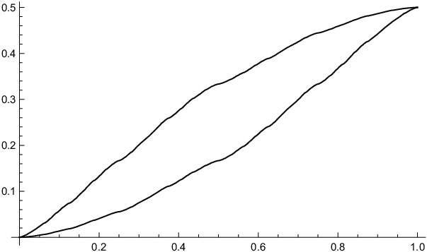
where the function f0f_{0} is Hölder continuous with exponent log2⁡(3/τ)\log_{2}(3/\tau). Moreover, f0​(t)f_{0}(t) is the first coordinate of the column vector f⁡(t)=(f0​(t),f1​(t))T{f}(t)=\bigl(f_{0}(t),f_{1}(t)\bigr)^{T} that is the unique solution of the dilation equation

f⁡(t)=13​(S0​f​(2​t)+S1​f​(2​t−1)),{f}(t)\,=\,\frac{\raisebox{-2.0pt}{$1$}}{\raisebox{0.5pt}{$3$}}\hskip 0.5pt\bigl({S}_{0}\hskip 0.5pt{f}(2t)+{S}_{1}\hskip 0.5pt{f}(2t-1)\bigr),

with the conditions f0​(t)=f1​(t)=0f_{0}(t)=f_{1}(t)=0 for t⩽0t\leqslant 0 and f0​(t)=f1​(t)=12f_{0}(t)=f_{1}(t)=\frac{1}{2} for t⩾1t\geqslant 1.

Sketch of proof.

This result follows from a method of Dumas. In particular, it follows from an application of [9, Thm. 3], when using the linear representation of the Stern sequence (1.3) along with the facts that the set {S0,S1}\{{S}_{0},{S}_{1}\} satisfies the finiteness property with joint spectral radius equal to the golden ratio (see [7, 8]), that Q:=S0+S1{Q}:={S}_{0}+{S}_{1} has eigenvalues 33 and 11 with Jordan basis v3=(12,12)T{v}_{3}=\bigl(\frac{1}{2},\frac{1}{2}\bigr)^{T} and v1=(12,−12)T{v}_{1}=\bigl(\frac{1}{2},-\frac{1}{2}\bigr)^{T}, and that v=v3+v1{v}={v}_{3}+{v}_{1}. ∎

Refer to caption
Figure 3. The functions f0f_{0} (lower curve) and f1f_{1} (upper curve).
Theorem 3.2.

The distribution function FF from Eq. (3.1) is strictly increasing.

Proof.

Let x∈[0,1)x\in[0,1) and ε>0\varepsilon>0 with x+ε⩽1x+\varepsilon\leqslant 1 be arbitrary. Since FF is continuous and non-decreasing, we have that

F⁡(x+ε)−F⁡(x)=μ⁡([0,x+ε])−μ⁡([0,x])=μ⁡([x,x+ε])⩾ 0.F(x+\varepsilon)-F(x)\,=\,\mu([0,x+\varepsilon])-\mu([0,x])\,=\,\mu([x,x+\varepsilon])\,\geqslant\,0\hskip 0.5pt.

Thus, to prove the theorem, it is enough to show that μ⁡([x,x+ε])>0\mu([x,x+\varepsilon])>0. Note also that, since the dyadic rationals are dense in [0,1][0,1], there exist positive integers mm and kk so that [2​m/2k,(2​m+1)/2k]⊆[x,x+ε][2m/2^{k},(2m+1)/2^{k}]\subseteq[x,x+\varepsilon]. Thus, to show that μ⁡([x,x+ε])>0\mu([x,x+\varepsilon])>0, it suffices to show that μ⁡([2​m/2k,(2​m+1)/2k])>0\mu([2m/2^{k},(2m+1)/2^{k}])>0.

To this end, observe that, for any real number y∈[2n,2n+1)y\in[2^{n},2^{n+1}), we have ⌊log2⁡(y)⌋=n\lfloor\log_{2}(y)\rfloor=n. Thus, combining Eq. (1.5) with Proposition 3.1 gives

μn​([2​m/2k,(2​m+1)/2k])\displaystyle\mu_{n}\bigl([2m/2^{k},(2m+1)/2^{k}]\bigr) = 3−n​∑ℓ=2n+2n​(2​m/2k)2n+2n​((2​m+1)/2k)s⁡(ℓ)\displaystyle=\,3^{-n}\sum_{\ell=2^{n}+2^{n}(2m/2^{k})}^{2^{n}+2^{n}((2m+1)/2^{k})}s(\ell)
= 3​f0​(2⟨log2⁡(2n+2n​((2​m+1)/2k))⟩−1)−3​f0​(2⟨log2⁡(2n+2n​(2​m/2k))⟩−1)\displaystyle=\,3\hskip 0.5ptf_{0}\big(2^{\langle\log_{2}(2^{n}+2^{n}((2m+1)/2^{k}))\rangle-1}\big)-3\hskip 0.5ptf_{0}\big(2^{\langle\log_{2}(2^{n}+2^{n}(2m/2^{k}))\rangle-1}\big)
+On​(3−n​(2n+2n​((2​m+1)/2k))log2⁡(τ)+ε),\displaystyle\qquad\qquad+O_{n}\left(3^{-n}\bigl(2^{n}+2^{n}((2m+1)/2^{k})\bigr)^{\log_{2}(\tau)+\varepsilon}\right),

where we have used the notation OnO_{n} to indicate the dependence on nn. Since mm and kk are fixed, one has

On​((2n+2n​((2​m+1)/2k))log2⁡(τ)+ε​ 3−n)=On​(2n⁡(log2⁡(τ)+ε)​ 3−n)=on​(1),as n→∞,O_{n}\big((2^{n}+2^{n}((2m+1)/2^{k}))^{\log_{2}(\tau)+\varepsilon}\,3^{-n}\big)\,=\,O_{n}\big(2^{n(\log_{2}(\tau)+\varepsilon)}\,3^{-n}\big)\,=\,o_{n}(1)\hskip 0.5pt,\quad\text{as $n\to\infty$,}

and, for any y∈(0,1)y\in(0,1),

⟨log2⁡(2n+2n​y)⟩=⟨n+log2⁡(1+y)⟩=log2⁡(1+y).\langle\log_{2}(2^{n}+2^{n}y)\rangle\,=\,\langle n+\log_{2}(1+y)\rangle\,=\,\log_{2}(1+y)\hskip 0.5pt.

Continuing the above then gives

μn​([2​m/2k,(2​m+1)/2k])= 3​f0​(((2​m+1)/2k)+12)−3​f0​((2​m/2k)+12)+on​(1).\mu_{n}\bigl([2m/2^{k},(2m+1)/2^{k}]\bigr)\,=\,3\hskip 0.5ptf_{0}\left(\frac{((2m+1)/2^{k})+1}{2}\right)-3\hskip 0.5ptf_{0}\left(\frac{(2m/2^{k})+1}{2}\right)+o_{n}(1)\hskip 0.5pt.

Taking the limit as nn goes to infinity gives

(3.2) μ⁡([2​m/2k,(2​m+1)/2k])= 3​f0​(2k+2​m+12k+1)−3​f0​(2k+2​m2k+1).\mu\bigl([2m/2^{k},(2m+1)/2^{k}]\bigr)\,=\,3\hskip 0.5ptf_{0}\Bigl(\frac{\raisebox{-2.0pt}{$2^{k}+2m+1$}}{\raisebox{0.5pt}{$2^{k+1}$}}\Bigr)-3\hskip 0.5ptf_{0}\Bigl(\frac{\raisebox{-2.0pt}{$2^{k}+2m$}}{\raisebox{0.5pt}{$2^{k+1}$}}\Bigr).

We can now use the dilation equation for f{f} to determine the value of the right-hand side of (3.2) based on the binary expansion of the numerators of the dyadic rationals involved. In particular, if bi∈{0,1}b_{i}\in\{0,1\} for i∈{0,1,…,k}i\in\{0,1,\ldots,k\}, we have

f(bk​2k+bk−1​2k−1+⋯+b1​2+b02k+1)={16​(1011)​(11)+13​(1101)​f​(bk−1​2k−1+⋯+b1​2+b02k),if bk=113​(1011)​f​(bk−1​2k−1+⋯+b1​2+b02k),if bk=0=bk6​(1011)​(11)+[bk3​(1101)+1−bk3​(1011)]​f​(bk−1​2k−1+⋯+b1​2+b02k)=bk6​(1011)​(11)+13​(1101)bk​(1011)1−bk​f​(bk−1​2k−1+⋯+b1​2+b02k).\begin{split}{f}&\left(\frac{b_{k}2^{k}+b_{k-1}2^{k-1}+\cdots+b_{1}\hskip 0.5pt2+b_{0}}{2^{k+1}}\right)\\[8.53581pt] &\quad\quad=\,\left\{\begin{array}[]{ll}\dfrac{1}{6}\left(\begin{matrix}1&0\\ 1&1\end{matrix}\right)\left(\begin{matrix}1\\ 1\end{matrix}\right)+\dfrac{1}{3}\left(\begin{matrix}1&1\\ 0&1\end{matrix}\right){f}\left(\dfrac{b_{k-1}2^{k-1}+\cdots+b_{1}\hskip 0.5pt2+b_{0}}{2^{k}}\right),&\mbox{if $b_{k}=1$}\\[14.22636pt] \dfrac{1}{3}\left(\begin{matrix}1&0\\ 1&1\end{matrix}\right){f}\left(\dfrac{b_{k-1}2^{k-1}+\cdots+b_{1}\hskip 0.5pt2+b_{0}}{2^{k}}\right),&\mbox{if $b_{k}=0$}\end{array}\right.\\[8.53581pt] &\quad\quad=\dfrac{b_{k}}{6}\left(\begin{matrix}1&0\\ 1&1\end{matrix}\right)\left(\begin{matrix}1\\ 1\end{matrix}\right)+\left[\dfrac{b_{k}}{3}\left(\begin{matrix}1&1\\ 0&1\end{matrix}\right)+\dfrac{1-b_{k}}{3}\left(\begin{matrix}1&0\\ 1&1\end{matrix}\right)\right]{f}\left(\dfrac{b_{k-1}2^{k-1}+\cdots+b_{1}\hskip 0.5pt2+b_{0}}{2^{k}}\right)\\[8.53581pt] &\quad\quad=\dfrac{b_{k}}{6}\left(\begin{matrix}1&0\\ 1&1\end{matrix}\right)\left(\begin{matrix}1\\ 1\end{matrix}\right)+\dfrac{1}{3}\left(\begin{matrix}1&1\\ 0&1\end{matrix}\right)^{b_{k}}\left(\begin{matrix}1&0\\ 1&1\end{matrix}\right)^{1-b_{k}}{f}\left(\dfrac{b_{k-1}2^{k-1}+\cdots+b_{1}\hskip 0.5pt2+b_{0}}{2^{k}}\right).\end{split}

Note next that

(1101)bk​(1011)1−bk=Sbk,\left(\begin{matrix}1&1\\ 0&1\end{matrix}\right)^{b_{k}}\left(\begin{matrix}1&0\\ 1&1\end{matrix}\right)^{1-b_{k}}=\,{S}_{b_{k}}\hskip 0.5pt,

where Sbk{S}_{b_{k}} is as given in the linear representation of s⁡(n)s(n). Thus setting

ubk:=bk2​(1011)​(11)=bk2​(12),{u}_{b_{k}}\,:=\,\dfrac{b_{k}}{2}\left(\begin{matrix}1&0\\ 1&1\end{matrix}\right)\left(\begin{matrix}1\\ 1\end{matrix}\right)\,=\,\dfrac{b_{k}}{2}\left(\begin{matrix}1\\ 2\end{matrix}\right),

we have

(3.3) (f⁡(bk​2k+⋯+b1​2+b02k+1)1)=13​(Sbkubk0 03)​(f⁡(bk−1​2k−1+⋯+b1​2+b02k)1).\left(\begin{matrix}{f}\left(\frac{b_{k}2^{k}+\cdots+b_{1}2+b_{0}}{2^{k+1}}\right)\\ 1\end{matrix}\right)=\frac{\raisebox{-2.0pt}{$1$}}{\raisebox{0.5pt}{$3$}}\left(\begin{matrix}{S}_{b_{k}}&{u}_{b_{k}}\\ 0\ \ \ 0&3\end{matrix}\right)\left(\begin{matrix}{f}\left(\frac{b_{k-1}2^{k-1}+\cdots+b_{1}2+b_{0}}{2^{k}}\right)\\ 1\end{matrix}\right).

Iterating Eq. (3.3) we get

(3.4) (f⁡(bk​2k+⋯+b1​2+b02k+1)1)=13k(Sbkubk0 03)⋯(Sb1ub10 03)(f⁡(b02)1).\left(\begin{matrix}{f}\left(\frac{b_{k}2^{k}+\cdots+b_{1}2+b_{0}}{2^{k+1}}\right)\\ 1\end{matrix}\right)=\frac{\raisebox{-2.0pt}{$1$}}{\raisebox{0.5pt}{$3^{k}$}}\left(\begin{matrix}{S}_{b_{k}}&{u}_{b_{k}}\\ 0\ \ \ 0&3\end{matrix}\right)\cdots\left(\begin{matrix}{S}_{b_{1}}&{u}_{b_{1}}\\ 0\ \ \ 0&3\end{matrix}\right)\left(\begin{matrix}{f}\left(\frac{b_{0}}{2}\right)\\ 1\end{matrix}\right).

For the integer 2​m∈[0,2k)2m\in[0,2^{k}), consider the binary expansions 2k+2m+1=1bk−1⋯b112^{k}+2m+1=1b_{k-1}\cdots b_{1}1 and 2k+2m=1bk−1⋯b102^{k}+2m=1b_{k-1}\cdots b_{1}0 in obvious notation. Then, using Eqs. (3.2) and (3.4) and observing that f⁡(12)=(16,13)Tf\bigl(\frac{1}{2}\bigr)=\bigl(\frac{1}{6},\frac{1}{3}\bigr)^{T}, we have

μ([2m/2k,(2m+1)/2k)])\displaystyle\mu([2m/2^{k},(2m+1)/2^{k})])\, =(31−k,0,0)(S1u10 03)⋯(Sb1ub10 03)[(f⁡(12)1)−(f⁡(0)1)]\displaystyle=\,(3^{1-k},0,0)\left(\begin{matrix}{S}_{1}&{u}_{1}\\ 0\ \ \ 0&3\end{matrix}\right)\cdots\left(\begin{matrix}{S}_{b_{1}}&{u}_{b_{1}}\\ 0\ \ \ 0&3\end{matrix}\right)\left[\left(\begin{matrix}{f}\left(\frac{1}{2}\right)\\ 1\end{matrix}\right)-\left(\begin{matrix}{f}\left(0\right)\\ 1\end{matrix}\right)\right]
=16(31−k,0,0)(S1u10 03)⋯(Sb1ub10 03)(120)\displaystyle=\,\frac{\raisebox{-2.0pt}{$1$}}{\raisebox{0.5pt}{$6$}}(3^{1-k},0,0)\left(\begin{matrix}{S}_{1}&{u}_{1}\\ 0\ \ \ 0&3\end{matrix}\right)\cdots\left(\begin{matrix}{S}_{b_{1}}&{u}_{b_{1}}\\ 0\ \ \ 0&3\end{matrix}\right)\left(\begin{matrix}1\\ 2\\ 0\end{matrix}\right)
=16(31−k,0)S1Sbk−1⋯Sb1(12)⩾36⋅3k> 0,\displaystyle=\,\frac{\raisebox{-2.0pt}{$1$}}{\raisebox{0.5pt}{$6$}}(3^{1-k},0)\,{S}_{1}\,{S}_{b_{k-1}}\,\cdots\,{S}_{b_{1}}\left(\begin{matrix}1\\ 2\end{matrix}\right)\,\geqslant\,\frac{\raisebox{-2.0pt}{$3$}}{\raisebox{0.5pt}{$6\cdot 3^{k}$}}\,>\,0\hskip 0.5pt,

which proves the theorem. ∎

Unlike other distribution functions of singular continuous measures, the distribution function FF from Eq. (3.1) looks relatively ‘smooth’; this is quantified in the following corollary.

Corollary 3.3.

The distribution function FF from Eq. (3.1) is Hölder continuous with exponent log2⁡(3/τ)\log_{2}(3/\tau).

Proof.

The distribution function FF inherits this exponent from the dilation equation for the assiciated function ff. One can see this by following through the proof of Theorem 3.2 up to Eq. (3.2) using the interval [x,y]⊆[0,1][x,y]\subseteq[0,1]. ∎

Further, it will be an interesting question to analyse some of the scaling properties of μ\mu, for instance in analogy to the treatment of the Thue–Morse measure in [5]. For this, it will be helpful to understand the precise relation between the measure μ\mu and the dilation equation from Proposition 3.1. One such relation can be stated as follows.

Corollary 3.4.

For x∈[0,1]x\in[0,1], the distribution function FF from Eq. (3.1) satisfies

F⁡(x)= 3​(f0​(1+x2)−f0​(12))=f0​(x)+f1​(x),F(x)\,=\,3\left(f_{0}\bigl(\tfrac{1+x}{2}\bigr)-f_{0}\bigl(\tfrac{1}{2}\bigr)\right)\,=\,f_{0}(x)+f_{1}(x)\hskip 0.5pt,

where f0f_{0} and f1f_{1} are the functions from Proposition 3.1.

Proof.

The first identity is a rather direct consequence of Eq. (3.2) in the proof of Proposition 3.1. While f0​(12)=16f_{0}\bigl(\frac{1}{2}\bigr)=\frac{1}{6}, the dilation equation for the functions fif_{i} gives

f0​(1+x2)=16+13​(f0​(x)+f1​(x)).f_{0}\bigl(\tfrac{1+x}{2}\bigr)\,=\,\frac{\raisebox{-2.0pt}{$1$}}{\raisebox{0.5pt}{$6$}}+\frac{\raisebox{-2.0pt}{$1$}}{\raisebox{0.5pt}{$3$}}\bigl(f_{0}(x)+f_{1}(x)\bigr).

This implies the second identity. ∎

Appendix

The purpose of this appendix is to provide two other proofs of the continuity of the measure μ\mu from Proposition 2.2, in view of their potential usefulness in other applications to recursive sequences of a similar kind.

The first one starts from the observation that μ=∗m⩾1νm\mu=\raisebox{-2.5pt}{\mbox{\huge$*$}}_{m\geqslant 1}\nu_{m}, with the probability measures νm=13​(δ0+δ2−m+δ−2−m)\nu_{m}=\frac{1}{3}\bigl(\delta_{0}+\delta_{2^{-m}}+\delta_{-2^{-m}}\bigr) on 𝕋\mathbb{T} as building blocks, is absolutely convergent in the weak topology, which is to say that that it is weakly convergent to the same limit in any order of its terms. This follows from [12, Thm. 6], where one has to notice that

Mr​(νm):=∫𝕋xr​d​νm​(x)=13​(0r+2−r​m+(−1)r​2−r​m)M_{r}(\nu_{m})\,:=\int_{\mathbb{T}}x^{r}\,\mathrm{d}\nu_{m}(x)\,=\,\frac{\raisebox{-2.0pt}{$1$}}{\raisebox{0.5pt}{$3$}}\bigl(0^{r}+2^{-rm}+(-1)^{r}2^{-rm}\bigr)

for r⩾0r\geqslant 0. In particular, M1​(νm)=0M_{1}(\nu_{m})=0 and M2​(νm)=23​4−mM_{2}(\nu_{m})=\frac{2}{3}\hskip 0.5pt4^{-m}, so both ∑m=1∞|M1​(νm)|\sum_{m=1}^{\infty}\lvert M_{1}(\nu_{m})\rvert and ∑m=1∞M2​(νm)\sum_{m=1}^{\infty}M_{2}(\nu_{m}) are finite, which ensures absolute convergence.

If we now assume, contrary to the claim, that μ\mu fails to be continuous, there must be an x∈𝕋x\in\mathbb{T} with μ⁡({x})>0\mu(\{x\})>0. Now, rewrite μ\mu as μ=νn∗ρn\mu=\nu_{n}*\rho_{n} with ρn:=∗m≠nνm\rho_{n}:=\raisebox{-2.5pt}{\mbox{\huge$*$}}_{m\neq n}\nu_{m}, which is possible for any n∈ℕn\in\mathbb{N}. This implies

μ⁡({x})=(νn∗ρn)​({x})=13​(ρn​({x})+ρn​({x+2−n})+ρn​({x−2−n})).\mu(\{x\})\,=\,\bigl(\nu_{n}*\rho_{n}\bigr)(\{x\})\,=\,\frac{\raisebox{-2.0pt}{$1$}}{\raisebox{0.5pt}{$3$}}\bigl(\rho_{n}(\{x\})+\rho_{n}(\{x+2^{-n}\})+\rho_{n}(\{x-2^{-n}\})\bigr).

Analogously, one obtains

μ⁡({x±2−n})=13​(ρn​({x})+ρn​({x±2−n})+ρn​({x±2⋅2−n})).\mu(\{x\pm 2^{-n}\})\,=\,\frac{\raisebox{-2.0pt}{$1$}}{\raisebox{0.5pt}{$3$}}\bigl(\rho_{n}(\{x\})+\rho_{n}(\{x\pm 2^{-n}\})+\rho_{n}(\{x\pm 2\cdot 2^{-n}\})\bigr).

Together with the previous relation, this implies the estimate22 2 More generally, one has the relation νn⩽(δ2−n+δ−2−n)∗νn\nu_{n}\leqslant\bigl(\delta_{2^{-n}}+\delta_{-2^{-n}}\bigr)*\nu_{n} as an inequality between positive measures, and hence — by convolution with ρn\rho_{n} — also μ⩽(δ2−n+δ−2−n)∗μ\mu\leqslant\bigl(\delta_{2^{-n}}+\delta_{-2^{-n}}\bigr)*\mu, which implies Eq. (3.5).

(3.5) μ⁡({x})⩽μ⁡({x+2−n})+μ⁡({x−2−n}).\mu(\{x\})\,\leqslant\,\mu(\{x+2^{-n}\})+\mu(\{x-2^{-n}\})\hskip 0.5pt.

Now, choose r∈ℕr\in\mathbb{N} with μ⁡({x})>1r\mu(\{x\})>\frac{1}{r}, and select rr integers j1<j2<…<jrj_{1}<j_{2}<\ldots<j_{r} with j1⩾2j_{1}\geqslant 2. Since μ\mu is a probability measure on 𝕋\mathbb{T}, we then get

1⩾μ⁡(⋃1⩽q⩽r˙​({x−2−jq}​∪˙​{x+2−jq}))=∑q=1r(μ⁡({x−2−jq})+μ⁡({x+2−jq}))>r​μ​({x})⩾r​1r= 1.\begin{split}1\,&\geqslant\,\mu\biggl(\dot{\bigcup_{1\leqslant q\leqslant r}}\bigl(\big\{x-2^{-j_{q}}\big\}\,\dot{\cup}\,\big\{x+2^{-j_{q}}\big\}\bigr)\biggr)\\ &=\,\sum_{q=1}^{r}\Bigl(\mu\bigl(\big\{x-2^{-j_{q}}\big\}\bigr)+\mu\bigl(\big\{x+2^{-j_{q}}\big\}\bigr)\Bigr)\,>\,r\hskip 0.5pt\mu\bigl(\{x\}\bigr)\;\geqslant\>r\,\frac{\raisebox{-2.0pt}{$1$}}{\raisebox{0.5pt}{$r$}}\;=\;1\hskip 0.5pt.\end{split}

This contradiction shows that μ\mu is continuous.

The second alternative proof employs Wiener’s criterion again. Observing (without proof) that the inequalities

(3.6) |μ^​(2​k+1)|⩽12​|μ^​(k)+μ^​(k+1)|andμ^​(2​k+1)​(μ^​(2​k)+μ^​(2​k+2))⩽ 0\lvert\widehat{\mu}(2k+1)\rvert\,\leqslant\,\frac{1}{2}\lvert\widehat{\mu}(k)+\widehat{\mu}(k+1)\rvert\quad\text{and}\quad\widehat{\mu}(2k+1)\bigl(\widehat{\mu}(2k)+\widehat{\mu}(2k+2)\bigr)\,\leqslant\,0

hold for all k∈ℤk\in\mathbb{Z}, one can proceed as follows. With Σ⁡(N):=∑k=−NNμ^​(k)2\varSigma(N):=\sum_{k=-N}^{N}\widehat{\mu}(k)^{2}, one has

Σ⁡(4​N)=∑k=−2​N2​Nμ^​(2​k)2+∑k=−2​N2​N−1μ^​(2​k+1)2⩽Σ⁡(2​N)+14​∑k=−2​N2​N−1(μ^​(k)+μ^​(k+1))2=32​Σ​(2​N)−μ^​(2​N)22+12​∑k=−2​N2​N−1μ^​(k)​μ^​(k+1)⩽32​Σ​(2​N)+12​∑k=−NN−1μ^​(2​k+1)​(μ^​(2​k)+μ^​(2​k+2))⩽32​Σ​(2​N),\begin{split}\varSigma(4N)\,&=\sum_{k=-2N}^{2N}\widehat{\mu}(2k)^{2}\,+\!\sum_{k=-2N}^{2N-1}\widehat{\mu}(2k+1)^{2}\,\leqslant\,\varSigma(2N)\,+\,\frac{\raisebox{-2.0pt}{$1$}}{\raisebox{0.5pt}{$4$}}\sum_{k=-2N}^{2N-1}\bigl(\widehat{\mu}(k)+\widehat{\mu}(k+1)\bigr)^{2}\\ &=\,\frac{\raisebox{-2.0pt}{$3$}}{\raisebox{0.5pt}{$2$}}\varSigma(2N)\,-\,\frac{\raisebox{-2.0pt}{$\widehat{\mu}(2N)^{2}$}}{\raisebox{0.5pt}{$2$}}\,+\,\frac{\raisebox{-2.0pt}{$1$}}{\raisebox{0.5pt}{$2$}}\sum_{k=-2N}^{2N-1}\widehat{\mu}(k)\,\widehat{\mu}(k+1)\\ &\leqslant\,\frac{\raisebox{-2.0pt}{$3$}}{\raisebox{0.5pt}{$2$}}\varSigma(2N)\,+\,\frac{\raisebox{-2.0pt}{$1$}}{\raisebox{0.5pt}{$2$}}\sum_{k=-N}^{N-1}\widehat{\mu}(2k+1)\bigl(\widehat{\mu}(2k)+\widehat{\mu}(2k+2)\bigr)\,\leqslant\,\frac{\raisebox{-2.0pt}{$3$}}{\raisebox{0.5pt}{$2$}}\varSigma(2N)\hskip 0.5pt,\end{split}

where Lemma 2.3 was used several times, while Eq. (3.6) was needed for the first and the last inequality.

This estimate implies Σ⁡(2k+1)⩽(32)k​Σ​(2)\varSigma(2^{k+1})\leqslant\bigl(\frac{3}{2}\bigr)^{k}\varSigma(2) and thus also Σ⁡(N)⩽C​(32)log2⁡(N)\varSigma(N)\leqslant C\hskip 0.5pt(\frac{3}{2})^{\log_{2}(N)} for some positive constant CC. With α=log2⁡(3/2)<1\alpha=\log_{2}(3/2)<1, one then obtains the asymptotic behaviour 1N​Σ​(N)=O⁡(1/N1−α)\frac{1}{N}\varSigma(N)=O(1/N^{1-\alpha}) as N→∞N\to\infty, which implies the absence of pure point components in μ\mu by Wiener’s criterion. This approach has the advantage (over the Jessen–Wintner argument) that one also gets a lower bound on the Hölder exponent from Corollary 3.3

Acknowledgements

It is our pleasure to thank Uwe Grimm, Jeff Hogan, Björn Rüffer, Timo Spindeler and Wadim Zudilin for helpful discussions. This work was supported by the German Research Council (DFG), within the CRC 701, and by the Australian Research Council, through grant DE140100223.

References

  • [1] Allouche J-P and Shallit J, The ring of kk-regular sequences, Theor. Comput. Sci. 98 (1992) 163–197.
  • [2] Baake M, Gähler F and Grimm U, Spectral and topological properties of a family of generalised Thue–Morse sequences, J. Math. Phys. 53 (2012) 032701 (24pp); arXiv:1201.1423.
  • [3] Baake M and Grimm U, Aperiodic Order. Vol. 1: A Mathematical Invitation, Cambridge University Press, Cambridge (2013).
  • [4] Baake M and Grimm U, Squirals and beyond: Substitution tilings with singular continuous spectrum, Ergodic Th. & Dynam. Syst. 34 (2014) 1077–1102; arXiv:1205.1384.
  • [5] Baake M, Grimm U and Nilsson J, Scaling of the Thue–Morse diffraction measure, Acta Phys. Pol. A 126 (2014) 431–434; arXiv:1311.4371.
  • [6] Berg C and Forst G, Potential Theory on Locally Compact Abelian Groups, Springer, Berlin (1975).
  • [7] Coons M, Regular sequences and the joint spectral radius, Intern. J. Found. Comput. Sci. 28 (2017) 135–140; arXiv:1511.07535.
  • [8] Coons M and Tyler J, The maximal order of Stern’s diatomic sequence, Moscow J. Comb. Number Th. 4 (2014) 277–287; arXiv:1307.1521.
  • [9] Dumas P, Joint spectral radius, dilation equations, and asymptotic behavior of radix-rational sequences, Lin. Alg. Appl. 438 (2013) 2107–2126.
  • [10] Erdős P, On a family of symmetric Bernoulli convolutions, Amer. J. Math. 61 (1939) 974–976.
  • [11] Erdős P, On the smoothness properties of a family of Bernoulli convolutions, Amer. J. Math. 62 (1940) 180–186.
  • [12] Jessen B and Wintner A, Distribution functions and the Riemann zeta function, Trans. Amer. Math. Soc. 38 (1935) 48–88.
  • [13] Peres Y, Schlag W and Solomyak B, Sixty years of Bernoulli convolutions, in Fractal Geometry and Stochastics II, eds. Bandt S, Graf S and Zähle M, Birkhäuser, Basel (2000), pp. 39–65.
  • [14] Reiter H and Stegeman J D, Classical Harmonic Analysis and Locally Compact Groups, Clarendon Press, Oxford (2000).
  • [15] Sloane N J A (ed.), The On-Line Encyclopedia of Integer Sequences, available at https://oeis.org/