Gravitational lensing by scalar-tensor wormholes and the energy conditions
Abstract
We study gravitational lensing by a class of zero Ricci scalar wormholes which arise as solutions in a scalar-tensor theory of gravity. An attempt is made to find a possible link between lensing features, stable/unstable photon orbits and the energy conditions on the matter required to support these spacetimes. Our analysis shows (for this class of wormholes) that light rays always exhibit a positive deflection if the energy conditions are satisfied (nonexotic matter content). In contrast, if the energy conditions are violated (exotic matter), the net deflection of a light ray may be positive, negative or even zero, depending on values of the metric and impact parameters. This prompts us to introduce a surface defined by a turning point value at which the net deflection of a light ray is equal to zero, even though we have a curved spacetime geometry. We argue that the existence of such a surface may be linked to exotic/energy condition violating matter. Wormholes in modified gravity with matter satisfying the energy conditions do not seem to have such a zero deflection surface. Finally, we study strong gravitational lensing briefly and also look into the formation of Einstein and relativistic Einstein rings. We conclude with some estimates on the wormhole mass, throat-radius and the detectability of the Einstein rings.
I Introduction
Gravitational lensing is one of the observational probes of a given spacetime geometry and the gravitational field it represents. Theoretical prediction of light bending and its subsequent observational verification [1, 2] is celebrated as one of the successful tests of general relativity (GR) in the weak field limit. In modern astronomy and cosmology, gravitational lensing is widely used as an important tool for probing extrasolar planets, highly redshifted galaxies, quasars, supermassive black holes, dark matter candidates, primordial gravitational wave signatures, etc. [3, 4, 5]. It is also used to test the viability of different alternative theories of gravity [6].
After the observational confirmation of the bending of light, interest in studying gravitational lensing has grown immensely in the last few decades. Strong deflection of light rays by the simplest black hole, the Schwarzschild, was first studied in [7]. An exact analytic expression for the deflection angle by the Schwarzschild black hole was obtained in [8]. Subsequently, gravitational lensing by the Schwarzschild black hole in the strong field limit and various aspects (eg. formation of relativistic images, their magnification and critical curves) have been studied in [9, 10, 11, 12] in a systematic way. Bozza developed an analytic framework to study gravitational lensing for a completely generic, spherically symmetric, static spacetime in the strong field limit and applied it to some existing spacetimes [13, 14]. The study of gravitational lensing is not only limited to the Schwarzschild black hole. Lensing by other black holes such as Reissner-Nordstrm [15, 16, 17, 18], Kerr [19, 20, 21], Kiselev [22, 23], global monopole [24, 25, 26], Einstein-Born-Infeld [27], Eddington-Born-Infeld [28, 29, 30], scalar-tensor [31, 32], braneworld [33, 34, 35, 36], dilaton [37, 38, 39, 40], phantom [41, 42], regular [43, 44, 45, 46], Kaluza-Klein [47, 48, 49, 50], Horava-Lifshitz [51], Myers-Perry [52] and Galileon [53] black holes, have been studied. Gravitational lensing by naked singularities has been analyzed to see whether one can distinguish between a black hole and a naked singularity [54, 55, 56, 57, 58]. Such studies show that, in some cases, lensing by a naked singularity is qualitatively different from that by a black hole. Gravitational lensing [59, 60, 61, 62, 63, 64, 65, 66, 67, 68, 69, 70] and microlensing [71, 72, 73] by wormholes has been a topic of growing interest in the recent past too. It has been shown that gravitational lensing can be used as a distinguishing probe between black holes and wormholes [72, 74, 75].
However, the above-mentioned works are limited only to lensing features. Any possible link between lensing and matter content of a given spacetime geometry, has not been explored much. It may be noted that though gravitational lensing can be understood geometrically, the field equations of a given theory of gravity relates geometry to matter stress energy. Thus, gravitational lensing properties of a given spacetime geometry should, in principle, be related to the matter content of the spacetime. Attempts have been made to relate lensing with matter stress energy within the framework of GR [76, 77, 78]. In our work here, we explore the relation between lensing and matter content through a specific example of a geometry in on-brane scalar-tensor gravity. In particular, we study gravitational lensing by on-brane scalar-tensor wormholes obtained in [79]. It is well-known that wormholes in GR, violate the energy conditions. However, the modified or alternative gravity wormholes do not necessarily violate the energy conditions (see [80] for some recent examples and references therein). Depending on the parameter values, the wormholes in our study, may or may not violate the energy conditions. Therefore, it is of interest to explore whether there is any quantitative or qualitative difference between lensing by a wormhole satisfying the energy conditions and that for wormholes violating them.
Our paper is organized as follows. In Sec. II, we briefly recall the scalar-tensor wormholes and the corresponding energy conditions. In Sec. III, we study the existence of stable and unstable photon orbits and its relation with the energy conditions. Sections IV and V deal with gravitational lensing by the general wormholes. In Secs. VI and VII, we study the formation of Einstein and relativistic Einstein rings and their detectability. Finally, we conclude in Sec. VIII.
II R=0 wormholes and the energy conditions
The spacetime geometry obtained in [79] is given by
| (1) |
where and
| (2) |
The version of this geometry has been discussed in [81] and, more recently, in [82].
The equation which will be useful in our subsequent analysis is given by
| (3) |
In [79], the weak energy condition was studied by writing down the solution in isotropic coordinates. The transformation from the Schwarzschild radial coordinate to the isotropic coordinate is given as
| (4) |
The line element in isotropic coordinates, becomes
| (5) |
where
| (6) |
| (7) |
and
| (8) |
The constants and are given as
| (9) |
It is easy to show that and are related to and as follows:
| (10) |
In [79], we have shown that, in order to satisfy the weak energy condition, we must have, in the limit (i.e., ),
| (11) |
where is an integration constant related to the scalar field given by
| (12) |
Using Eqn. (11), it can be shown that, in the limit (i.e., for large ), the energy density , radial pressure and the tangential pressure (see [79] for the expressions of , and ) behave as
where
and . Therefore, asymptotically, matter energy-momentum resembles that due to a static electric field in Maxwell electrodynamics with playing the role of electric charge. In [79], we have also shown that, in the limit , the positivity of the leading-order term in (i.e., in the present work) ensures the satisfaction of the weak energy condition. However, there we set to zero and obtained another expression for (Eqn. (28) of [79]). By comparing the two expressions for , we obtained a relation between and . However, in the present work, we relax this condition and do not set to zero identically. We choose and independently in such a way that . This gives
| (13) |
which allows us to explore a wider range of the parameter space for which the weak energy condition holds. Note that the traceless condition implies . Hence, the satisfaction of the weak energy condition ensures the satisfaction of the strong and hence, all other energy conditions. The shaded region in Fig. 1 shows the parameter values for which the energy conditions are satisfied.

III Stable and unstable photon orbits and the energy conditions
The first integral obtained from the geodesic equations for a photon moving in the equatorial () plane of the spacetime in Eqn. (1) are given by
| (14) |
where the energy and the angular momentum are constants of motion. An overdot represents differentiation with respect to the parameter parametrizing the geodesics. The effective potential is given by
| (15) |
Circular photon orbits correspond to (i.e., ) and (i.e., extrema of the effective potential). Stable and unstable photon orbits correspond to the minimum () and maximum () of the effective potential, respectively. Defining , the effective potential can be rewritten as
| (16) |
where
| (17) |
and is the throat radius. The stable and unstable photon orbits still correspond to and , respectively. The extrema of the potential are given by
| (18) |
which becomes
| (19) |
Using Eqns. (3) and (18), it can be shown that [79]
| (20) |
Therefore, minima () exist if are real and . Note that we must have . This is possible when . Let us now put in Eqn. (19). We obtain
| (21) |
Note that at and as . Therefore, the ranges to have stable photon orbits, become and . Using Eqn. (21), one can show that is always negative ( for ) by plotting it as a function of . This implies that and become complex conjugates of each other. Therefore, stable photon orbit does not exist for real and satisfying the energy conditions. It may exist for imaginary and . Note that, for complex conjugate and , the metric functions, the energy density and pressures are real since and are real. It can also be shown that is real. To verify this, let and , where and are real. In terms of and , and become
| (22) |
Note that we must have since . We express and as
| (23) |
| (24) |
where . Therefore, becomes
| (25) |
which is real. To make positive, we must have since . This is achieved by taking the negative root of Eqn. (11), which becomes
| (26) |
where . In the limit , one can also express in terms of and . Figure 2 shows the parameter region where and and the region where the energy conditions are satisfied. The absence of an overlap region indicates that the energy conditions have to be violated for the parameter values required to have a stable photon orbit. Therefore, no stable photon orbit exists for the parameter values satisfying the energy conditions. However, as shown in [79], unstable photon orbits (photon spheres) exist for parameter values satisfying the energy conditions.

IV Gravitational lensing by the wormholes and the energy conditions
Let us now see how the wormholes affect light rays. We begin with a general spherically symmetric, static spacetime given by
| (27) |
The first integrals obtained from the geodesic equations for a photon moving in the equatorial plane ( plane) are given by
| (28) |
Therefore, we obtain
| (29) |
where is the impact parameter. At the turning point , . This gives the following relationship between the impact parameter and the turning point :
| (30) |
Therefore, the exact expression for deflection angle can be written as [83]
| (31) |
where
| (32) |
and
| (33) |
It is difficult to perform the above integration for the general metric. The case and gives the ultrastatic Schwarzschild wormhole. In this case, we put in the integral. We obtain
| (34) | |||||
where is an elliptic function of first kind. For the general case, we have to perform the integration numerically. Figure 3 shows the plots for the deflection angle, obtained numerically for different values of the metric parameters. It should be noted that the deflection angle is negative for some parameter values. A negative deflection angle has also been obtained in gravitational lensing by a naked singularity [54]. To visualize the negative deflection, we solve the geodesic equation and plot the light trajectories in Fig. 4. The negatively deflected light rays are deflected away from the wormhole. Note that, for some parameter values, there is a turning point for which the net deflection angle becomes zero. We denote this turning point by . We name this as a surface of zero deflection in the sense that any light ray which comes from infinity, turns at the surface of radius and then goes to infinity without taking any turn around the wormhole lens, does not undergo any net deflection by the background gravitational field. This scenario is achieved if the light ray undergoes both positive and negative deflection (so that the net is zero) along its path. Figure 5 shows the equatorial trajectory of a light ray undergoing zero net deflection.


From Fig. 3, it is clear that the deflection angle for all turning points always remain positive if the weak deflection is positive. Therefore, it is useful to obtain an exact expression for the deflection angle in the weak field limit and identify the parameter region where such negative deflection occurs. The radial component of the null geodesic equation can be written as
Using the inverse radial coordinates and , the above equation can be written in the form [84]
| (35) |
In our case,
where . For small deflection, we solve the above equation perturbatively. For small , we obtain
| (36) |
where
We now define a smallness parameter , where is the inverse of the Newtonian distance of closest approach. Therefore, in terms of the dimensionless variable , Eqn. (36) yields
| (37) |
Expanding as , we obtain the following order by order equations
Solving these equations, we finally arrive at
where it is assumed that the light source is at . For small deflection, we have and at spatial infinity. The deflection angle () is given by
| (38) |
At the turning point , . This gives the following relation between and :
| (39) |
In terms of , the deflection angle becomes
| (40) | |||||
In the limit , and , we recover the Reissner-Nordstrm spacetime. Therefore, the deflection angle, in this limit, becomes
| (41) |
which is the same as that obtained in [85]. In terms of the constants and , the weak deflection angle can be written as
| (42) |
It is to be noted that, in addition to the weak lensing by Schwarzschild mass (ADM mass), the naked singularities have positive () and wormhole solutions have negative () contribution to the first-order weak deflection. The first-order weak deflection angle is positive for , i.e., . For parameters not respecting this inequality, the weak deflection angle becomes negative.


Figure 6 shows the parameter regions for which the deflection angle is positive and the energy conditions are satisfied. It is clear that the deflection angle is always (i.e., for all impact parameters) positive for the parameter values satisfying the energy conditions. However, for the parameter values violating the energy conditions, the deflection angle can either be positive or negative depending on the impact parameter value. Figure 7 shows a comparison between the numerically obtained deflection angle and that found for weak deflection. For , the matching of the two curves is reasonably good, including the location of the turning point where zero deflection occurs. We mentioned earlier that the surface of zero deflection is achieved if the light ray undergoes both positive and negative deflection (so that the net is zero) along its path. Our analysis therefore indicates that the energy conditions must be violated to have a surface of zero deflection. Therefore, the existence of such a surface may be linked to the exotic matter (energy condition violating matter) content of the wormholes. If matter satisfies the energy conditions, such a zero deflection surface will not exist.
V Gravitational lensing in the strong deflection limit
In the previous section, we have seen that the deflection angle may become negative. Therefore, it is useful to see what happens to the deflection angle in the strong deflection limit. To study gravitational lensing in the strong deflection limit, we follow the analysis given by Bozza [13]. With the definition of two new variables
| (43) |
where , the integral in the deflection angle becomes
| (44) |
where
| (45) |
and
| (46) |
The term is regular for all and . But, diverges at , i.e., at . In the limit , can be written as
| (47) |
where
| (48) |
| (49) |
For the general metric (27), the photon sphere radius is given by . Note that vanishes at the photon sphere. Therefore, as the turning point approaches the photon sphere , diverges logarithmically. To show this, we split into a divergent part and a regular part as
| (50) |
where
| (51) |
and
| (52) |
After following the steps of [13], the deflection angle in the strong deflection limit can be written as
| (53) |
where
| (54) |
| (55) |
| (56) |
In terms of the angular diameter of the relativistic images, the deflection angle can be written as
| (57) |
where
| (58) |
Here, is the distance between the observer and the lens (see Fig. 10). is the minimum impact parameter given by . For the light rays passing very close to the photon sphere , where is the winding number. Therefore, the angular diameter of the relativistic image is given by
| (59) |
where . One of the observables is the angular separation between the outermost relativistic image () and the inner ones [13]. We have
| (60) |
Using Eqns. (3) and (18), we obtain, for the metric (1),
| (61) |
where and , being the solution of Eqn. (19). We find numerically and plot in Fig. 8 for real and . Note that the relativistic images for the parameter values satisfying the energy conditions are less closely spaced than those for the parameter values violating the energy conditions. Figure 9 shows the plot of for arbitrarily chosen and for which and may become complex conjugate to each other.

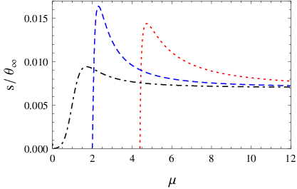
It should be noted that, in the limit , approaches a constant value. This can also be shown analytically. In the limit (i.e., ), the metric becomes the extremal Reissner-Nordstrm spacetime given by
| (62) |
For this metric, we find that , and
| (63) |
The above integration can be done analytically if we put . After performing the integration, we find that
| (64) |
Therefore, we find that , which matches with that in Fig. 9.
VI Einstein and relativistic Einstein rings
In this section, we find the angular diameter of the Einstein and relativistic Einstein rings. The lensing configuration is shown in Fig. 10.

When the observer and the source are far away from the lens, i.e., when and (thin lens approximation), the lens equation becomes
| (65) |
where, . Note that we have assumed , and . For a ring image, we set . As the turning point approaches the photon sphere, the light rays wind around the lens many times. In general, the deflection angle can be expressed as . In the weak field limit (), the winding number should be zero, thereby giving the Einstein ring. Therefore, the angular diameter of the Einstein ring is given by
| (66) |
where is the weak deflection given in Eqn. (42). Relativistic Einstein rings are formed by the light rays passing very close to the photon sphere and there are a large number (theoretically, an infinite number) of such rings. In the previous section, we have seen that these relativistic images are closely spaced. Here, we consider relativistic rings forming a single ring image [10, 74]. For such rings, the relation is satisfied for [74] (since is small). We may take , and the critical impact parameter is given by . Therefore, the angular diameters of the relativistic Einstein rings become
| (67) |
We then find out the expressions for the angular diameter and and establish a relationship between them. Note that, in order to obtain the diameter angles and the relationship between them, we need an analytic expression for the photon sphere radius which is difficult to obtain for the general wormhole geometries. Therefore, we concentrate on the special case . In this case, the first-order weak deflection angle is given by
| (68) |
The first-order weak deflection is negative for . For , the angular diameter of the Einstein ring is given by (see Eqn. (66))
| (69) |
However, the first-order weak deflection is zero for . In this case, we have to consider the second-order term which is . Therefore, the angular diameter is given by
| (70) |
To find the angular diameter of the relativistic Einstein rings, we need to find the photon sphere radius by solving Eqn. (19) for . For , we obtain
| (71) |
The photon sphere does not exist for . We recover the photon sphere radius of the Schwarzschild black hole for . It tends to as . After some manipulation, we obtain the critical impact parameter
| (72) |
for light rays winding around the photon sphere. For large , we recover the critical impact parameter of the Schwarzschild black hole. However, for , the photon sphere does not exist and the deflection angle diverges as approaches the wormhole throat . In that case, we take to calculate the critical impact parameter which becomes . Therefore, the angular diameters of the relativistic Einstein rings become
| (73) |
The relationship between and turns out to be
Thus, the qualitative feature of lensing for is different from that for .
VII Detectability of rings and wormhole size
The authors in [74] have shown that one can detect the relativistic Einstein rings formed by an Ellis-Bronnikov wormhole (i) with throat radius pc at a Galactic center and distance Mpc and (ii) with throat radius 10 AU in our Galaxy and distance kpc, using the most powerful modern instruments which have resolution of arcsecond (such as a 10-meter optical-infrared telescope). In order to detect the relativistic Einstein rings by a telescope with resolution of arcsecond, the minimum angular diameter of the relativistic rings should be of the order of arcsecond.
What is the scenario of a similar detection possibility of these rings which may be formed by the type of wormholes discussed in this article? Notice that for our wormholes, we have a parameter as well as . Using Eqn. (73), we find that, for a wormhole (of the class discussed here) at a Galactic center with Mpc, the minimum throat size () should lie between 0.97 pc and 0.34 pc for . One can calculate the corresponding mass of the wormhole using . This turns out to be in the range between and for , being the mass of the Sun. However, to detect the relativistic Einstein rings produced by such a wormhole at the center of our Galaxy with kpc, the throat size should lie between AU and AU for . The corresponding mass of the wormhole turns out to be in the range between and for . The above results for these wormholes are therefore similar, in terms of mass, to those for supermassive black holes [74].
It may be noted that one can find the wormhole parameters and once , , and are given. Figure 11 shows (in arcseconds) the angle of the relativistic Einstein rings versus the angle of the Einstein ring for different values of . It is clear that from such a plot it is possible to distinguish quantitatively between a black hole (, black-dashed line in Fig. 11) and wormholes ( finite, the blue and red lines in Fig. 11).

VIII Conclusion
After recalling the on-brane scalar-tensor wormhole solutions, we have briefly studied the energy conditions and have identified the parameter region that satisfies all the energy conditions. We first looked at the existence of stable and unstable photon orbits and its relation with the energy conditions, in the context of the scalar-tensor wormholes. We found that the energy conditions must be violated to have stable photon orbits. However, unstable photon orbits exist for parameter values satisfying or violating the energy conditions. Next, we have investigated gravitational lensing by this class of wormholes and have tried to find a possible connection between lensing and the energy conditions. We find that the deflection of light is always positive, i.e., light rays always bend towards the wormholes if the energy conditions are satisfied. However, if the energy conditions are violated, light rays either bend towards or away from the wormholes depending on the parameter values. For some parameter values violating the energy conditions, we have found a turning point for which there is no net deflection even though we have a curved background geometry. We named this turning point as the surface of zero deflection. We have argued that the existence of such a surface is linked to the exotic matter content of our wormholes. Finally, we briefly explored gravitational lensing in the strong field limit and obtain the fractional angular separation between the outermost relativistic image and the inner ones. It is found that the relativistic images for the parameter values satisfying the energy conditions, are less closely spaced than those for parameter values violating the energy conditions. We also analyzed the formation of Einstein and relativistic Einstein rings and have obtained expressions for their diameter angles in terms of the metric parameters. The detectability of these rings as well as estimates on the sizes and masses of the wormholes have been addressed.
The above results clearly suggest a link between wormhole existence, energy conditions and lensing features. Our conclusions are largely based on the line element we have chosen to work with. However, we do believe that most of our results, in some general form, do carry over to a broader class of wormholes in different alternative theories of gravity. We hope to arrive at more general statements in our future investigations. As further investigations, we would like to study gravitational microlensing (light curves) and retrolensing by these wormholes and find possible connections with the energy conditions.
Acknowledgment
R. S. acknowledges the Council of Scientific and Industrial Research, Government of India for providing support through a fellowship.
References
- [1] F. W. Dyson, A. S. Eddington, and C. Davidson, A determination of the deflection of light by the Sun’s gravitational field, from observations made at the total eclipse of May 29, 1919, Phil. Trans. R. Soc. A 220, 291 (1920).
- [2] A. S. Eddington, Space, Time and Gravitation (Cambridge University Press, Cambridge, England, 1920).
- [3] P. Schneider, J. Ehlers, and E. E. Falco, Gravitational Lenses (Springer-Verlag, Berlin, 1992).
- [4] V. Perlick,Gravitational lensing from a spacetime perspective, Living Rev. Relativity 7, 9 (2004); V. Perlick,Gravitational lensing from a spacetime perspective, arXiv:1010.3416.
- [5] J. Wambsganss, Gravitational lensing in astronomy, Living Rev. Relativity 1, 12 (1998); E. E. Falco, A most useful manifestation of relativity: Gravitational lenses, New J. Phys. 7, 200 (2005).
- [6] C. R. Keeton and A. O. Petters, Formalism for testing theories of gravity using lensing by compact objects: Static, spherically symmetric case, Phys. Rev. D 72, 104006 (2005); S. Pal and S. Kar, Gravitational lensing in braneworld gravity: Formalism and applications, Classical Quantum Gravity 25, 045003 (2008).
- [7] C. Darwin, The gravity field of a particle, Proc. R. Soc. A 249, 180 (1959).
- [8] H. C. Ohanian, The black hole as a gravitational “lens”, Am. J. Phys. 55, 428 (1987).
- [9] S. Frittelli, T. P. Kling, and E. T. Newman, Spacetime perspective of Schwarzschild lensing, Phys. Rev. D 61, 064021 (2000).
- [10] K. S. Virbhadra and G. F. R. Ellis, Schwarzschild black hole lensing, Phys. Rev. D 62, 084003 (2000).
- [11] V. Bozza, S. Capozziello, G. Iovane, and G. Scarptta, Strong field limit of black hole gravitational lensing, Gen. Relativ. Gravit. 33, 1535 (2001).
- [12] K. S. Virbhadra, Relativistic images of Schwarzschild black hole lensing, Phys. Rev. D 79, 083004 (2009).
- [13] V. Bozza, Gravitational lensing in the strong field limit, Phys. Rev. D 66, 103001 (2002).
- [14] V. Bozza, Gravitational lensing by black holes, Gen. Relativ. Gravit. 42, 2269 (2010).
- [15] E. F. Eiroa, G. E. Romero, and D. F. Torres, Reissner-Nordstrm black hole lensing, Phys. Rev. D 66, 024010 (2002).
- [16] M. Sereno, Weak field limit of Reissner-Nordstrm black hole lensing, Phys. Rev. D 69, 023002 (2004).
- [17] F. Zhao, J. Tang, and F. He, Gravitational lensing effects of a Reissner-Nordstrm-de Sitter black hole, Phys. Rev. D 93, 123017 (2016).
- [18] N. Tsukamoto and Y. Gong, Retrolensing by a charged black hole, Phys. Rev. D 95, 064034 (2017).
- [19] V. Bozza, F. De Luca, G. Scarpetta, and M. Sereno, Analytic Kerr black hole lensing for equatorial observers in the strong deflection limit, Phys. Rev. D 72, 083003 (2005).
- [20] V. Bozza, F. De Luca, and G. Scarpetta, Kerr black hole lensing for generic observers in the strong deflection limit, Phys. Rev. D 74, 063001 (2006).
- [21] P. V. P. Cunha, J. Grover, C. Herdeiro, E. Radu, H. Runarsson, and A. Wittig, Chaotic lensing around boson stars and Kerr black holes with scalar hair, Phys. Rev. D 94, 104023 (2016); P. V. P. Cunha, C. A. R. Herdeiro, E. Radu, and H. F. Runarsson, Shadows of Kerr Black Holes with Scalar Hair, Phys. Rev. Lett. 115, 211102 (2015).
- [22] A. Younas, M. Jamil, S. Bahamonde, and S. Hussain, Strong gravitational lensing by Kiselev black hole, Phys. Rev. D 92, 084042 (2015).
- [23] M. Azreg-Aïnou, S. Bahamonde, and M. Jamil, Strong gravitational lensing by a charged Kiselev black hole, Eur. Phys. J. C 77, 414 (2017).
- [24] H. Cheng and J. Man, The deflection angle of a gravitational source with a global monopole in the strong field limit, Classical Quantum Gravity 28, 015001 (2011).
- [25] J. Man and H. Cheng, Analytical discussion on strong gravitational lensing for a massive source with a global monopole, Phys. Rev. D 92, 024004 (2015).
- [26] K. Jusufi, M. C. Werner, A. Banerjee, and A. Ovgun, Light deflection by a rotating global monopole spacetime, Phys. Rev. D 95, 104012 (2017).
- [27] E. F. Eiroa, Gravitational lensing by Einstein-Born-Infeld black holes, Phys. Rev. D 73, 043002 (2006).
- [28] S. W. Wei, K. Yang, and Y. X. Liu, Black hole solution and strong gravitational lensing in Eddington-inspired Born–Infeld gravity, Eur. Phys. J. C 75, 253 (2015).
- [29] H. Sotani and U. Miyamoto, Strong gravitational lensing by an electrically charged black hole in Eddington-inspired Born-Infeld gravity, Phys. Rev. D 92, 044052 (2015).
- [30] S. Jana and S. Kar, Born-Infeld gravity coupled to Born-Infeld electrodynamics, Phys. Rev. D 92, 084004 (2015).
- [31] K. Sarkar and A. Bhadra, Strong field gravitational lensing in scalar-tensor theories, Classical Quantum Gravity 23, 6101 (2006).
- [32] E. F. Eiroa and C. M. Sendra, Strong deflection lensing by charged black holes in scalar-tensor gravity, Eur. Phys. J. C 74, 3171 (2014).
- [33] R. Whisker, Strong gravitational lensing by braneworld black holes, Phys. Rev. D 71 064004 (2005).
- [34] E. F. Eiroa, Braneworld black hole gravitational lens: Strong field limit analysis, Phys. Rev. D 71 083010 (2005).
- [35] E. F. Eiroa and C. M. Sendra, Gravitational lensing by massless braneworld black holes, Phys. Rev. D 86 083009 (2012).
- [36] S. Chakraborty and S. SenGupta, Strong gravitational lensing– A probe for extra dimensions and Kalb-Ramond field, J. Cosmol. Astropart. Phys. 07 (2017) 045.
- [37] A. Bhadra, Gravitational lensing by a charged black hole of string theory, Phys. Rev. D 67 103009 (2003).
- [38] G. N. Gyulchev and S. S. Yazadjiev, Kerr-Sen dilaton-axion black hole lensing in the strong deflection limit, Phys. Rev. D 75, 023006 (2007).
- [39] N. Mukherjee and A. S. Majumdar, Particle motion and gravitational lensing in the metric of a dilaton black hole in a de Sitter universe, Gen. Relativ. Gravit. 39, 583 (2007).
- [40] T. Ghosh and S. SenGupta, Strong gravitational lensing across a dilaton anti-de Sitter black hole, Phys. Rev. D 81, 044013 (2010).
- [41] G. N. Gyulchev and I. Z. Stefanov, Gravitational lensing by phantom black holes, Phys. Rev. D 87, 063005 (2013).
- [42] E. F. Eiroa and C. M. Sendra, Regular phantom black hole gravitational lensing, Phys. Rev. D 88, 103007 (2013).
- [43] E. F. Eiroa, and C. M. Sendra, Gravitational lensing by a regular black hole, Classical Quantum Gravity 28, 085008 (2011).
- [44] C. Ding, S. Kang, C.-Y. Chen, S. Chen, and J. Jing, Strong gravitational lensing in a noncommutative black-hole spacetime, Phys. Rev. D 83, 084005 (2011).
- [45] S. -W. Wei, Y. -X. Liu, and C. -E. Fu, Null geodesics and gravitational lensing in a nonsingular spacetime, Adv. High Energy Phys. 2015, 454217 (2015).
- [46] H. Ghaffarnejad, M. A. Mojahedi, and H. Niad, Gravitational lensing of charged Ayon-Beato-Garcia black holes and non-linear effects of Maxwell fields, arXiv:1601.05749.
- [47] Y. Liu, S. Chen, and J. Jing, Strong gravitational lensing in a squashed Kaluza-Klein black hole spacetime, Phys. Rev. D 81, 124017 (2010).
- [48] S. Chen, Y. Liu, and J. Jing, Strong gravitational lensing in a squashed Kaluza-Klein Gdel black hole, Phys. Rev. D 83, 124019 (2011).
- [49] J. Sadeghi, J. Naji, and H. Vaez, Strong gravitational lensing in a charged squashed Kaluza-Klein Gdel black hole, Phys. Lett. B 728, 170 (2014).
- [50] L. Ji, S. Chen, and J. Jing, Strong gravitational lensing in a rotating Kaluza-Klein black hole with squashed horizons, J. High Energy Phys. 03 (2014) 089.
- [51] S. Chen and J. Jing, Strong field gravitational lensing in the deformed Horava-Lifshitz black hole, Phys. Rev. D 80, 024036 (2009).
- [52] R. S. Kuniyal, H. Nandan, U. Papnoi, R. Uniyal, and K. D. Purohit, Strong gravitational lensing in 5D Myers-Perry black hole spacetime, arXiv:1705.09232.
- [53] S. -S. Zhao and Y. Xie, Strong field gravitational lensing by a charged Galileon black hole, J. Cosmol. Astropart. Phys. 07 (2016) 007.
- [54] K. S. Virbhadra, D. Narasimha, and S. M. Chitre, Role of the scalar field in gravitational lensing, Astron. Astrophys. 337, 1 (1998).
- [55] K. S. Virbhadra and G. F. R. Ellis, Gravitational lensing by naked singularities, Phys. Rev. D 65, 103004 (2002).
- [56] K. S. Virbhadra and C. R. Keeton, Time delay and magnification centroid due to gravitational lensing by black holes and naked singularities, Phys. Rev. D 77, 124014 (2008).
- [57] G. N. Gyulchev and S. S. Yazadjiev, Gravitational lensing by rotating naked singularities, Phys. Rev. D 78, 083004 (2008).
- [58] S. Sahu, M. Patil, D. Narasimha, and P. S. Joshi, Can strong gravitational lensing distinguish naked singularities from black holes?, Phys. Rev. D 86, 063010 (2012).
- [59] J. G. Cramer, R. L. Forward, M. S. Morris, M. Visser, G. Benford, and G. A. Landis, Natural wormholes as gravitational lenses, Phys.Rev. D 51, 3117 (1995).
- [60] K. K. Nandi, Y. -Z. Zhang, and A. V. Zakharov, Gravitational lensing by wormholes, Phys. Rev. D 74, 024020 (2006).
- [61] K. Nakajima and H. Asada, Deflection angle of light in an Ellis wormhole geometry, Phys. Rev. D 85, 107501 (2012).
- [62] F. Rahaman, M. Kalam, and S. Chakraborty, Gravitational lensing by stable C-field wormhole, Chin. J. Phys. 45, 518 (2007).
- [63] T. K. Dey and S. Sen, Gravitational lensing by wormholes, Mod. Phys. Lett. A 23, 953, (2008).
- [64] A. Bhattacharya and A. A. Potapov, Bending of light in Ellis wormhole geometry, Mod. Phys. Lett. A 25, 2399, (2010).
- [65] P. K. F. Kuhfittig, Gravitational lensing of wormholes in the galactic halo region, Eur. Phys. J. C 74, 2818 (2014).
- [66] M. Sharif and S. Iftikhar, Strong gravitational lensing in non-commutative wormholes, Astrophys. Space Sci. 357, 85 (2015).
- [67] S. S. Hashemi and N. Riazi, Kaluza-Klein magnetized cylindrical wormhole and its gravitational lensing, Gen. Relativ. Gravit. 48, 130 (2016).
- [68] N. Tsukamoto, Strong deflection limit analysis and gravitational lensing of an Ellis wormhole, Phys. Rev. D 94, 124001 (2016).
- [69] N. Tsukamoto, Deflection angle in the strong deflection limit in a general asymptotically flat, static, spherically symmetric spacetime, Phys. Rev. D 95, 064035 (2017).
- [70] N. Tsukamoto, Retrolensing by a wormhole at deflection angles and , Phys. Rev. D 95, 084021 (2017).
- [71] M. Safonova, D. F. Torres, and G. E. Romero, Microlensing by natural wormholes: Theory and simulations, Phys. Rev. D 65, 023001 (2001).
- [72] F. Abe, Gravitational microlensing by the Ellis wormhole, Astrophys. J. 725, 787 (2010).
- [73] N. Tsukamoto and T. Harada, Light curves of light rays passing through a wormhole, Phys. Rev. D 95, 024030 (2017).
- [74] N. Tsukamoto, T. Harada, and K. Yajima, Can we distinguish between black holes and wormholes by their Einstein-ring systems?, Phys. Rev. D 86, 104062 (2012).
- [75] N. Tsukamoto, and T. Harada, Signed magnification sums for general spherical lenses, Phys. Rev. D 87, 024024 (2013).
- [76] E. Gallo and O. M. Moreschi, Gravitational lens optical scalars in terms of energy-momentum distributions, Phys. Rev. D 83, 083007 (2011).
- [77] E. Gallo and O. M. Moreschi, Explicit expressions for optical scalars in gravitational lensing from general matter sources, AIP Conf. Proc. 1471, 82 (2012).
- [78] E. F. Boero and O. M. Moreschi, Gravitational lens optical scalars in terms of energy-momentum distributions in the cosmological framework, arXiv:1610.06032v3.
- [79] R. Shaikh and S. Kar, Wormholes, the weak energy condition, and scalar-tensor gravity, Phys. Rev. D 94, 024011 (2016).
- [80] K. A. Bronnikov and S.-W. Kim, Possible wormholes in a brane world, Phys. Rev. D 67, 064027 (2003); H. Maeda and M. Nozawa, Static and symmetric wormholes respecting energy conditions in Einstein-Gauss-Bonnet gravity, Phys. Rev. D 78, 024005 (2008); F. S. N. Lobo and M. A. Oliveira, Wormhole geometries in f (R) modified theories of gravity, Phys. Rev. D 80, 104012 (2009); M. H. Dehghani and S. H. Hendi, Wormhole solutions in Gauss-Bonnet-Born-Infeld gravity, Gen. Relativ. Gravit. 41, 1853 (2009); F. S. N. Lobo and M. A. Oliveira, General class of vacuum Brans-Dicke wormholes, Phys. Rev. D 81, 067501 (2010); P. Kanti, B. Kleihaus, and J. Kunz, Stable Lorentzian wormholes in dilatonic Einstein-Gauss-Bonnet theory, Phys. Rev. D 85, 044007 (2012); M. G. Richarte, Cylindrical wormholes in DGP gravity, Phys. Rev. D 87, 067503 (2013); T. Harko, F. S. N. Lobo, M. K. Mak, and S. V. Sushkov, Modified-gravity wormholes without exotic matter, Phys. Rev. D 87, 067504 (2013); Y. Tomikawa, T. Shiromizu, and K. Izumi, Wormhole on DGP brane, Phys. Rev. D 90, 126001 (2014); R. Shaikh, Lorentzian wormholes in Eddington-inspired Born-Infeld gravity, Phys. Rev. D 92, 024015 (2015); R. Myrzakulov, L. Sebastiani, S. Vagnozzi, and S. Zerbini, Static spherically symmetric solutions in mimetic gravity: Rotation curves wormholes, Classical Quantum Gravity 33, 125005 (2016); G. E. Delgado, J. E. Delgado, R. R. Mora-Luna, A family of braneworld wormholes, arXiv:1611.01263.
- [81] N. Dadhich, S. Kar, S. Mukherjee and M. Visser, R=0 spacetimes and self-dual Lorentzian wormholes, Phys. Rev. D 65, 064004 (2002); R. Casadio, A. Fabbri and L. Mazzacurati, New black holes in the braneworld?, Phys. Rev. D 65, 084040 (2002).
- [82] S. Kar, S. Lahiri, and S. SenGupta, Can extra dimensional effects allow wormholes without exotic matter?, Phys. Lett. B 750, 319 (2015).
- [83] R. M. Wald, General Relativity (University of Chicago Press, Chicago, 1984).
- [84] J. Bodenner and C. M. Will, Deflection of light to second order: A tool for illustrating principles of general relativity, Am. J. Phys. 71, 770 (2003).
- [85] J. Briet and D. Hobill, Determining the dimensionality of spacetime by gravitational lensing, arXiv:0801.3859.