Quantum phase transitions of a generalized compass chain with staggered Dzyaloshinskii-Moriya interaction
Abstract
We consider a class of one-dimensional compass models with staggered Dzyaloshinskii-Moriya exchange interactions in an external transverse magnetic field. Based on the exact solution derived from Jordan-Wigner approach, we study the excitation gap, energy spectra, spin correlations and critical properties at phase transitions. We explore mutual effects of the staggered Dzyaloshinskii-Moriya interaction and the magnetic field on the energy spectra and the ground-state phase diagram. Thermodynamic quantities including the entropy and the specific heat are discussed, and their universal scalings at low temperature are demonstrated.
pacs
73.21.-b,71.10.Pm,78.40.KcI Introduction
As an old yet flourishing concept [1, 2], the Dzyaloshinskii-Moriya (DM) interaction has received immense attentions recently. Such inversion-symmetry-breaking exchange is believed to be an indispensable ingredient in understanding spin glasses[3], the magnetism-driven ferroelectricity in multiferroics [4, 5, 6], the chiral texture [7, 8, 9, 10]. The DM antisymmetric interaction is an indirect exchange interaction between two neighboring magnetic cations, which is transferred via anion neighbors by spin-polarized conduction electrons with a spin-orbit coupling. Usually it emerges in those compounds with either low or distorted crystal symmetries, and recently major attention has been paid to the nature of the DM interaction at transition-metal (TM) interfaces [11]. The interfacial DM interaction gives rise to several exotic magnetic phases.
In light of most analyses focusing on uniform fields, DM interactions can also be nonuniform in realistic situation, especially in low dimensions. A magnetic chain with a low symmetry of the crystal structure will inevitably have twisting arrangements of atoms. The different orientations of successive ligands essentially lead to a zigzag alignment of adjacent ligands. In this connection there is increasing interest in the effects of the staggered field motivated by the experimental work on a number of materials. For instance, in the Ising-like antiferromagnetic compound CsCoCl3 and CsCoBr3 [12], the magnetic cations are surrounded by trigonally distorted octahedra of halogen anions. The triangular distortion of the crystal field renders two crystallographically inequivalent magnetic ions along the chain with a zigzag orientation. This collectively mediates an effective staggered DM field upon the background of a uniform field. In contrast to the uniform DM interaction, which tends to provoke a gapless chiral phase under a saturation uniform DM field [13, 14, 15], the staggered interactions are inclined to induce a dimerized gap. The staggered DM interaction in Cu benzoate antiferromagnetic chain plays important role in understanding gap formation[16, 17, 18]. Note that the sign of the DM interaction can be determined by using synchrotron radiation [19].
Meanwhile, the progress in the experimental front is achieved by synthesis of magnetic quasi-one dimensional systems [20]. One-dimensional (1D) quantum models are natural playgrounds for studying various phases and some novel magnetic properties, especially some exactly solvable models. A representative model is compass model, in which Ising-like interactions on different spatially bonds prefer nonparallel easy axes. In such a highly frustrated quantum system, the spins cannot order simultaneously to minimize all local interactions.
The outline of the paper is as follows: in Section II we present the Hamiltonian and its analytical solution through Jordan-Wigner approach. In Section III we investigate mutual effects of a staggered DM interaction and an external magnetic field on the ground state properties of the model. Quantum phase transitions (QPTs) are identified through energy spectra and spin correlations. Then the entropy and specific heat are supplemented in Section IV. Finally we conclude and summarize our results in Section V.
II Hamiltonian and Solution
A 1D generalized compass model (GCM) was a microscopic model to mimic zigzag spin chains in perovskite TM oxide. The model is given by [21, 14, 22]
where the operator with a tilde sign is defined as linear combinations of pseudospin components,
| (2) |
Here, is the number of two-site unit cells. () denotes the amplitude of the nearest-neighbor intrachain interaction on odd (even) bonds. A variable is introduced to specify the angle difference between the easy axes on odd and even bonds, like a 31∘ canting angle of Co2+ ions from the axis of CoNb2O6 system [23].
The DM interaction in our paper takes the following form:
| (3) |
In Eq.(3) a possibly spatially inhomogeneous DM interaction vector is associated with the bond between magnetic moments and . Such interactions emerge in the low-dimensional magnetic system lacking structural inversion symmetry, e.g., near magnetic surfaces/edges, or they can appear as an energy current of 1D compass chain in the presence of the magnetic field [24]. Consequently, a staggered DM interaction is generated by the energy current induced from the magnetic field, i.e., = , and = . Further, an external uniform magnetic field is incorporated,
| (4) |
The competition among these complex interactions essentially enriches the ground-state phase diagram of GCM. For example, the mutual effect of the DM interaction and the transverse magnetic field produce an incommensurate chiral state in CsCuCl3 [25]. To this end, putting the exchange interaction and the staggered DM interaction together with the magnetic field promises to deliver something interesting:
| (5) |
The Jordan-Wigner transformation maps explicitly between quasispin operators and spinless fermion operators [26]:
| (6) |
with being the phase string defined as . Consequently, we have a simple bilinear form of Hamiltonian in terms of spinless fermions:
| (7) | |||||
The dual fermionic model describes a -wave superconductor, and sometimes also was dubbed as an extended Su-Schrieffer-Heeger model, which has raised lots of research interests [27, 28].
And next a discrete Fourier transformation for odd/even spin sites is applied in the following way,
| (8) |
with the discrete momenta given as follows,
| (9) |
The Hamiltonian takes the following form which is suitable to introduce the Bogoliubov transformation,
| (10) | |||||
Here
| (11) |
To diagonalize the Hamiltonian Eq. (10), we rewrite it in the Bogoliubov-de Gennes (BdG) form in terms of Nambu spinors:
| (12) |
where
and .
III Quantum Phase transition
After diagonalizing Hamiltonian Eq.(II), we obtain four branches of energy spectra , (=1, , 4). A unitary transformation can transform the Hermitian matrix (II) into a diagonal form,
| (18) |
The quasiparticle (QP) operators, , are connected with through the following relation,
A zero field =0, the analytical solutions can be retrieved:
| (28) | |||
| (29) |
where
| (30) |
From Eqs.(28-29) one finds the spectra are not invariant with respect to the transformation and also energy , as is evidenced in Figs. 1 and 2. The most important properties of the 1D spin system are manifested in the ground state. Accordingly, the bands with positive energies correspond to the electron excitations, while the negative ones are the corresponding hole excitations and then occupied. The ground-state energy density of our model can be written as
| (31) |
The spectral gap is determined by the absolute value of the difference between the second and the third energy branch,
| (32) |
The gap closes at some critical momentum delimited by =0. The critical mode occurs at and the phase boundary is given by
| (33) |
and touch =0 at modes when . The critical behaviour is determined by those low-energy states near the critical modes. The scaling of energy scales to length scales, i.e., , define a dynamic critical exponent . As show in insets of Fig.1(b) and Fig.2(b), the spectra vanish quadratically at corresponding to a dynamical exponent . For , the gap opens again by continuously increasing [see Fig.2(c)]. However, a further enhancement of makes the system remain gapless for = as a consequence of bands inversion; and cross at two generally incommensurate and symmetric momenta , which are given by
| (34) |
In this case, the spectra around critical modes are relativistic, implying a dynamical exponent in the Tomonaga-Luttinger-liquid phase [see Fig.1(c)].
In the presence of a finite magnetic field, which breaks the time-reversal symmetry, the analytical expressions of eigenspectra () are rather lengthy and cannot be given in an explicit form. However, Hamiltonian Eq. (II) still respects an artificial particle-hole symmetry. This system belongs to topological class with topological invariant in one dimension [29, 30], which satisfies . Here particle-hole operator , where and are the Pauli matrices acting on particle-hole space and spin space, respectively, and is the complex conjugate operator. To be specific, =-, =-. Simultaneously =, =. Along these lines, we obtain the diagonal form of the Hamiltonian from Eq.(II),
| (35) |
When all quasiparticles above the Fermi surface are absent the ground-state energy density for the particle-hole excitation spectrum may be expressed as:
| (36) |
The gap for is plotted as a function of and in Fig.3. One can see there are 3 phases for = and 4 phases for . In the latter case, a dimerized gap is formed when is above a critical value.
In terms of particle-hole operator , an auxiliary function is incorporated with skew symmetric form . The topological nature of the ground state can be characterized by the Pfaffian of the Hamiltonian at particle-hole symmetric momenta and , with , in which is a topological protected number. An insulating phase with = -1 corresponds to a topological nontrivial phase[31, 32], and it is a topological trivial phase otherwise. The Pfaffian can be obtained straightforwardly: = and =. The values of are incorporated in Fig.3. One can see a topological nontrivial phase exists for small and .


In order to characterize the QPTs, we study nearest neighboring spin correlation functions () on even (odd) bonds defined by
| (37) |
where the superscript denotes the cartesian component, and chirality correlation function,
| (38) |
where denotes the unit vector in the direction of a cartesian component . The chirality (38) will exhibit a sign change under the parity operation but stay invariant under the time-reversal operation. Within Katsura-Nagaosa-Balatsky (KNB) mechanism, the DM interaction was considered as an essential role in the ferroelectricity [5, 6]. The electric polarization is generated by the displacement of oppositely charged ions in the following way,
| (39) |
where is the unit vector connecting the neighboring spins and , and the coupling coefficient of the cycloidal component is material-dependent [33]. One can find is equivalent to -component polarization considering .
The correlation functions for a few typical paths are exhibited in Fig. 4 for and Fig. 5 for . In the absence of the magnetic field (=0) and the DM interaction (=0), the ground state has long range order, which is characterized by the nearest neighbor correlation functions, among which -components dominate in Fig.4(a) and Fig.5(a-b). This suggests the adjacent spins are antiparallel with a canted angle with respect to the axis. In a word, the system is in a canted Néel (CN) phase. The external magnetic field will induce a spin-flop transition and polarize spins orienting along the direction [21]. Such polarized phase is characterized by negative and , as shown in Fig.4(b) and Fig.5(c-d).
With increase of , different behaviors take place under uniform and staggered DM interactions. For , , , , decrease quickly. On the contrary, , , are enhanced. , turn to decline after crosses a threshold value and the system is in a gapped chiral phase, in which the -component chirality starts to grow and dominates over other correlations, as is disclosed in Fig. 5(a-b). and unexpectedly become saturated in such a phase. This implies that the DM interaction induces spins to be cycloidally oriented in the easy plane, but spins on the strong bonds especially develop -component antiferromagnetic correlations. The competition of and will lead to a Tomonaga-Luttinger-liquid phase, in which and undergo a sign change, as shown in Fig. 5(c-d). For =, the gapped chiral phase does not exist. The ground state will transit into a gapless chiral phase as long as surpasses a critical value, and the chiralities and grow fleetly.
To further analyze the nature of chiral phase, we calculate the -th component string order parameter:
| (40) |
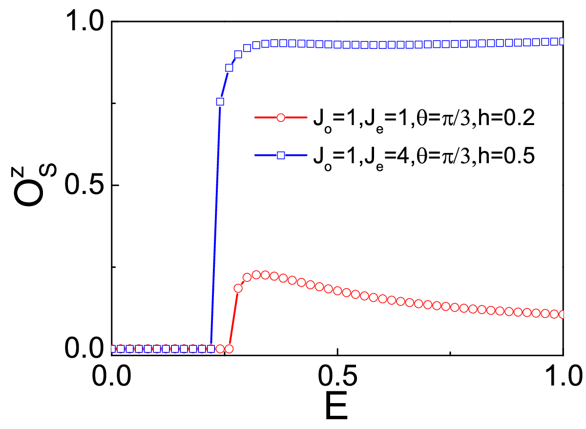
We adopt an infinite time-evolving block decimation (iTEBD) algorithm [34, 35], which allows one to solve for the ground state properties of a 1D translationally invariant spin system of infinite length. A crucial quantity during this strategy is the bond dimension , i.e., the cut-off dimension of Schmidt coefficients during singular value decomposition process. Figure 6 reveals that a nonlocal correlation arises in the both gapless and gapped chiral phases. The presence of a nonzero string order parameter indicates a hidden symmetry breaking through the Kramers-Wannier dual transformation [35], which can be related to a symmetry-protected topological order.


IV Thermodynamics
So far our study focuses on the ground state. In practice, we can only work at low but finite temperature, as close to absolute zero as possible, and the finite temperature properties is important theoretically and experimentally. Thanks to the exact solution of the GCM, it is straightforward to obtain its full thermodynamic properties at finite temperature. For the particle-hole excitation spectrum (35), the free energy of the quantum spin chain at temperature reads (here and below we use the units with the Boltzmann constant ),
| (41) |
Among many thermodynamic quantities, the entropy provides fundamental information about the evolution of spectra with increasing the temperature . The complete entropic landscape was recently quantitatively measured for Sr3Ru2O7 under magnetic field in the vicinity of quantum criticality [36]. It can be derived from the free energy (41) via the following thermodynamic relation,
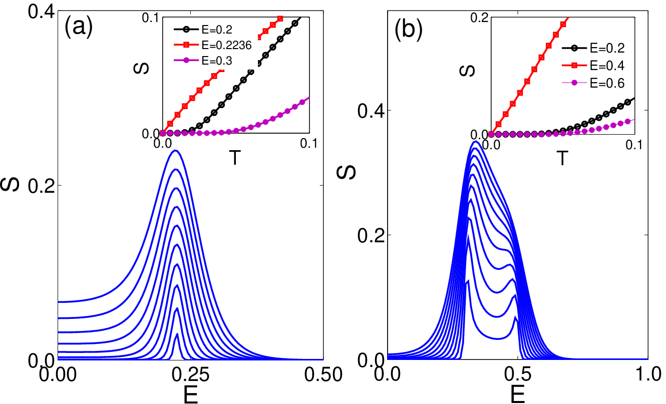
Figure 7 demonstrates the entropy as a function of the DM field and the temperature when the DM interaction is uniform. The entropy is vanishing asymptotically at zero temperature, and it grows with increasing when thermal excitations gradually include more and more excited states. One finds the entropy takes on a distinct maximum for increasing across a quantum critical point (QCP) at low temperature, annotating that the system is maximally undecided to select a state among the competing phases. The maximum get broader by increasing the temperature. The entropy shows an exponential activation with in the gaped phases, i.e., , as is indicated in insets of Fig.7. A scrutiny reveals that the entropy presents a linear dependence on , i.e., , for low temperatures in gapless phase, while at QCPs. This establishes a relation in the scaling theory to quantum criticality (here the spatial dimension is 1). This power-law dependence arises directly from the density of states in one dimension, . For the staggered DM interaction, the entropy in Fig.8 also exhibits local maxima across the QCPs. The entropy as a function of temperature also follows an identical scaling as Fig.7 as long as the Fermi-surface topology is guaranteed.

In addition, the low-temperature behavior of the heat capacity is readily measured, such as specific heat measurements of copper benzoate [37], transverse Ising magnet CoNb2O6 [38] and Heisenberg antiferromagneic Cu(C4H4N2)(NO3)2 [39]. Figure 9 shows a three-dimensional plot of the specific heat for =. The specific heat contains here a broad peak around the QCP and develops a local minimum at the top of the peak at the QCP for extremely low temperatures. By = , the specific heat also follows in gapless regimes, since is approximately proportional to . More precisely, at critical points [39]and in gapless chiral phase[38], in addition to an exponential activation in the gapped phases. Although the power-law scaling of the specific heat at the QCPs is identical to that of the entropy, the shallow trough in the specific heat implies that the critical temperature falls to zero as . A constant- contour measured at (see insets of Fig. 9) converges to a prominent peak profile for at the QCP, and the relatively high temperature quenches any discernible peak feature. For , two successive local minima show up in Fig.10, implying two QPTs with the increase of . The universal characteristic power laws in Tomonaga-Luttinger-liquid phase can be identified in the measured specific heat [39, 40].


V Conclusion
Plenteous intriguing phenomena in condensed matter systems originate from the interplay of strong interactions and frustrations. The dominating finite-range interactions in many-body systems can lead to kaleidoscopic self-ordered phases of matter. The one-dimensional generalized compass model mimics a distorted TM ion-oxygen ion-TM ion chain with a zigzag alignment, and it is one of very few quantum system to be exact solvable. In the paper, we study quantum phase transitions in this frustrated model as tuning an external magnetic field and staggered Dzyaloshinskii-Moriya interaction arising from the distortion. We present the exact solution by means of Jordan-Wigner transformation. We study the fermionic spectra, excitation gap, spin correlations, and critical properties at phase transitions. Then we establish the phase diagram. In order to uncover quantum critical behaviors of our model near the quantum critical points, we here supplement a temperature dependence of a few thermodynamic quantities, including entropy and specific heat. The entropy and specific heat exhibit characteristic power-law behavior with low temperature due to the density of states at Fermi surface, which is determined by low-energy excitations controlled by the dynamical exponent . at quantum critical point while in Tomonaga-Luttinger-liquid phase.
Acknowledgements.
We thank G.-H. Liu for helping us plot Fig.6. W.-L.Y. acknowledges support by the Natural Science Foundation of Jiangsu Province of China under Grant No. BK20141190 and the NSFC under Grant No. 11474211. W.-H. N. was financially supported by the NSFC under Grant No. 21473240.References
- [1] I. Dzyaloshinskii, J. Phys. Chem. Solids 4, 241 (1958).
- [2] T. Moriya, Phys. Rev. 120, 91 (1960).
- [3] A. Fert and P. M. Levy, Phys. Rev. Lett. 44, 1538 (1980).
- [4] S.-W. Cheong and M. Mostovoy, Nature Mater. 6, 13 (2007).
- [5] Hosho Katsura, Naoto Nagaosa, and Alexander V. Balatsky Phys. Rev. Lett. 95, 057205 (2005); M. Mostovoy, Phys. Rev. Lett. 96, 067601 (2006).
- [6] Y. Tokura and S. Seki, Adv. Mater. 22, 1554 (2010).
- [7] S. Heinze, K. von Bergmann, M. Menzel, J. Brede, A. Kubetzka, R. Wiesendanger, G. Bihlmayer, and S. Blügel, Nat. Phys. 7, 713 (2011).
- [8] C. Moreau-Luchaire et al., Nat. Nanotechnol. 11, 444 (2016).
- [9] O. Boulle et al., Nat. Nanotechnol. 11 , 449 (2016).
- [10] Wanjun Jiang, Pramey Upadhyaya, Wei Zhang, Guoqiang Yu, M. Benjamin Jungfleisch, Frank Y. Fradin, John E. Pearson, Yaroslav Tserkovnyak3, Kang L. Wang, Olle Heinonen, Suzanne G. E. te Velthuis, Axel Hoffmann, Science 349, 283 (2015).
- [11] M. Bode, M. Heide, K. von Bergmann, P. Ferriani, S. Heinze, G. Bihlmayer, A. Kubetzka, O. Pietzsch, S. Blügel, and R. Wiesendanger, Nature (London) 447, 190 (2007).
- [12] J.P. Goff, D.A. Tennant, S.E. Nagler, Phys. Rev. B 52, 15992 (1995).
- [13] R. Jafari, M. Kargarian, A. Langari, and M. Siahatgar Phys. Rev. B 78, 214414 (2008).
- [14] W.-L. You, G.-H. Liu, P. Horsch, and A. M. Oleś, Phys. Rev. B 90, 094413 (2014).
- [15] Guang-Hua Liu, Wen-Long You, Wei Li, Gang Su, J. Phys.: Condens. Matter 27, 165602 (2015).
- [16] I. Affleck, M. Oshikawa, Phys. Rev. B 60, 1038 (1999).
- [17] Masaki Oshikawa and Ian Affleck, Phys. Rev. Lett. 79, 2883 (1997).
- [18] J. Z. Zhao, X. Q. Wang, T. Xiang, Z. B. Su, and L. Yu Phys. Rev. Lett. 90, 207204 (2003).
- [19] V. E. Dmitrienko, E. N. Ovchinnikova, S. P. Collins,G. Nisbet, G. Beutier, Y. O. Kvashnin, V. V. Mazurenko, A. I. Lichtenstein and M. I. Katsnelson£¬ Nature Phys. 10, 202 (2014).
- [20] P. Schauß, J. Zeiher, T. Fukuhara, S. Hild, M. Cheneau, T. Macrì, T. Pohl, I. Bloch, C. Gross, Science 347, 1455 (2015).
- [21] W.-L. You, P. Horsch, and A. M. Oleś, Phys. Rev. B 89, 104425 (2014).
- [22] W.-L. You, Y.-C. Qiu, and A. M. Oleś, Phys. Rev. B 93, 214417 (2016).
- [23] Masahito Mochizuki, Nobuo Furukawa, and Naoto Nagaosa, Phys. Rev. Lett. 105, 037205 (2010); Phys. Rev. B 84, 144409 (2011).
- [24] Y.-C. Qiu, Q.-Q. Wu and W.-L. You, J. Phys.: Condens. Matter, 28, 496001(2016).
- [25] U. Schotte, A. Kelnberger, N. Stsser, J. Phys.: Condens. Matter 10, 6391 (1998).
- [26] E. Barouch and B. M. McCoy, Phys. Rev. A 2, 1075 (1970); 3, 786 (1971).
- [27] Y. Xiong and P. Tong, New J. Phys. 17, 013017 (2015);X. Wang, T. Liu, and Y. Xiong and P. Tong, Phys. Rev. A 92, 012116 (2015).
- [28] R. Jafari and Henrik Johannesson, Phys. Rev. Lett. 118, 015701 (2017).
- [29] A. Altland and M. R. Zirnbauer, Phys. Rev. B 55, 1142 (1997).
- [30] Ching-Kai Chiu, Jeffrey C.Y. Teo, Andreas P. Schnyder, and Shinsei Ryu, Rev. Mod. Phys. 88, 035005 (2016).
- [31] A. Yu. Kitaev, Phys.-Usp. (Suppl.) 44, 131 (2001).
- [32] P. Ghosh, J. D. Sau, S. Tewari, and S. Das Sarma, Phys. Rev. B 82, 184525 (2010).
- [33] I. A. Sergienko and E. Dagotto, Phys. Rev. B 73, 094434 (2006).
- [34] G. Vidal, Phys. Rev. Lett. 98, 070201 (2007); R. Orús and G. Vidal, Phys. Rev. B 78, 155117 (2008).
- [35] G.-H. Liu, Wei Li, W.-L. You, G. Su, and G.-S. Tian, Eur. Phys. J. B 86, 227 (2013); G.-H. Liu, Wei Li, W.-L. You, G.-S. Tian, and G. Su, Phys. Rev. B 85, 184422 (2012).
- [36] A. W. Rost, R. S. Perry, J.-F. Mercure, A. P. Mackenzie, and S. A. Grigera, Science 325, 1360 (2009).
- [37] D. C. Dender, P. R. Hammar, Daniel H. Reich, C. Broholm, and G. Aeppli, Phys. Rev. Lett. 79, 1750 (1997).
- [38] Tian Liang, S. M. Koohpayeh, J. W. Krizan, T. M. McQueen, R. J. Cava and N. P. Ong, Nature Commun. 6, 7611 (2015).
- [39] Y. Kono, T. Sakakibara, C.P. Aoyama, C. Hotta, M.M. Turnbull, C.P. Landee, and Y. Takano, Phys. Rev. Lett. 114, 037202 (2015).
- [40] T. Xiang, Phys. Rev. B 58, 9142 (1998).