跳到论文正文
W Papers独立论文阅读器 arXiv:1705.10370 论文正文 计算阅读时间 · 0%
引用这篇论文根据当前论文元数据生成,正式投稿前建议核对。


License: arXiv.org perpetual non-exclusive license
arXiv:1705.10370v1 [stat.ME] 29 May 2017

Covariate Assisted Variable Ranking

Zheng Tracy Ke??    Fan Yang

Consider a linear model y=X​β+zy=X\beta+z, z∼N⁡(0,σ2​In)z\sim N(0,\sigma^{2}I_{n}). The Gram matrix Θ=1n​X′​X\Theta=\frac{1}{n}X^{\prime}X is non-sparse, but it is approximately the sum of two components, a low-rank matrix and a sparse matrix, where neither component is known to us. We are interested in the Rare/Weak signal setting where all but a small fraction of the entries of β\beta are nonzero, and the nonzero entries are relatively small individually. The goal is to rank the variables in a way so as to maximize the area under the ROC curve.

We propose Factor-adjusted Covariate Assisted Ranking (FA-CAR) as a two-step approach to variable ranking. In the FA-step, we use PCA to reduce the linear model to a new one where the Gram matrix is approximately sparse. In the CAR-step, we rank variables by exploiting the local covariate structures.

FA-CAR is easy to use and computationally fast, and it is effective in resolving signal cancellation, a challenge we face in regression models. FA-CAR is related to the recent idea of Covariate Assisted Screening and Estimation (CASE), but two methods are for different goals and are thus very different.

We compare the ROC curve of FA-CAR with some other ranking ideas on numerical experiments, and show that FA-CAR has several advantages. Using a Rare/Weak signal model, we derive the convergence rate of the minimum sure-screening model size of FA-CAR. Our theoretical analysis contains several new ingredients, especially a new perturbation bound for PCA.

and

University of Chicago

1 Introduction

Consider the linear model in the p≫np\gg n setting:

y=X​β+z,X=[x1,⋯,xp]∈ℝn,p,z∼N⁡(0,σ2​In).y=X\beta+z,\qquad X=[x_{1},\cdots,x_{p}]\in\mathbb{R}^{n,p},\qquad z\sim N(0,\sigma^{2}I_{n}). (1.1)

We are interested in variable ranking, a problem related to variable selection but very different. Scientific experiments are constrained by budget and manpower, and it is often impossible to completely separate the signals from the noise. An alternative is then to identify a few most promising variables for follow-up lab experiments. This is where variable ranking comes in.

In this paper, we call a nonzero entry of β\beta a “signal” and a zero entry a “noise.” We are interested in the Rare/Weak signal regime:

  • •

    (Rare). All but a small fraction of the entries of β\beta are nonzero.

  • •

    (Weak). Individually, the nonzero entries are relatively small.

We assume the Gram matrix Θ=(1/n)​X′​X\Theta=(1/n)X^{\prime}X follows an approximate factor model (Chamberlain and Rothschild, 1983; Fan, Liao and Mincheva, 2011):

Θ=∑k=1Kλk​vk​vk′+G0,K≪min⁡{n,p},\Theta=\sum_{k=1}^{K}\lambda_{k}v_{k}v_{k}^{\prime}+G_{0},\qquad K\ll\min\{n,p\}, (1.2)

where G0G_{0} is positive definite and sparse (in the sense that each row has relatively few large entries, with all other entries relatively small), λ1,⋯,λK\lambda_{1},\cdots,\lambda_{K} are positive, and v1,⋯,vKv_{1},\cdots,v_{K} are mutually orthogonal unit-norm vectors.

Model (1.2) is popular in finance (Connor and Korajczyk, 1993), where the low-rank part represents a few risk factors and G0G_{0} is the covariance matrix of the (weakly-correlated) idiosyncratic noise. It is also useful in microarray analysis, where the low-rank part represents technical, environmental, demographic, or genetic factors (Leek and Storey, 2007).

Marginal Ranking (MR) is an approach that is especially popular in genomics and genetics (Jeffery, Higgins and Culhane, 2006; Liu, Li and Wong, 2002). Recall that X=[x1,x2,…,xp]X=[x_{1},x_{2},\ldots,x_{p}]. The method ranks variables according to the marginal regression coefficients |(xj,y)|/(xj,xj)|(x_{j},y)|/(x_{j},x_{j}), 1≤j≤p1\leq j\leq p, where (⋅,⋅)(\cdot,\cdot) denotes the inner product. Marginal ranking has advantages: (a) It directly provides an explicit ranking that is reasonable in many cases; (b) It is easy-to-use and computationally fast; (c) It does not need tuning parameters; (d) It has a relatively less stringent requirement on noise distributions and provides reasonable results even when the noise distribution is unknown or when the features/samples are correlated.

Penalized methods are well-known variable selection approaches (Tibshirani, 1996; Fan and Li, 2001; Zou, 2006). However, compared to MR, penalization approaches are different in all the above aspects: (a) Variable selection and variable ranking are two different goals, and penalization methods do not automatically provide an explicit ranking; (b) They are computationally slower, especially when (n,p)(n,p) are large; (c) They usually require tuning; (d) They require more stringent conditions on the noise distribution; particularly, their behavior deteriorates when the noise distribution is misspecified (Wu and Wu, 2016).

Our goal is to improve MR so that it works well in our setting. Despite many good aspects of MR, we recognize that it faces two challenges:

  • •

    The KK factors in Θ\Theta may have a dominant effect, and the ranking by MR is only reasonable when these factors are removed.

  • •

    MR faces the so-called challenge of “signal cancellation” (Wasserman and Roeder, 2009).

Note that

E[(xj,y)/(xj,xj)]=(xj,xj)−1∑k:βk≠0(xj,xk)βk.E[(x_{j},y)/(x_{j},x_{j})]=(x_{j},x_{j})^{-1}\sum_{k:\beta_{k}\neq 0}(x_{j},x_{k})\beta_{k}.

“Signal cancellation” means that due to correlations among xjx_{j}’s, signals may have a mutual canceling effects, and variable jj may receive a relatively low ranking even when βj\beta_{j} is top-ranked among β1,β2,…,βp\beta_{1},\beta_{2},\ldots,\beta_{p}.

To overcome the challenges, we propose FA-CAR as a two-stage ranking method. FA-CAR contains a Factor-Adjusting (FA) step, where we use PCA for factor removal and reduce the linear model to a new one where the Gram matrix is sparse. In the Covariate-Assisted Ranking (CAR) step, we rank variables using covariate structures. We recognize that “signal cancellation” is only severe when the predictors are heavily correlated, and so by exploiting the covariate structures, we can significantly alleviate the canceling effects. Our major contributions are

  • •

    (A new ranking method). FA-CAR is easy to use and computationally fast, and it is effective in resolving “signal cancellation.” The numerical comparison of ROC curves shows that our method has advantages over some existing ranking methods.

  • •

    (Rate of convergence). Using a Rare/Weak signal model, we derive the convergence rate of the minimum sure-screening model size of FA-CAR. The advantage of FA-CAR is validated by the theoretical results.

  • •

    (New technical tools). In our analysis, we develop some new technical tools. Particularly, the FA step requires sharp perturbation analysis of PCA (Section 2.3), which is new to the best of our knowledge.

  • •

    (Extensions to GLM). We extend FA-CAR to a variable ranking method for generalized linear models (GLM).

1.1 Two illustrating examples

It is instructive to use two simple examples to illustrate why FA and CAR are useful.

Example 1 (One-factor design). Consider a case where the Gram matrix

Θ=Ip+ωp​ξ​ξ′,ωp>0 is a parameter,\Theta=I_{p}+\omega_{p}\xi\xi^{\prime},\qquad\mbox{$\omega_{p}>0$ is a parameter},

where ξ=η/‖η‖\xi=\eta/\|\eta\| with η∼N⁡(0,In)\eta\sim N(0,I_{n}) and σ2=0\sigma^{2}=0 so there is no noise. We assume β\beta has ss nonzeros and each nonzero equals to τ\tau (τ>0\tau>0). Even in this simple setting, many methods do not perform well. Take MR for example. As long as wp≪pw_{p}\ll p, we have n−1​(xj,xj)≈1n^{-1}(x_{j},x_{j})\approx 1 and

|(xj,y)|/(xj,xj)∼|ωp⋅(ξ,β)​ξj+βj|.|(x_{j},y)|/(x_{j},x_{j})\sim|\omega_{p}\cdot(\xi,\beta)\xi_{j}+\beta_{j}|.

Since |(ξ,β)​ξj|=Op​(τ​s/p)|(\xi,\beta)\xi_{j}|=O_{p}(\tau\sqrt{s}/p), whenever wp​s/p≫1w_{p}\sqrt{s}/p\gg 1, the factor has a non-negligible effect: the ranking depends more on ξ\xi instead of β\beta, and many signal variables may receive lower rankings than the noise variables.

Seemingly, the problem can be fixed if we use a factor removal step. Consider the Singular Vector Decomposition (SVD) of the design matrix XX:

X=∑k=1nλk​uk​vk′≡λ1​u1​v1′+X~,where​v1=ξ​and​X~=∑k=2nλk​uk​vk′.X=\sum_{k=1}^{n}\lambda_{k}u_{k}v_{k}^{\prime}\equiv\lambda_{1}u_{1}v_{1}^{\prime}+\tilde{X},\qquad\mbox{where}\;v_{1}=\xi\;\mbox{and}\;\tilde{X}=\sum_{k=2}^{n}\lambda_{k}u_{k}v_{k}^{\prime}.

We have two ways to remove the factor ξ\xi: one is to project the columns of XX using the projection matrix Hu=In−u1​u1′H_{u}=I_{n}-u_{1}u_{1}^{\prime}, and the other one is to project the rows of XX using the projection matrix Hv=Ip−v1​v1′H_{v}=I_{p}-v_{1}v_{1}^{\prime}. However, while both projections produce the same matrix:

X~=Hu​X=X​Hv,\tilde{X}=H_{u}X=XH_{v},

only the first one reduces Model (1.1) to a new linear model with the same vector β\beta. In particular, letting y~=Hu​y\tilde{y}=H_{u}y and ϵ~=Hu​ϵ\tilde{\epsilon}=H_{u}\epsilon, we have

y~=X~​β+z~,where​z~∼N⁡(0,σ2​Hu)​and​n−1​X~′​X~=Hv=Ip−ξ​ξ′.\tilde{y}=\tilde{X}\beta+\tilde{z},\qquad\mbox{where}\;\tilde{z}\sim N(0,\sigma^{2}H_{u})\;\mbox{and}\;n^{-1}\tilde{X}^{\prime}\tilde{X}=H_{v}=I_{p}-\xi\xi^{\prime}.

Similarly, if we write X~=[x~1,x~2,…,x~p]\tilde{X}=[\tilde{x}_{1},\tilde{x}_{2},\ldots,\tilde{x}_{p}] and apply MR, then n−1​(x~j,x~j)≈1n^{-1}(\tilde{x}_{j},\tilde{x}_{j})\approx 1 and

|(y~,x~j)|/(x~j,x~j)∼|(ξ,β)​ξj+βj|,|(\tilde{y},\tilde{x}_{j})|/(\tilde{x}_{j},\tilde{x}_{j})\sim|(\xi,\beta)\xi_{j}+\beta_{j}|,

where |(ξ,β)​ξj|=Op​(τ​s/p)|(\xi,\beta)\xi_{j}|=O_{p}(\tau\sqrt{s}/p) and has a negligible effect on the ranking. We therefore have a successful ranking scheme if we first remove the factor and then apply MR (in this simple setting, the sparse component G0G_{0} in Θ\Theta is diagonal). This is the basic idea of the FA step, which can be conveniently extended to cases where we have more than 11 factors.

Example 2. (Block-wise diagonal design). Suppose pp is even and Θ\Theta is block-wise diagonal, where each diagonal block takes the form of

(1hh1),h∈(−1,1) is a parameter.\begin{pmatrix}1&h\\ h&1\end{pmatrix},\qquad\mbox{$h\in(-1,1)$ is a parameter}.

The parameter σ2=0\sigma^{2}=0 so there is no noise. The vector β\beta only has three nonzeros (but we don’t know either the number of signals, or the locations or strengths of them):

β1=τ,β2=β3=aτ,where τ>0 and a∈ℝ.\beta_{1}=\tau,\qquad\beta_{2}=\beta_{3}=a\tau,\qquad\mbox{where $\tau>0$ and $a\in\mathbb{R}$}.

In this simple setting, even there is no factors in Θ\Theta, MR still does not perform well. For example, by direct calculations,

β2=a​τ,β4=0,|(x2,y)|/(x2,x2)=|a−h|​τ,|(x4,y)|/(x4,x4)=|a​h|​τ.\beta_{2}=a\tau,\quad\beta_{4}=0,\quad|(x_{2},y)|/(x_{2},x_{2})=|a-h|\tau,\quad|(x_{4},y)|/(x_{4},x_{4})=|ah|\tau.

Therefore, we may face severe signal cancellation at location 22, and variable 22 (a signal variable) is ranked under variable 44 (a noise variable) when

|a​h|>|a−h|.|ah|>|a-h|.

We recognize that this problem can be resolved by exploiting local covariate structures. For each variable jj, let

𝒜j={ℐ1,ℐ2},ℐ1={j},ℐ2={j,j+1} for j odd and ℐ2={j−1,j} for j even.{\cal A}_{j}=\{{\cal I}_{1},{\cal I}_{2}\},\quad{\cal I}_{1}=\{j\},\;\;\mbox{${\cal I}_{2}=\{j,j+1\}$ for $j$ odd and ${\cal I}_{2}=\{j-1,j\}$ for $j$ even.}

Each element ℐ∈𝒜j{\cal I}\in{\cal A}_{j} is called a “neighborhood” of jj. For each ℐ∈𝒜j{\cal I}\in{\cal A}_{j}, we measure the “significance” of variable jj in ℐ{\cal I} by

Tj|ℐ=‖Pℐ​y‖2−‖Pℐ∖{j}​y‖2,T_{j|{\cal I}}=\|P_{{\cal I}}y\|^{2}-\|P_{{\cal I}\setminus\{j\}}y\|^{2},

where PℐP_{{\cal I}} is the projection from ℝn\mathbb{R}^{n} to the space spanned by {xj,j∈ℐ}\{x_{j},j\in{\cal I}\}. Neglecting the influence of all variables outside the set ℐ{\cal I}, Tj|ℐT_{j|{\cal I}} is the likelihood ratio for testing whether supp​(β)=ℐ\text{supp}(\beta)={\cal I} or supp​(β)=ℐ∖{j}\text{supp}(\beta)={\cal I}\setminus\{j\}. Take an odd jj for example, where ℐ1={j}{\cal I}_{1}=\{j\} and ℐ2={j,j+1}{\cal I}_{2}=\{j,j+1\}. By direct calculations,

Tj|ℐ1=n​(βj+h​βj+1)2,Tj|ℐ2=n⁡(1−h2)​βj2.T_{j|{\cal I}_{1}}=n(\beta_{j}+h\beta_{j+1})^{2},\qquad T_{j|{\cal I}_{2}}=n(1-h^{2})\beta_{j}^{2}.

When both variables jj and (j+1)(j+1) are signals, signal cancellation only affects Tj|ℐ1T_{j|{\cal I}_{1}} but not Tj|ℐ2T_{j|{\cal I}_{2}}, so the latter is preferred. When variable jj is a signal and variable (j+1)(j+1) is a noise, signal cancellation affects neither of them; since Tj|ℐ1=n​βj2≥Tj|ℐ2T_{j|{\cal I}_{1}}=n\beta_{j}^{2}\geq T_{j|{\cal I}_{2}} in this case, Tj|ℐ1T_{j|{\cal I}_{1}} is preferred. This motivates us to assess the significance of variable jj by combining these scores:

Tj∗=max⁡{Tj|ℐ:ℐ∈𝒜j}.T_{j}^{*}=\max\big\{T_{j|{\cal I}}:{\cal I}\in{\cal A}_{j}\big\}.

In the above example,

T2∗=n​max⁡{a2​(1−h2),(a−h)2}​τ2,T4∗=n​(a​h)2​τ2,T_{2}^{*}=n\max\bigl\{a^{2}(1-h^{2}),(a-h)^{2}\bigr\}\tau^{2},\qquad T_{4}^{*}=n(ah)^{2}\tau^{2},

and variables 22 and 44 are ranked correctly as long as |h|<1/2≈0.7|h|<1/\sqrt{2}\approx 0.7.

In more general cases, we use Θ\Theta to construct a graph and let a “neighborhood” of jj be a connected subgraph that contains jj, and the above idea can thus be conveniently extended. This is the main idea of the CAR step.

Remark. It is possible to measure the significance differently by adding a cleaning step as in Ke, Jin and Fan (2014), and hopefully we can evaluate variable 44 with a score of 00. However, cleaning usually requires a few tuning parameters, which is the first thing we wish to avoid in variable ranking.

Remark. It is also possible to use the coefficients of a penalized-regression estimator (e.g., the lasso) for ranking. Such estimators still require a critical tuning parameter that we wish to avoid. Additionally, when noise presents (σ2≠0\sigma^{2}\neq 0), these methods are less effective than screening methods for the blockwise-diagonal design; see Jin, Zhang and Zhang (2014) and Section 1.4.

1.2 Factor-adjusted Covariate Assisted Ranking (FA-CAR)

We extend the intuition gained in illustrating examples and develop a ranking method that works for a general design from Model (1.2). The method consists of a Factor-Adjusting (FA) step and a Covariate Assisted Ranking (CAR) step.

In the FA step, let X=∑k=1nσ^k​u^k​v^k′X=\sum_{k=1}^{n}\hat{\sigma}_{k}\hat{u}_{k}\hat{v}_{k}^{\prime} be the SVD of XX, where σ^1≥σ^2≥⋯≥σ^n>0\hat{\sigma}_{1}\geq\hat{\sigma}_{2}\geq\cdots\geq\hat{\sigma}_{n}>0 are the singular values, and u^k∈ℝn\hat{u}_{k}\in\mathbb{R}^{n} and v^k∈ℝp\hat{v}_{k}\in\mathbb{R}^{p} are the kk-th (unit-norm) left and right singular vectors, respectively. Introduce

y~=y−∑k=1K(u^k′​y)​u^k,X~=X−∑k=1Kσ^k​u^k​v^k′.\tilde{y}=y-\sum_{k=1}^{K}(\hat{u}_{k}^{\prime}y)\hat{u}_{k},\qquad\tilde{X}=X-\sum_{k=1}^{K}\hat{\sigma}_{k}\hat{u}_{k}\hat{v}_{k}^{\prime}. (1.3)

If we consider the two projection matrices Hu=In−∑k=1Ku^k​u^k′H_{u}=I_{n}-\sum_{k=1}^{K}\hat{u}_{k}\hat{u}_{k}^{\prime} and Hv=Ip−∑k=1Kv^k​v^k′H_{v}=I_{p}-\sum_{k=1}^{K}\hat{v}_{k}\hat{v}_{k}^{\prime}, then it follows from elementary linear algebra that y~=Hu​y\tilde{y}=H_{u}y, X~=Hu​X=X​Hv\tilde{X}=H_{u}X=XH_{v}, and (1/n)​X~′​X~=Hv​Θ​Hv(1/n)\tilde{X}^{\prime}\tilde{X}=H_{v}\Theta H_{v}. As a result,

y~=X~​β+z~,where ​z~∼N⁡(0,σ2​Hu)​ and ​n−1​X~′​X~=Θ−∑k=1K(σ^k2/n)​v^k​v^k′.\tilde{y}=\tilde{X}\beta+\tilde{z},\quad\mbox{where }\tilde{z}\sim N(0,\sigma^{2}H_{u})\mbox{ and }n^{-1}\tilde{X}^{\prime}\tilde{X}=\Theta-\sum_{k=1}^{K}(\hat{\sigma}_{k}^{2}/n)\hat{v}_{k}\hat{v}_{k}^{\prime}. (1.4)

This gives a new linear model with the same β\beta but a different Gram matrix. Note that (σ^k2/n)(\hat{\sigma}_{k}^{2}/n) and v^k\hat{v}_{k} are the kk-th eigenvalue and eigenvector of Θ\Theta, respectively. In Model (1.2), the component G0G_{0} is a sparse matrix. Therefore, the leading eigenvalues (eigenvectors) of Θ\Theta are approximately equal to the leading eigenvalues (eigenvectors) of (Θ−G0)(\Theta-G_{0}), i.e., (σ^k2/n)≈λk(\hat{\sigma}_{k}^{2}/n)\approx\lambda_{k} and v^k≈vk\hat{v}_{k}\approx v_{k} for 1≤k≤K1\leq k\leq K. We thus have

(1/n)​X~′​X~≈Θ−∑k=1Kλk​vk​vk′=G0.(1/n)\tilde{X}^{\prime}\tilde{X}\approx\Theta-\sum_{k=1}^{K}\lambda_{k}v_{k}v_{k}^{\prime}=G_{0}.

So the Gram matrix for Model (1.4) is sparse.

In the CAR step, we focus on Model (1.4). Write X~=[x~1,…,x~p]\tilde{X}=[\tilde{x}_{1},\ldots,\tilde{x}_{p}] and G=(1/n)​X~′​X~G=(1/n)\tilde{X}^{\prime}\tilde{X}. Given a threshold δ∈(0,1)\delta\in(0,1), let 𝒢δ{\cal G}^{\delta} be the graph with nodes {1,2,…,n}\{1,2,\ldots,n\} such that nodes ii and jj are connected by an undirected edge if

|G⁡(i,j)|/G⁡(i,i)​G​(j,j)>δ,1≤i≠j≤p.|G(i,j)|/\sqrt{G(i,i)G(j,j)}>\delta,\qquad 1\leq i\neq j\leq p. (1.5)

For each variable jj, any connected subgraph ℐ{\cal I} of 𝒢δ{\cal G}^{\delta} that contains jj is called a “neighborhood” of jj. Consider a collection of such local “neighborhoods”

𝒜δ,j(m)={ℐ is a connected subgraph of 𝒢δ:j∈ℐ,|ℐ|≤m},{\cal A}_{\delta,j}(m)=\big\{\mbox{${\cal I}$ is a connected subgraph of ${\cal G}^{\delta}$}:j\in{\cal I},\;|{\cal I}|\leq m\big\}, (1.6)

where m≥1m\geq 1 is an integer that controls the maximum size of selected neighborhoods. For ℐ∈𝒜δ,j​(m){\cal I}\in{\cal A}_{\delta,j}(m), we measure the “significance” of variable jj in ℐ{\cal I} by

Tj|ℐ=‖Pℐ​y~‖2−‖Pℐ∖{j}​y~‖2,T_{j|{\cal I}}=\|P_{{\cal I}}\tilde{y}\|^{2}-\|P_{{\cal I}\setminus\{j\}}\tilde{y}\|^{2}, (1.7)

where Pℐ​y~P_{{\cal I}}\tilde{y} is the projection of y~\tilde{y} onto the space spanned by {x~j:j∈ℐ}\{\tilde{x}_{j}:j\in{\cal I}\}. We then measure the “significance” of variable jj by combining these scores:

Tj∗=max⁡{Tj|ℐ:ℐ∈𝒜δ,j​(m)}.T_{j}^{*}=\max\big\{T_{j|{\cal I}}:{\cal I}\in{\cal A}_{\delta,j}(m)\big\}. (1.8)

The scores T1∗,T2∗,…,Tp∗T_{1}^{*},T_{2}^{*},\ldots,T_{p}^{*} are used to rank variables.

FA-CAR has tuning parameters (m,K,δ)(m,K,\delta), but the ideal choice of tuning parameters is insensitive to the unknown β\beta (it mainly depends on the design XX). Therefore, tuning here is not as critical as it is for variable selection. In practice, we recommend using m=2m=2 and δ=0.5\delta=0.5 and choosing KK as the elbow point in the scree plot of the Gram matrix Θ\Theta (see Section 3).

The computational cost of our method comes from two parts: the SVD on XX and the CAR step. SVD is a rather manageable algorithm even for large matrices (Halko, Martinsson and Tropp, 2011). The computational cost of the CAR step is determined by the total number of subsets in the collection 𝒜δ(m)≡∪j=1p𝒜δ,j(m){\cal A}_{\delta}(m)\equiv\cup_{j=1}^{p}{\cal A}_{\delta,j}(m). By graph theory (Frieze and Molloy, 1999),

|𝒜δ(m)|≤pm(2.72dp)m,dp: maximum node degree.|{\cal A}_{\delta}(m)|\leq pm(2.72d_{p})^{m},\qquad\mbox{$d_{p}$: maximum node degree}.

Since G≈G0G\approx G_{0} is sparse, dpd_{p} grows slowly with pp. So the computational cost of the CAR step is only moderately larger than that of MR.

Our method can also be conveniently extended to generalized linear models (GLM), which we discuss in Section 4.

1.3 Application to a microarray dataset

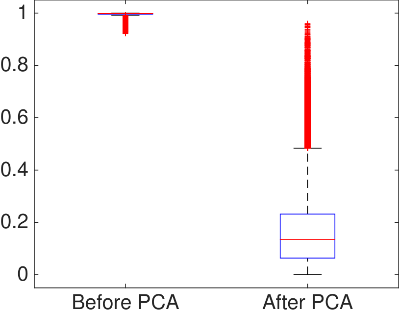
We investigate the performance of our method using a gene microarray dataset (Nayak et al., 2009). It contains the gene expressions of human immortalized B cells for p=4238p=4238 genes and n=148n=148 subjects (CEPH-Utah subpopulation). We use this n×pn\times p data matrix as the design. Figure 1 compares the two respective Gram matrices for Model (1.1) and Model (1.4), and it shows that the Gram matrix for Model (1.4) is much sparser. This suggests that our assumption (1.2) fits the data well and that the FA step is effective in removing the factors.

We then compare our method with three other ranking methods on synthetic experiments. MR uses marginal correlation coefficients to rank variables. HOLP (Wang and Leng, 2015) and RRCS (Li et al., 2012) are variants of MR: HOLP uses the absolute coordinates of X′​(X​X′)−1​yX^{\prime}(XX^{\prime})^{-1}y to rank variables, and RRSC uses the Kendall’s τ\tau marginal correlation coefficients. We measure the ranking performance using the Receiver Operating Characteristic (ROC) curve: Given the rank of variables, the ROC curve is obtained by successively retaining more variables.

In our experiment, fixing parameters (η,s)(\eta,s), we first generate β\beta by drawing its first ss coordinates i​i​diid from N⁡(0,η2)N(0,\eta^{2}) and setting the other coordinates to be 00 and then generate yy using Model (1.1) with σ=1\sigma=1. Here, (η,s)(\eta,s) control the signal strength and signal sparsity, respectively. For each method, we report the average ROC curves over 200200 repetitions; the results are displayed in Figure 2. When s=50s=50, FA-CAR always yields the best performance, and it is especially advantageous when η\eta is small (i.e., the signals are “weak”). When s=10s=10, FA-CAR performs reasonably well, and it is better than MR. It is a little worse than HOLP and RRSC, but these two methods are unsatisfactory in the other settings. In terms of the overall performance, we conclude that FA-CAR is the best among the four methods.

Refer to caption
Refer to caption
Refer to caption
Fig 1: Left two panels: the Gram matrix before and after Factor Adjusting (for presentation purpose, both matrices have been normalized so that the diagonals are 11; only the upper left 100×100100\times 100 block is displayed). Right panel: Boxplots of the off-diagonal entries (in absolute value) of two Gram matrices.
Fig 2: The ROC. Design: gene-microarray. The curves are averaged over 200200 repetitions.

1.4 Comparison of the sure-screening model size

We use the blockwise-diagonal example in Section 1.1 to demonstrate the advantage of exploiting local covariate structures for ranking. We use the sure-screening model size as the loss function, which is the minimum number of top-ranked variables one needs to select such that all signals are retained (then, all signal variables will be included in the follow-up lab experiments, say).

We adopt a Rare/Weak (RW) signal model, which has been used a lot in the literature (Donoho and Jin, 2004; Ji and Jin, 2012). Fixing ϑ∈(0,1)\vartheta\in(0,1) and r>0r>0, we assume the vector β\beta is generated from (νa\nu_{a}: a point mass at aa)

βj​∼i​i​d​(1−ϵp)​ν0+ϵp2​ντp+ϵp2​ν−τp,ϵp=p−ϑ,τp=σ​2​r​log⁡(p)/n.\beta_{j}\overset{iid}{\sim}(1-\epsilon_{p})\nu_{0}+\frac{\epsilon_{p}}{2}\nu_{\tau_{p}}+\frac{\epsilon_{p}}{2}\nu_{-\tau_{p}},\quad\epsilon_{p}=p^{-\vartheta},\tau_{p}=\sigma\sqrt{2r\log(p)/n}. (1.9)

Under (1.9), the total number of signals is approximately sp≡p1−ϑs_{p}\equiv p^{1-\vartheta}; as pp grows, the signals become increasingly sparser. The two parameters (ϑ,r)(\vartheta,r) characterize the signal rareness and signal weakness, respectively. For any threshold t>0t>0, let F​Np​(t)=∑j=1pℙ⁡(βj≠0,Tj∗≤t)FN_{p}(t)=\sum_{j=1}^{p}\mathbb{P}(\beta_{j}\neq 0,T_{j}^{*}\leq t) and F​Pp​(t)=∑j=1pℙ⁡(βj=0,Tj∗>t)FP_{p}(t)=\sum_{j=1}^{p}\mathbb{P}(\beta_{j}=0,T_{j}^{*}>t) be the expected number of false negative and false positives, respectively. Define the sure-screening model size as

SSp∗(ϑ,r,h)=sp+mint:F​Np​(t)<1FPp(t).SS^{*}_{p}(\vartheta,r,h)=s_{p}+\min_{t:FN_{p}(t)<1}FP_{p}(t).

For the blockwise diagonal design, the Gram matrix is already sparse, so the FA step is not needed. We compare CAR with two other ideas, MR and LSR, where LSR simultaneously runs least-squares on each pair of variables {2​j−1,2​j}\{2j-1,2j\} for j=1,2,…,p/2j=1,2,\ldots,p/2 and uses these least-squares coefficients to rank variables. We note that the least-squares estimator coincides with the recent de-biased lasso estimator (Zhang and Zhang, 2014; van de Geer et al., 2014) in this design. The following lemma shows that the convergence rate of S​Sp∗​(ϑ,r,h)SS_{p}^{*}(\vartheta,r,h) for CAR is always no slower than those of the other two methods.

Lemma 1 (Sure-screening model size).

Consider Model (1.1) with the blockwise-diagonal design as in Section 1.1, where the RW model (1.9) holds. Let LpL_{p} denote a generic multi-log⁡(p)\log(p) term such that Lp​p−δ→0L_{p}p^{-\delta}\to 0 and Lp​pδ→∞L_{p}p^{\delta}\to\infty for all δ>0\delta>0. Given any (ϑ,r,h)∈(0,1)×(0,∞)×(−1,1)(\vartheta,r,h)\in(0,1)\times(0,\infty)\times(-1,1), for each of the three methods, there is a constant η∗​(ϑ,r,h)∈[0,1]\eta^{*}(\vartheta,r,h)\in[0,1] such that S​Sp∗​(ϑ,r,h)=Lp​pη∗​(ϑ,r,h)SS^{*}_{p}(\vartheta,r,h)=L_{p}p^{\eta^{*}(\vartheta,r,h)}. Furthermore, for all (ϑ,r,h)(\vartheta,r,h),

ηC​A​R∗​(ϑ,r,h)≤min⁡{ηM​R∗​(ϑ,r,h),ηL​S​R∗​(ϑ,r,h)}.\eta^{*}_{CAR}(\vartheta,r,h)\leq\min\big\{\eta^{*}_{MR}(\vartheta,r,h),\;\;\eta^{*}_{LSR}(\vartheta,r,h)\bigr\}.

The explicit expression of η∗​(ϑ,r,h)\eta^{*}(\vartheta,r,h) for all three methods can be found in Lemma 6. Using the results there, we can find settings where the convergence rate of CAR is strictly faster; see Table 1.

Table 1: The exponent η∗​(ϑ,r,h)\eta^{*}(\vartheta,r,h) for the blockwise-diagonal design.
(ϑ,r,|h|)(\vartheta,r,|h|) (.8,1.5,.4)(.8,1.5,.4) (.5,2,.8)(.5,2,.8) (.3,2,.2)(.3,2,.2)
CAR .395 .500 .700
MR .395 .920 .751
LSR .543 .980 .700

Remark. One might wonder why LSR is not the best method for ranking. This is a consequence of signal sparsity. When the signals are sparse, most of the 22-by-22 blocks that contain signals have exactly one signal, so the least squares estimator is less efficient than the marginal estimator for estimating a signal βj\beta_{j}.

1.5 Connections

Our method is related to the recent ideas of Graphlet Screening (GS) (Jin, Zhang and Zhang, 2014) and Covariate Assisted Screening and Estimation (CASE) (Ke, Jin and Fan, 2014). These methods also use Θ\Theta to construct a graph and use local graphical structures to improve inference. However, our settings and goals are very different, and our method/theory can not be deduced from previous works: (a) GS and CASE are for variable selection and it is unclear how to use them for variable ranking. (b) GS and CASE have more stringent assumptions on the Gram matrix and do not work for the general designs considered in this paper.

Our FA step is related to the idea of using PCA to remove factor structures in multiple testing (Fan, Han and Gu, 2012) and covariance estimation (Fan, Liao and Mincheva, 2013), but our FA step is designed for linear models and is thus very different. Wang (2012) used PCA to improve marginal screening, which is similar to our FA step; however, their PCA approach is only justified for a random design that comes from an exact factor model, and their theory is insufficient for justifying our FA step.

Our work is related to the literatures on ranking differently expressed genes (Chen et al., 2007). Common gene-ranking approaches (e.g., pp-value, fold-change) are connected to the idea of Marginal Ranking. The key idea of our method is to exploit correlation structures among variables to improve MR, and an extension of our method (Section 4) can be potentially used for gene-ranking. On a high level, our work is also related to feature ranking problem in machine learning (Guyon and Elisseeff, 2003), but most methods in these literatures (e.g., wrappers, filters) are algorithm-based and are not designed specifically for linear models.

1.6 Content and notations

The remaining of this paper is organized as follows. Section 2 contains asymptotic analysis, and Section 3 contains numerical results. Section 4 provides an extension to generalized linear models. The discussions are in Section 5. Proofs are relegated to Section 6.

Throughout this paper, For positive sequences {an}n=1∞\{a_{n}\}_{n=1}^{\infty} and {bn}n=1∞\{b_{n}\}_{n=1}^{\infty}, we write an=o⁡(bn)a_{n}=o(b_{n}), an=O⁡(bn)a_{n}=O(b_{n}) and an≲bna_{n}\lesssim b_{n}, if limn→∞(an/bn)=0\lim_{n\to\infty}(a_{n}/b_{n})=0, limsupn→∞(an/bn)<∞\lim\sup_{n\to\infty}(a_{n}/b_{n})<\infty, max⁡{an−bn,0}=o⁡(1)\max\{a_{n}-b_{n},0\}=o(1), respectively. Given 0≤q≤∞0\leq q\leq\infty, for any vector xx, ‖x‖q\|x\|_{q} denotes the LqL_{q}-norm of xx; for any m×nm\times n matrix AA, ‖A‖q\|A\|_{q} denotes the matrix LqL_{q}-norm of AA; when q=2q=2, it coincides with the the spectral norm, and we omit the subscript qq. ‖A‖F\|A\|_{F} denotes the Frobenius norm and ‖A‖max\|A\|_{\max} denotes the entrywise max norm. When AA is symmetric, λmax​(A)\lambda_{\max}(A) and λmin​(A)\lambda_{\min}(A) denote the maximum and minimum eigenvalues, respectively. For two sets ℐ⊂{1,2,…,m}{\cal I}\subset\{1,2,\dots,m\} and 𝒥⊂{1,2,…,n}{\cal J}\subset\{1,2,\dots,n\}, Aℐ,𝒥A^{{\cal I},{\cal J}} denotes the submatrix of AA formed by restricting the rows and columns of AA to sets ℐ{\cal I} and 𝒥{\cal J}. For a vector x∈ℝpx\in\mathbb{R}^{p} and set ℐ⊂{1,2,…,p}{\cal I}\subset\{1,2,\dots,p\}, xℐx^{{\cal I}} denotes the sub-vector of xx formed by restricting coordinates to set ℐ{\cal I}.

2 Asymptotic analysis

We describe the asymptotic settings in Section 2.1 and present the main results in Section 2.2; our main results contain the rate of convergence of the sure-screening model size. Section 2.3 contains some new perturbation bounds for PCA; they are the key for studying Factor Adjusting and are also useful technical tools for other problems. Section 2.4 contains the proof of the main result.

2.1 Assumptions

We assume Θ\Theta has unit diagonals without loss of generality. Let SS be the support of β\beta and let sp=|S|s_{p}=|S|. We assume

log(p)/n→0,sp≤p1−ϑfor some ϑ∈(0,1).\log(p)/n\rightarrow 0,\qquad s_{p}\leq p^{1-\vartheta}\quad\mbox{for some $\vartheta\in(0,1)$.} (2.1)

Under (2.1), it is known that n−1/2log⁡(p)n^{-1/2}\sqrt{\log(p)} is the minimax order of signal strength for successful variable selection (Ji and Jin, 2012). We focus on the most subtle region that nonzero βj\beta_{j}’s are constant multiples of n−1/2log⁡(p)n^{-1/2}\sqrt{\log(p)}. Fixing a constant r>0r>0 that calibrates the signal strength and a constant a>0a>0, we assume for any j∈Sj\in S,

τp≤|βj|≤aτp,whereτp=n−1/2σ2​r​log⁡(p).\tau_{p}\leq|\beta_{j}|\leq a\tau_{p},\qquad\mbox{where}\quad\tau_{p}=n^{-1/2}\sigma\sqrt{2r\log(p)}. (2.2)

Model (2.1)-(2.2) is a non-stochastic version of the Rare/Weak signal model in the literatures (Jin and Ke, 2016).

The Gram matrix Θ\Theta satisfies model (1.2). For any integer 1≤m≤p1\leq m\leq p and matrix Ω∈ℝp,p\Omega\in\mathbb{R}^{p,p}, define νm∗​(Ω)\nu_{m}^{\ast}(\Omega) as the minimum possible eigenvalue of any m×mm\times m principal submatrix of Ω\Omega. Fixing γ∈(0,1)\gamma\in(0,1), c0,C0>0c_{0},C_{0}>0 and an integer g≥1g\geq 1, we introduce a class of sparse covariance matrices:

ℳp(g,γ,c0,C0)={Ω∈ℝp,p is p.s.d.:νg∗(Ω)≥c0,max1≤i≤p∑j=1p|Ω(i,j)|γ≤C0}.{\cal M}_{p}(g,\gamma,c_{0},C_{0})=\Big\{\Omega\in\mathbb{R}^{p,p}\mbox{ is p.s.d.}:\nu_{g}^{\ast}(\Omega)\geq c_{0},\;\max_{1\leq i\leq p}\sum_{j=1}^{p}|\Omega(i,j)|^{\gamma}\leq C_{0}\Big\}.

Recall that G0G_{0} is the sparse component in Model (1.2). We assume

G0∈ℳp​(g,γ,c0,C0),λ1≤c1​λK,λK/max⁡{sp,log⁡(p)}→∞,G_{0}\in{\cal M}_{p}(g,\gamma,c_{0},C_{0}),\quad\lambda_{1}\leq c_{1}\lambda_{K},\quad\lambda_{K}/\max\{s_{p},\log(p)\}\rightarrow\infty, (2.3)

where c1>0c_{1}>0 is a constant. Fixing a constant b>0b>0, let 𝒢0δ{\cal G}_{0}^{\delta} be the undirected graph whose nodes are {1,⋯,p}\{1,\cdots,p\} and there is an edge between nodes ii and jj if and only if

|G0​(i,j)|/G0​(i,i)​G0​(j,j)>δp,whereδp=b/log⁡(p).|G_{0}(i,j)|/\sqrt{G_{0}(i,i)G_{0}(j,j)}>\delta_{p},\qquad\mbox{where}\quad\delta_{p}=b/\log(p).

This graph can be viewed as the “oracle” graph, and the graph 𝒢δ{\cal G}^{\delta} used in our method is an approximation to 𝒢0δ{\cal G}_{0}^{\delta}. Let 𝒢0,Sδ{\cal G}_{0,S}^{\delta} be the induced graph by restricting nodes to SS. We assume that for a positive integer ℓ0≤g\ell_{0}\leq g,

each component of 𝒢0,Sδ consists of ≤ℓ0 nodes.\mbox{each component of ${\cal G}_{0,S}^{\delta}$ consists of $\leq\ell_{0}$ nodes}. (2.4)

This is an assumption on the correlation structures among signal variables. It implies that the signal variables divide into many groups, each consisting of ≤ℓ0\leq\ell_{0} variables, such that signals in distinct groups are only weakly correlated after the factors are removed.

FA-CAR has tuning parameters (K,m,δ)(K,m,\delta). We choose KK adaptively by

K=K^p=max⁡{1≤k≤n:σ^k2>n​log⁡(p)},K=\hat{K}_{p}=\max\big\{1\leq k\leq n:\hat{\sigma}^{2}_{k}>n\log(p)\big\}, (2.5)

where σ^k\hat{\sigma}_{k} is the kk-th leading singular value of XX. We choose (m,δ)(m,\delta) such that, for some constant C>0C>0,

ℓ0≤m≤g,1.01​δp≤δ≤C​δp,\ell_{0}\leq m\leq g,\qquad 1.01\delta_{p}\leq\delta\leq C\delta_{p}, (2.6)

where δp=b/log⁡(p)\delta_{p}=b/\log(p), gg and ℓ0\ell_{0} are defined in (2.3) and (2.4) respectively.

2.2 Main result: Sure-screening model size

Given the scores T1∗,…,Tp∗T_{1}^{*},\ldots,T_{p}^{*}, if we threshold them by

tp​(q)=2​q​σ2​log⁡(p),q>0 is a constant,t_{p}(q)=2q\sigma^{2}\log(p),\qquad\mbox{$q>0$ is a constant}, (2.7)

the set of retained variables is S^​(q)=S^p​(q,X,y)={1≤j≤p:Tj∗>tp​(q)}\hat{S}(q)=\hat{S}_{p}(q;X,y)=\{1\leq j\leq p:T^{*}_{j}>t_{p}(q)\}. Recall that SS is the support of β\beta and sp=|S|s_{p}=|S|. The (asymptotic) sure-screening model size is defined as

S​Sp∗​(ϑ,r,X,β)=sp+min⁡{𝔼⁡(|S^​(q)∖S|):q satisfies​limp→∞𝔼⁡(|S∖S^​(q)|)=0}.SS^{*}_{p}(\vartheta,r;X,\beta)=s_{p}+\min\Bigl\{\mathbb{E}(|\hat{S}(q)\setminus S|):\mbox{$q$ satisfies}\lim_{p\to\infty}\mathbb{E}(|S\setminus\hat{S}(q)|)=0\Bigr\}. (2.8)

To describe the asymptotic behavior of S​Sp∗SS_{p}^{*}, we introduce the quantities ωj​(r,m)\omega_{j}(r,m), 1≤j≤p1\leq j\leq p, where rr calibrates the signal strength and m≥1m\geq 1 is a parameter in FA-CAR. By assumption (2.4), the set of signal variables SS has the decomposition S=ℐ1∪ℐ2∪…∪ℐMS={\cal I}_{1}\cup{\cal I}_{2}\cup\ldots\cup{\cal I}_{M}, where nodes in each ℐk{\cal I}_{k} form a component of 𝒢0,Sδ{\cal G}^{\delta}_{0,S} and max1≤k≤M⁡|ℐk|≤ℓ0\max_{1\leq k\leq M}|{\cal I}_{k}|\leq\ell_{0}. Fix jj. There exists a unique ℐk{\cal I}_{k} which contains jj. For any ℐ⊂ℐk{\cal I}\subset{\cal I}_{k}, let N=ℐ∖{j}N={\cal I}\setminus\{j\}, F=ℐk∖ℐF={\cal I}_{k}\setminus{\cal I}, and Aj|ℐ0=G0j,j−G0j,N​(G0N,N)−1​G0N,jA_{j|{\cal I}}^{0}=G_{0}^{j,j}-G_{0}^{j,N}(G_{0}^{N,N})^{-1}G_{0}^{N,j}. Define

ωj|ℐ​(r,G0,β,δp)=n​Aj|ℐ02​σ2​log⁡(p)​{βj+(Aj|ℐ0)−1​[G0j,F−G0j,N​(G0N,N)−1​G0N,F]​βF}2.\omega_{j|{\cal I}}(r;G_{0},\beta,\delta_{p})=\frac{nA_{j|{\cal I}}^{0}}{2\sigma^{2}\log(p)}\left\{\beta_{j}+(A_{j|{\cal I}}^{0})^{-1}[G_{0}^{j,F}-G_{0}^{j,N}(G_{0}^{N,N})^{-1}G_{0}^{N,F}]\beta^{F}\right\}^{2}. (2.9)

For each m≥1m\geq 1, define

ωj(r,m;G0,β,δp)=max{ωj|ℐ(r;G0,β,δp):ℐ∈𝒜δ,j(m),ℐ⊂ℐk}.\omega_{j}(r,m;G_{0},\beta,\delta_{p})=\max\left\{\omega_{j|{\cal I}}(r;G_{0},\beta,\delta_{p}):{\cal I}\in{\cal A}_{\delta,j}(m),{\cal I}\subset{\cal I}_{k}\right\}. (2.10)

We notice that ωj​(r,m)\omega_{j}(r,m) is a monotone increasing function of mm. The following definition is useful:

Definition 1.

LpL_{p}, as a positive sequence indexed by pp, is called a multi-log⁡(p)\log(p) term if for any fixed c>0c>0, Lp​pc→∞L_{p}p^{c}\rightarrow\infty and Lp​p−c→0L_{p}p^{-c}\rightarrow 0 as p→∞p\rightarrow\infty.

The following theorem gives an upper bound for rate of convergence

Theorem 1 (Sure-screening model size).

Under Model (1.1)-(1.2), suppose (2.1)-(2.4) hold for fixed (ϑ,r,g,ℓ0,γ,c0,C0,c1,a,b)(\vartheta,r,g,\ell_{0},\gamma,c_{0},C_{0},c_{1},a,b) such that g≥ℓ0g\geq\ell_{0}, and suppose the tuning parameters (K,m,δ)(K,m,\delta) satisfy (2.5)-(2.6). Define the constant

q∗​(ϑ,r,m,G0,β,δp)=inf{q≥0:lim¯p→∞⁡log⁡(∑j∈Sp−[(ωj​(r,m)−q)+]2)log⁡(p)>0}.q^{*}(\vartheta,r,m;G_{0},\beta,\delta_{p})=\inf\left\{q\geq 0:\mathop{\overline{\rm lim}}_{p\to\infty}\frac{\log\Big(\sum_{j\in S}p^{-[(\sqrt{\omega_{j}(r,m)}-\sqrt{q})_{+}]^{2}}\Big)}{\log(p)}>0\right\}.

Then, as p→∞p\rightarrow\infty,

S​Sp∗​(ϑ,r,X,β)≤Lp​p1−min⁡{ϑ,q∗​(ϑ,r,m)}.SS_{p}^{*}(\vartheta,r;X,\beta)\leq L_{p}p^{1-\min\{\vartheta,\;q^{*}(\vartheta,r,m)\}}.

We use Theorem 1 to draw some conclusions. First, we introduce a lower bound for the quantities ωj​(r,m)\omega_{j}(r,m). Fix jj and let ℐk{\cal I}_{k} be the component of 𝒢0,Sδ{\cal G}^{\delta}_{0,S} that contains jj. Write N=ℐk∖{j}N={\cal I}_{k}\setminus\{j\} and Aj|ℐk0=G0j,j−G0j,N​(G0N,N)−1​G0N,jA_{j|{\cal I}_{k}}^{0}=G_{0}^{j,j}-G_{0}^{j,N}(G_{0}^{N,N})^{-1}G_{0}^{N,j}. Define

ωj∗​(r,G0,β,δp)=n​Aj|ℐk02​σ2​log⁡(p)​βj2.\omega^{*}_{j}(r;G_{0},\beta,\delta_{p})=\frac{nA_{j|{\cal I}_{k}}^{0}}{2\sigma^{2}\log(p)}\beta_{j}^{2}. (2.11)

This quantity depends on β\beta only through βj\beta_{j}, so there should be no “signal cancellation” involved in our method, as justified in the following corollary.

Corollary 1 (No signal cancellation).

Suppose the conditions of Theorem 1 hold. Let c0c_{0} be the same as that in (2.3). Then,

S​Sp∗​(ϑ,r,X,β)≤Lp​p1−min⁡{ϑ,[(c0​r−1−ϑ)+]2}.SS_{p}^{*}(\vartheta,r;X,\beta)\leq L_{p}p^{1-\min\{\vartheta,\;[(\sqrt{c_{0}r}-\sqrt{1-\vartheta})_{+}]^{2}\}}.

As a result, as long as rr is properly large, S​Sp∗≤Lp​spSS_{p}^{*}\leq L_{p}s_{p}.

Due to signal cancellation, no matter how large rr is, there still exist choices of the signs and locations of nonzero βj\beta_{j}’s such that MR ranks some signal variables strictly lower than many noise variables and that S​Sp∗≫Lp​spSS_{p}^{*}\gg L_{p}s_{p}. In contrast, Corollary 1 demonstrates that FA-CAR successfully overcomes the “signal cancellation” issue.

Next, we compare FA-CAR with an alternative approach which applies MR after the FA step.22 2 Since the Gram matrix for Model (1.4) has unequal diagonals, we first normalize the columns of X~\tilde{X} to have the same ℓ2\ell^{2}-norm and then apply MR.

Corollary 2 (Advantage over FA-MR).

Suppose the conditions of Theorem 1 hold. Let S​S~p∗​(ϑ,r,X,β)\widetilde{SS}_{p}^{*}(\vartheta,r;X,\beta) be the sure-screening model size for FA-MR. Then,

S​Sp∗​(ϑ,r,X,β)≤Lp⋅S​S~p∗​(ϑ,r,X,β).SS_{p}^{*}(\vartheta,r;X,\beta)\leq L_{p}\cdot\widetilde{SS}_{p}^{*}(\vartheta,r;X,\beta).

Corollary 2 demonstrates that FA-CAR is always no worse than FA-MR. Additionally, we have seen examples in Section 1.4 where FA-CAR is strictly better. This justifies the need of exploiting local covariate structures.

2.3 Perturbation bounds for PCA

The success of the FA step relies on a tight bound for ‖G−G0‖max\|G-G_{0}\|_{\max}. To bound this quantity, we need develop to new perturbation results for PCA. We can rewrite

G−G0=∑k=1K(σ^k2/n)​v^k​v^k′−∑k=1Kλk​vk​vk′,G-G_{0}=\sum_{k=1}^{K}(\hat{\sigma}^{2}_{k}/n)\hat{v}_{k}\hat{v}_{k}^{\prime}-\sum_{k=1}^{K}\lambda_{k}v_{k}v_{k}^{\prime},

where vkv_{k} and v^k\hat{v}_{k} are the kk-th eigenvector of (Θ−G0)(\Theta-G_{0}) and G0G_{0}, respectively. In the simplest case of K=1K=1, the problem reduces to deriving a sharp bound for ‖v^1−v1‖∞\|\hat{v}_{1}-v_{1}\|_{\infty}. Unfortunately, the standard tool of sine-theta theorem (Davis and Kahan, 1970) only yields a bound for ‖v^1−v1‖\|\hat{v}_{1}-v_{1}\|, which is often too loose if used as a bound for ‖v^1−v1‖∞\|\hat{v}_{1}-v_{1}\|_{\infty}. We need the following lemma:

Lemma 2 (Perturbation of leading eigenvector).

Consider Θ=λ1​v1​v1′+G0\Theta=\lambda_{1}v_{1}v_{1}^{\prime}+G_{0}, where λ1>0\lambda_{1}>0, ‖v1‖=1\|v_{1}\|=1, and G0∈ℝp,pG_{0}\in\mathbb{R}^{p,p} is symmetric. Let v^1\hat{v}_{1} be the leading eigenvector of Θ\Theta. If 3​‖G0‖∞≤λ13\|G_{0}\|_{\infty}\leq\lambda_{1}, then

min⁡{‖v^1−v1‖∞,‖v^1+v1‖∞}≤12​λ1−1​‖G0‖∞​‖v1‖∞.\min\{\|\hat{v}_{1}-v_{1}\|_{\infty},\|\hat{v}_{1}+v_{1}\|_{\infty}\}\leq 12\lambda_{1}^{-1}\|G_{0}\|_{\infty}\|v_{1}\|_{\infty}.

We compare it with the sine-theta theorem, which gives that min⁡{‖v^1−v1‖∞,‖v^1+v1‖∞}≤min⁡{‖v^1−v1‖,‖v^1+v1‖}≤C​λ1−1​‖G0‖\min\{\|\hat{v}_{1}-v_{1}\|_{\infty},\|\hat{v}_{1}+v_{1}\|_{\infty}\}\leq\min\{\|\hat{v}_{1}-v_{1}\|,\|\hat{v}_{1}+v_{1}\|\}\leq C\lambda_{1}^{-1}\|G_{0}\|. Consider a case where each row of G0G_{0} has at most dpd_{p} nonzero entries. Since ‖G0‖∞≤dp​‖G0‖\|G_{0}\|_{\infty}\leq d_{p}\|G_{0}\|. ‖v1‖∞\|v_{1}\|_{\infty}, our bound is sharper if dp​‖v1‖∞=o⁡(1)d_{p}\|v_{1}\|_{\infty}=o(1).

For the case K>1K>1, the eigenvectors are generally not unique (unless all the eigenvalues are distinct from each other). It makes more sense to bound ‖∑k=1Kv^k​v^k′−∑k=1Kvk​vk′‖max\|\sum_{k=1}^{K}\hat{v}_{k}\hat{v}_{k}^{\prime}-\sum_{k=1}^{K}v_{k}v_{k}^{\prime}\|_{\max}. We have the following theorem:

Theorem 2.

Let Θ=∑k=1Kλk​vk​vk′+G0\Theta=\sum_{k=1}^{K}\lambda_{k}v_{k}v_{k}^{\prime}+G_{0}, where λ1≥λ2≥⋯λK>0\lambda_{1}\geq\lambda_{2}\geq\cdots\lambda_{K}>0, v1,⋯,vK∈ℝpv_{1},\cdots,v_{K}\in\mathbb{R}^{p} are unit-norm, mutually orthogonal vectors, and G0∈ℝp,pG_{0}\in\mathbb{R}^{p,p} is symmetric. For 1≤k≤K1\leq k\leq K, let (λ^k,v^k)(\hat{\lambda}_{k},\hat{v}_{k}) be the kk-th leading eigenvalue and associated eigenvector of Θ\Theta. Write V=[v1,⋯,vK]V=[v_{1},\cdots,v_{K}], V^=[v^1,⋯,v^K]\hat{V}=[\hat{v}_{1},\cdots,\hat{v}_{K}] and G=Θ−∑k=1Kλ^k​v^k​v^k′G=\Theta-\sum_{k=1}^{K}\hat{\lambda}_{k}\hat{v}_{k}\hat{v}_{k}^{\prime}. If λK>C1​‖G0‖∞\lambda_{K}>C_{1}\|G_{0}\|_{\infty} for some constant C1>2C_{1}>2, then

‖V​V′−V^​V^′‖max≤C2​(λ1/λK)2⋅λK−1​‖G0‖∞⋅max1≤k≤K⁡‖vk‖∞2,\|VV^{\prime}-\hat{V}\hat{V}^{\prime}\|_{\max}\leq C_{2}(\lambda_{1}/\lambda_{K})^{2}\cdot\lambda_{K}^{-1}\|G_{0}\|_{\infty}\cdot\max_{1\leq k\leq K}\|v_{k}\|_{\infty}^{2},

and

‖G−G0‖max≤C2′​(λ1/λK)2⋅‖G0‖∞⋅max1≤k≤K⁡‖vk‖∞2,\|G-G_{0}\|_{\max}\leq C_{2}^{\prime}(\lambda_{1}/\lambda_{K})^{2}\cdot\|G_{0}\|_{\infty}\cdot\max_{1\leq k\leq K}\|v_{k}\|_{\infty}^{2},

where C2,C2′>0C_{2},C_{2}^{\prime}>0 are constants that only depend on (C1,K)(C_{1},K).

The proof of Lemma 2 uses a similar approach as the proof of Lemma 3.1 in Jin, Ke and Wang (2016). The proof of Theorem 2 is new and highly non-trivial since we do not assume any gap between λ1,…,λK\lambda_{1},\ldots,\lambda_{K}. That it requires no eigen-gaps makes this result very different from other recent perturbation results (e.g., Ke and Wang (2017)).

2.4 Proof of Theorem 1

Recall that G=(1/n)​X~′​X~G=(1/n)\tilde{X}^{\prime}\tilde{X} is the Gram matrix of Model (1.4). Using the results in Section 2.3, we can show that GG is entry-wise close to G0G_{0}:

Lemma 3.

Suppose the conditions of Theorem 1 hold. Then, ‖G−G0‖max=o⁡(δp)\|G-G_{0}\|_{\max}=o(\delta_{p}) and sp​‖G−G0‖max=o⁡(1)s_{p}\|G-G_{0}\|_{\max}=o(1).

The key of the proof is to study the distribution of Tj|ℐT_{j|{\cal I}}, for each j∈Sj\in S and ℐ∈𝒜δ,j​(m){\cal I}\in{\cal A}_{\delta,j}(m). The following lemma is proved in Section 6.

Lemma 4.

Suppose the conditions of Theorem 1 hold. Fix j∈Sj\in S and let ℐ(j){\cal I}^{(j)} be the unique component of 𝒢0,Sδ{\cal G}_{0,S}^{\delta} that contains jj. For any ℐ⊂ℐ(j)∩𝒢Sδ{\cal I}\subset{\cal I}^{(j)}\cap{\cal G}_{S}^{\delta} that contains jj,

Tj|ℐ=(W+Δ)2,W∼𝒩⁡(2​ωj|ℐ​(r)​σ2​log⁡(p),σ2),|Δ|=oP​(log⁡(p)),T_{j|{\cal I}}=(W+\Delta)^{2},\quad W\sim\mathcal{N}\left(\sqrt{2\omega_{j|{\cal I}}(r)\sigma^{2}\log(p)},\;\sigma^{2}\right),\;\;|\Delta|=o_{P}\left(\sqrt{\log(p)}\right),

where ωj|ℐ​(r)\omega_{j|{\cal I}}(r) is the same as that in Section 2.2.

The proof of Lemma 4 is lengthy, and we provide some illustration. For simplicity, we only consider a special case where ℐ{\cal I} is exactly the component of 𝒢Sδ{\cal G}_{S}^{\delta} that contains jj. By definition and elementary calculations (see (A.4)),

Tj|ℐ=n−1​(ηℐ)′​((Gℐ,ℐ)−1−[(GN,N)−1000])​ηℐ,η=X~′​y~,N=ℐ∖{j},T_{j|{\cal I}}=n^{-1}(\eta^{{\cal I}})^{\prime}\left((G^{{\cal I},{\cal I}})^{-1}-\begin{bmatrix}(G^{N,N})^{-1}&0\\ 0&0\end{bmatrix}\right)\eta^{{\cal I}},\quad\eta=\tilde{X}^{\prime}\tilde{y},\;N={\cal I}\setminus\{j\}, (2.12)

Since η∼𝒩⁡(n​G​β,σ2​n​G)\eta\sim{\cal N}(nG\beta,\sigma^{2}nG), we have

n−1​𝔼​[ηℐ]=(G​β)ℐ=Gℐ,ℐ​βℐ+G0ℐ,ℐc​βℐc+(G−G0)ℐ,ℐc​βℐc.n^{-1}\mathbb{E}[\eta^{{\cal I}}]=(G\beta)^{\cal I}=G^{{\cal I},{\cal I}}\beta^{{\cal I}}+G_{0}^{{\cal I},{\cal I}^{c}}\beta^{{\cal I}^{c}}+(G-G_{0})^{{\cal I},{\cal I}^{c}}\beta^{{\cal I}^{c}}.

It can be proved that the third term is negligible as a result of Lemma 3 and the second term is negligible due to the sparsity of G0G_{0} and the definition of the graph 𝒢δ{\cal G}^{\delta}. It follows that E⁡[ηℐ]≈n​Gℐ,ℐ​βℐE[\eta^{{\cal I}}]\approx nG^{{\cal I},{\cal I}}\beta^{{\cal I}}. We plug it into (2.12) and find that

Tj|ℐ≈n​(βℐ)′​[(Gℐ,ℐ)−1−Gℐ,N​(GN,N)−1​GN,ℐ]​βℐ=n​Aj|ℐ​βj2,T_{j|{\cal I}}\approx n(\beta^{{\cal I}})^{\prime}\bigl[(G^{{\cal I},{\cal I}})^{-1}-G^{{\cal I},N}(G^{N,N})^{-1}G^{N,{\cal I}}\bigr]\beta^{{\cal I}}=nA_{j|{\cal I}}\beta_{j}^{2},

where Aj|ℐ=Gj,j−Gj,N​(GN,N)−1​GN,jA_{j|{\cal I}}=G^{j,j}-G^{j,N}(G^{N,N})^{-1}G^{N,j} is a counterpart of Aj|ℐk0A_{j|{\cal I}_{k}}^{0} in (2.11) and the last equality is a result of the matrix inverse formula in linear algebra. It remains to characterize the difference between Aj|ℐA_{j|{\cal I}} and Aj|ℐk0A_{j|{\cal I}_{k}}^{0}; recall that ℐk{\cal I}_{k} is the unique component of 𝒢0,Sδ{\cal G}^{\delta}_{0,S} that contains jj. Using Lemma 3, we can prove that, if we restrict 𝒢0,Sδ{\cal G}_{0,S}^{\delta} to ℐk{\cal I}_{k}, it splits into a few components and one component is exactly ℐ{\cal I}. Such an observation allows us to show that

Aj|ℐ=Aj|ℐk0​[1+o⁡(1)].A_{j|{\cal I}}=A^{0}_{j|{\cal I}_{k}}[1+o(1)].

The proof of Lemma 4 follows a similar idea as the above derivation but is much more complicated.

Once we have the distribution of Tj|ℐT_{j|{\cal I}}, we can quantify the type I and type II errors associated with any threshold tp​(q)t_{p}(q).

Lemma 5 (Type I and Type II errors).

Suppose the conditions of Theorem 1 hold. Consider S^​(q)\hat{S}(q), the set of selected variables associated with the threshold tp​(q)t_{p}(q) as in (2.7). Then,

𝔼⁡(|S\S^​(q)|)≤Lp​∑j∈Sp−[(ωj​(r,m)−q)+]2,\mathbb{E}(|S\backslash\hat{S}(q)|)\leq L_{p}\sum_{j\in S}p^{-[(\sqrt{\omega_{j}(r,m)}-\sqrt{q})_{+}]^{2}},

and

𝔼⁡(|S^​(q)\S|)≤C​sp​[log⁡(p)]γ​m+Lp​p1−q.\mathbb{E}(|\hat{S}(q)\backslash S|)\leq Cs_{p}[\log(p)]^{\gamma m}+L_{p}p^{1-q}.

where ωj​(r,m)\omega_{j}(r,m) is as in (2.10) and γ\gamma is the same as that in ℳp​(g,γ,c0,C0){\cal M}_{p}(g,\gamma,c_{0},C_{0}).

We now derive the upper bound for S​Sp∗​(ϑ,r,X,β)SS_{p}^{*}(\vartheta,r;X,\beta). By Lemma 5 and the definition of q∗​(ϑ,r,m)q^{*}(\vartheta,r,m), for any q<q∗​(ϑ,r,m)q<q^{*}(\vartheta,r,m), there is an ϵ>0\epsilon>0 such that

𝔼⁡(|S\S^​(q)|)≤Lp​p−ϵ→0,for all sufficiently large p.\mathbb{E}(|S\backslash\hat{S}(q)|)\leq L_{p}p^{-\epsilon}\rightarrow 0,\qquad\mbox{for all sufficiently large $p$}.

As a result, for any q<q∗​(ϑ,r,m)q<q^{*}(\vartheta,r,m),

S​Sp∗​(ϑ,r,X,β)≤sp+𝔼⁡(|S^​(q)\S|)≤Lp​p1−min⁡{ϑ,q}.SS_{p}^{*}(\vartheta,r;X,\beta)\leq s_{p}+\mathbb{E}(|\hat{S}(q)\backslash S|)\leq L_{p}p^{1-\min\{\vartheta,q\}}.

Taking the limit of q→q∗​(ϑ,r,m)q\to q^{*}(\vartheta,r,m) gives the claim of Theorem 1.

3 Simulations

We investigate the performance of FA-CAR in simulations. In all experiments below, given a covariance matrix Σ∈ℝp,p\Sigma\in\mathbb{R}^{p,p}, the rows of XX are independently sampled from 𝒩⁡(0,Σ)\mathcal{N}(0,\Sigma). We consider four different types of designs where the corresponding Σ\Sigma is:

  • •

    Tridiagonal. Σ⁡(j,j)=1\Sigma(j,j)=1 for all 1≤j≤p1\leq j\leq p, and Σ(i,j)=ρ⋅1{|i−j|=1}\Sigma(i,j)=\rho\cdot 1\{|i-j|=1\} for any 1≤i≠j≤p1\leq i\neq j\leq p. We set ρ=0.5\rho=0.5.

  • •

    Autoregressive. Σ⁡(i,j)=ρ|i−j|\Sigma(i,j)=\rho^{|i-j|} for all 1≤i,j≤p1\leq i,j\leq p. We set ρ=0.6\rho=0.6.

  • •

    Equal correlation. Σ⁡(j,j)=1\Sigma(j,j)=1 for 1≤j≤p1\leq j\leq p, and Σ⁡(i,j)=ρ\Sigma(i,j)=\rho for 1≤i≠j≤p1\leq i\neq j\leq p. We set ρ=0.6\rho=0.6.

  • •

    Two factors. Σ=ρ2​a1​a1′+ρ2​a2​a2′+(1−ρ)​Σ1\Sigma=\frac{\rho}{2}a_{1}a_{1}^{\prime}+\frac{\rho}{2}a_{2}a_{2}^{\prime}+(1-\rho)\Sigma_{1}, where a1=(1,1,…,1)′a_{1}=(1,1,\dots,1)^{\prime}, a2=(1,−1,1,−1,…,1,−1)′a_{2}=(1,-1,1,-1,\dots,1,-1)^{\prime} and Σ1\Sigma_{1} is an autoregressive covariance matrix, i.e., Σ1​(i,j)=ρ1|i−j|\Sigma_{1}(i,j)=\rho_{1}^{|i-j|}. We set ρ=0.5\rho=0.5 and ρ1=0.6\rho_{1}=0.6.

Fixing (n,p,η,s)(n,p,\eta,s), we generate β\beta as follows: The first ss coordinates of β\beta are independently sampled from 𝒩⁡(0,η2)\mathcal{N}(0,\eta^{2}), the other coordinates all equal to 0. We then generate yy using Model (1.1) with σ2=1\sigma^{2}=1.

Our method has three tuning parameters (K,δ,m)(K,\delta,m). In Experiments 1-2, we set m=2m=2 and δ=0.5\delta=0.5, and use the ideal choice of KK, that is, K=0,0,1,2K=0,0,1,2 for the above four types of designs. In Experiment 3, we investigate the sensitivity of our method to tuning parameters.

Fig 3: ROC curves in Experiment 1. (n,p,η,s)=(200,1000,3,20)(n,p,\eta,s)=(200,1000,3,20).

Experiment 1: Comparison of ROC curves

We compare the ROC curves of our method and three other methods: (1) Marginal Ranking (MR) (Fan and Lv, 2008), (2) HOLP (Wang and Leng, 2015), which uses the coordinates of X′​(X​X′)−1​yX^{\prime}(XX^{\prime})^{-1}y for ranking, and (3) RRCS (Li et al., 2012) which uses the marginal Kendall’s τ\tau correlation coefficients for ranking. Fix (n,p,η,s)=(200,1000,3,20)(n,p,\eta,s)=(200,1000,3,20). For each of the four design types, we generate 200200 datasets and output the average ROC curves of these 200200 repetitions. The results are displayed in Figure 3. For the tridiagonal, autoregressive, and two-factor designs, our method significantly outperforms the other methods. For the equal correlation design, our method significantly outperforms MR and RRCS and is similar to HOLP.

Experiment 2: Various (n,p,η,s)(n,p,\eta,s)

We consider four choices of (n,p,η,s)(n,p,\eta,s), for each of the four types of designs. There are 1616 different settings in total. We measure the performance of different methods using several criteria: (a) Sure screening probability (SP): the probability that all the signal variables are selected when retaining nn variables in total. (b) Type II: the number of type II errors when retaining nn variables in total. (c) Sure screening model size (Size): the minimum number LL such that all signal variables are selected when retaining LL variables in total. The results are shown in Table 2.

Table 2: Results of Experiment 2. For Type II, we report the mean over 200200 repetitions, and for Size, we report the median over 200200 repetitions.
Designs Setting: (n,p,η,s)(n,p,\eta,s) Measure Method
FA-CAR MR HOLP RRCS
Tridiag. (200,1000,3,5) SP/Type II 0.91/0.11 0.45/0.64 0.51/0.58 0.45/0.65
Size 6 246 195 247
(200,1000,3,20) SP/Type II 0.11/2.45 0.01/5.19 0.01/4.49 0.01/5.47
Size 518.5 865.5 861 874.5
(200,1000,0.5,5) SP/Type II 0.73/0.35 0.38/0.86 0.36/0.94 0.35/0.95
Size 39.5 336.5 384.5 382
(200,5000,0.5,5) SP/Type II 0.57/0.66 0.20/1.39 0.18/1.42 0.17/1.47
Size 132.5 1789.5 1942 1964
Autoreg. (200,1000,3,5) SP/Type II 0.95/0.06 0.67/0.43 0.62/0.46 0.67/0.44
Size 6 65 85 58.5
(200,1000,3,20) SP/Type II 0.17/2.00 0.02/4.05 0.00/4.19 0.01/4.37
Size 422 840 848 850.5
(200,1000,0.5,5) SP/Type II 0.79/0.28 0.53/0.67 0.42/0.83 0.51/0.77
Size 22 179.5 293 184
(200,5000,0.5,5) SP/Type II 0.6/0.61 0.35/1.18 0.35/1.20 0.315/1.29
Size 57 937 980 1077
Equal corr. (200,1000,3,5) SP/Type II 0.46/0.72 0.06/1.85 0.46/0.68 0.07/1.84
Size 247 998 230 997
(200,1000,3,20) SP/Type II 0.00/6.09 0.00/10.66 0.00/5.73 0.00/10.86
Size 909.5 1000 863.5 1000
(200,1000,0.5,5) SP/Type II 0.16/1.38 0.05/2.06 0.17/1.47 0.03/2.08
Size 577 969 589 957
(200,5000,0.5,5) SP/Type II 0.07/2.00 0.00/2.65 0.06/2.03 0.00/2.72
Size 2600.5 4856 2689.5 4844.5
Two factors (200,1000,3,5) SP/Type II 0.93/0.09 0.16/1.83 0.62/0.47 0.17/1.82
Size 6 690.5 88.5 687.5
(200,1000,3,20) SP/Type II 0.21/2.03 0.01/11.06 0.02/3.99 0.01/11.08
Size 454 988.5 832.5 983.5
(200,1000,0.5,5) SP/Type II 0.73/0.43 0.17/1.94 0.38/1.06 0.16/1.95
Size 43.5 674.5 387 678
(200,5000,0.5,5) SP/Type II 0.47/0.89 0.08/2.46 0.28/1.45 0.07/2.49
Size 274 3592.5 1382 3633
Fig 4: Experiment 3: sensitivity to tuning parameters. The ideal choice of KK is K=0K=0 for the autoregressive design and K=2K=2 for the two-factor design.
Fig 5: Computing time in Experiment 3.

Experiment 3: Sensitivity to tuning parameters.

We study how the performance of FA-CAR changes as the tuning parameters (K,δ,m)(K,\delta,m) vary. We fix (n,p,η,s)=(200,1000,0.5,5)(n,p,\eta,s)=(200,1000,0.5,5), and focus on the autoregressive designs and two-factor designs. We implement FA-CAR for K∈{0,1,2,3}K\in\{0,1,2,3\}, m∈{2,3}m\in\{2,3\} and δ∈{.2,.25,.3,.35,⋯,.9}\delta\in\{.2,.25,.3,.35,\cdots,.9\}. The results are shown in Figures 4; to save space, we only report the sure screening probability (SP). We also report the computing time for different values of δ\delta in Figure 5.

Choice of KK. The top two panels of Figure 4 suggest that overshooting of KK makes almost no difference in the performance, but undershooting of KK could render the performance worse (e.g., K=1K=1 for the two factors design). Even with an undershooting KK, FA-CAR still significantly outperforms MR and RRCS, and is comparable with HOLP for a wide range of δ\delta.

Choice of mm. The bottom two panels of Figure 4 suggest that increasing mm from 22 to 33 slightly improves the performance especially when δ\delta is small, but we pay a price in computational cost. In general, m=2m=2 is a good choice.

Choice of δ\delta. From Figure 5, smaller δ\delta tends to yield better performance of FA-CAR; but as long as δ<0.5\delta<0.5, the performance is more or less similar (and is much better than the other methods). From Figure 5, the computing time decreases as δ\delta increases. Combining Figures 4-5, we find that δ=0.5\delta=0.5 achieves a good balance between statistical accuracy and computational cost.

4 Extension to generalized linear models

In bioinformatics and machine learning, it is often the case that the responses are not continuous, and the generalized linear models (GLM) is more appropriate for modeling the data. Consider a GLM with the canonical link: The responses y1,…,yny_{1},\ldots,y_{n} are independent of each other, and each yiy_{i} has a probability density from the exponential family:

f⁡(yi)=exp⁡{yi​θi−b⁡(θi)+c⁡(yi)},1≤i≤n,f(y_{i})=\exp\{y_{i}\theta_{i}-b(\theta_{i})+c(y_{i})\},\qquad 1\leq i\leq n,

where b⁡(⋅)b(\cdot) and c⁡(⋅)c(\cdot) are known functions satisfying that E⁡[yi]=b′​(θi)E[y_{i}]=b^{\prime}(\theta_{i}). The parameter θi\theta_{i} is called the canonical or natural parameter. GLM models that

θi=θi​(Xi)=β0+Xi′​β,1≤i≤n.\theta_{i}=\theta_{i}(X_{i})=\beta_{0}+X_{i}^{\prime}\beta,\qquad 1\leq i\leq n.

The parameters β0∈ℝ\beta_{0}\in\mathbb{R} and β∈ℝp\beta\in\mathbb{R}^{p} are unknown.33 3 We can also add a dispersion parameter σ2\sigma^{2} and all the results continue to hold. Same as before, we call a nonzero entry of β\beta a “signal”. We are interested in ranking the variables such that the top ranked variables contain as many signals as possible.

Marginal Ranking (MR) can be conveniently extended to GLM, where the marginal correlation coefficients are replaced by the maximum marginal likelihoods or maximum marginal likelihood estimators (Fan, Samworth and Wu, 2009; Fan and Song, 2010). With similar ideas, FA-CAR can also be extended to GLM.

Write X=[X1,…,Xn]′=[x1,…,xp]X=[X_{1},\ldots,X_{n}]^{\prime}=[x_{1},\ldots,x_{p}]. Our main ideas are as follows:

  • •

    In the FA step, we run SVD on XX and obtain X~=[x~1,…,x~p]\tilde{X}=[\tilde{x}_{1},\ldots,\tilde{x}_{p}] same as before. We then treat the left singular vectors u^1,…,u^K\hat{u}_{1},\ldots,\hat{u}_{K} as “confounding” variables and create a new GLM, where the response yy is the same but the variables are u^1,…,u^K,x~1,…,x~p\hat{u}_{1},\ldots,\hat{u}_{K},\tilde{x}_{1},\ldots,\tilde{x}_{p}.

  • •

    In the CAR step, we construct the graph 𝒢δ{\cal G}^{\delta} same as before. We then modify the scores Tj|ℐT_{j|{\cal I}} using some local log-likelihood ratios and combine these modified Tj|ℐT_{j|{\cal I}}’s to get Tj∗T_{j}^{*} similarly as before.

We now describe the GLM version of FA-CAR. In the FA step, let X=∑k=1nσ^k​u^k​v^k′X=\sum_{k=1}^{n}\hat{\sigma}_{k}\hat{u}_{k}\hat{v}_{k}^{\prime} be the SVD of XX and define

X~=X−∑k=1Kσ^k​u^k​v^k′.\tilde{X}=X-\sum_{k=1}^{K}\hat{\sigma}_{k}\hat{u}_{k}\hat{v}_{k}^{\prime}. (4.1)

Write U^=[u^1,⋯,u^K]\hat{U}=[\hat{u}_{1},\cdots,\hat{u}_{K}]. Let U^i′\hat{U}^{\prime}_{i} and X~i′\tilde{X}^{\prime}_{i} be the ii-th row of U^\hat{U} and X~\tilde{X}, respectively, 1≤i≤n1\leq i\leq n. We consider a new GLM where y1,…,yny_{1},\ldots,y_{n} are independent and each yiy_{i} has the probability density

f⁡(yi)=exp⁡{yi​θ~i−b⁡(θ~i)+c⁡(yi)},θ~i=β0+U^i′​α+X~i′​β.f(y_{i})=\exp\{y_{i}\tilde{\theta}_{i}-b(\tilde{\theta}_{i})+c(y_{i})\},\qquad\tilde{\theta}_{i}=\beta_{0}+\hat{U}_{i}^{\prime}\alpha+\tilde{X}_{i}^{\prime}\beta. (4.2)

The log-likelihood of the new GLM is

ℓ⁡(β0,β,y,X~,U^)=∑i=1n[(β0+U^i′​α+X~i′​β)​yi−b⁡(β0+U^i′​α+X~i′​β)+c⁡(yi)].\ell(\beta_{0},\beta;y,\tilde{X},\hat{U})=\sum_{i=1}^{n}\big[\big(\beta_{0}+\hat{U}_{i}^{\prime}\alpha+\tilde{X}_{i}^{\prime}\beta\big)y_{i}-b\big(\beta_{0}+\hat{U}_{i}^{\prime}\alpha+\tilde{X}_{i}^{\prime}\beta\big)+c(y_{i})\big].

In the special case of linear models (we assume β0=0\beta_{0}=0), Model (4.2) becomes y=U^​α+X~​β+𝒩⁡(0,In)y=\hat{U}\alpha+\tilde{X}\beta+{\cal N}(0,I_{n}). Since α∈ℝK\alpha\in\mathbb{R}^{K} is low-dimensional and the columns of U^\hat{U} are orthogonal to the columns of X~\tilde{X}, we can regress yy on U^\hat{U} only to get the least-squares estimator α^o​l​s\hat{\alpha}^{ols} and subtract U^​α^o​l​s\hat{U}\hat{\alpha}^{ols} from yy. This gives y~\tilde{y}. So we have recovered Model (1.4).

In the CAR step, we introduce a “local log-likelihood” for each subset V⊂{1,…,p}V\subset\{1,\ldots,p\}:

ℓ⁡(α,β0,βV,y,X~,U^)=∑i=1n[(β0+U^i′​α+X~i,V′​βV)​yi−b⁡(β0+U^i′​α+X~i,V′​βV)+c⁡(yi)],\ell(\alpha,\beta_{0},\beta_{V};y,\tilde{X},\hat{U})=\sum_{i=1}^{n}\big[\big(\beta_{0}+\hat{U}_{i}^{\prime}\alpha+\tilde{X}_{i,V}^{\prime}\beta_{V}\big)y_{i}-b\big(\beta_{0}+\hat{U}_{i}^{\prime}\alpha+\tilde{X}_{i,V}^{\prime}\beta_{V}\big)+c(y_{i})\big],

where X~i,V\tilde{X}_{i,V} is obtained from restricting X~i\tilde{X}_{i} to the coordinates in VV. Define the maximum partial log-likelihood as

ℓ^V​(y,X~,U^)=maxα,β0,βV⁡ℓ⁡(α,β0,βV,y,X~,U^).\hat{\ell}_{V}(y,\tilde{X},\hat{U})=\max_{\alpha,\beta_{0},\beta_{V}}\ell(\alpha,\beta_{0},\beta_{V};y,\tilde{X},\hat{U}).

This quantity ℓ^V​(y,X~,U^)\hat{\ell}_{V}(y,\tilde{X},\hat{U}) serves as a counterpart of ‖PV​y~‖2\|P_{V}\tilde{y}\|^{2} in the case of linear models. We then introduce a counterpart of Tj|ℐT_{j|{\cal I}} for GLM:

Tj|ℐg​l​m=ℓ^ℐ​(y,X~,U^)−ℓ^ℐ∖{j}​(y,X~,U^).T^{glm}_{j|{\cal I}}=\hat{\ell}_{{\cal I}}(y;\tilde{X},\hat{U})-\hat{\ell}_{{\cal I}\setminus\{j\}}(y,\tilde{X},\hat{U}). (4.3)

Let 𝒢δ{\cal G}^{\delta} and Aδ,j​(m)A_{\delta,j}(m) be the same as in (1.5) and (1.6). The final scores are

Tj∗=max⁡{Tj|ℐg​l​m:ℐ∈𝒜δ,j​(m)}.T_{j}^{*}=\max\big\{T^{glm}_{j|{\cal I}}:{\cal I}\in{\cal A}_{\delta,j}(m)\big\}. (4.4)

We use a numerical example to compare FA-CAR with two GLM versions of MR: MR-1 (Fan, Samworth and Wu, 2009) uses the maximum marginal likelihood estimator to rank variables, and MR-2 (Fan and Song, 2010) uses the maximum marginal log-likelihood to rank variables. We are not aware of any direct extensions of HOLP and RRCS for GLM, so we omit the comparison with them. Fixing (n,p,η,s)=(200,1000,3,5)(n,p,\eta,s)=(200,1000,3,5), we generate the designs similarly as in Section 3 and generate binary yiy_{i}’s using the logistic regression setting. In Table 3, we report the performance of three methods, where the measures are the same as those in Experiment 2 in Section 3. It suggests a significant advantage of FA-CAR over the other two methods.

Table 3: Comparison of ranking methods for the logistic regression. The measures, SP, Type II, and Size, are defined the same as those in Table 2.
Designs Measure Method
FA-CAR MR-1 MR-2
Tridiagonal SP/Type II 0.87/0.15 0.49/0.62 0.49/0.62
Size 13 225 226.5
Autoregressive SP/Type II 0.84/0.20 0.55/0.59 0.55/0.59
Size 11.5 160 159.5
Equal corr. SP/Type II 0.26/1.10 0.05/2.03 0.05/2.02
Size 510 977 980
Two factors SP/Type II 0.86/0.22 0.13/1.95 0.13/1.94
Size 22 709.5 707.5

5 Discussions

We propose a two-step method FA-CAR for variable ranking. The FA step uses PCA to create a new linear model with a sparse Gram matrix, and the CAR step exploits local covariate structures for variable ranking. Compared with the popular Marginal Ranking methods which completely ignore covariate structures, FA-CAR shows an advantage in both theory and numerical performance. At the same time, FA-CAR keeps some nice properties of MR, such as being easy to use, computationally fast, and easily extendable.

The variable ranking is often a critical “first step” for statistical analysis. Once we have good rankings scores for variables, we can proceed to other tasks such as deciding a proper cut-off, performing careful variable selection, and conducting follow-up lab experiments. In genetic and genomic applications, the first step of ranking often has a huge impact on the final outcomes (Chen et al., 2007). Therefore, we believe that FA-CAR has a great potential for real applications.

Our work is motivated by improving Marginal Ranking and is connected to the literatures on marginal screening (e.g., Fan et al. (2016); Li, Zhong and Zhu (2012); Song, Yi and Zou (2014); Xue and Zou (2011)). The ranking problem is especially interesting and challenging when the signals and noise are merely inseparable, so our work is on a high level connected to the literatures on global testing (e.g., Ji and Zhao (2014); Chen and Qin (2010)).

FA-CAR can be used as a variable selection method if combined with a proper threshold on the scores and a good post-screening cleaning methods. If we combine FA-CAR with the covariate-assisted cleaning method in Ke, Jin and Fan (2014), we conjecture that it achieves the optimal rate of convergence of the Hamming selection errors for the approximate factor designs considered in this paper. The study of Hamming errors requires substantial efforts, and we leave it for future work.

It is an interesting yet open question how to control the family-wise error rate and false discovery rate (FDR) based on FA-CAR scores. One possible approach is to compute the pp-values associated with these scores using the theoretical or bootstrap null distributions and plug them into existing FDR controlling procedures. Another possibility is to borrow the recent ideas of controlling FDR directly in the variable selection procedure (Barber and Candès, 2015). We leave such investigations for future work.

We have introduced an extension of FA-CAR to generalized linear models. This GLM version has nice numerical performance. It is of great interest to study its theoretical properties in the future work.

6 Proofs

6.1 Proof of Lemma 1

We shall prove the following lemma, and Lemma 1 follows immediately.

Lemma 6.

Suppose the conditions of Lemma 1 hold. For all methods,

η∗​(ϑ,r,h)=1−min⁡{ϑ,q∗​(ϑ,r,h)},\eta^{*}(\vartheta,r,h)=1-\min\{\vartheta,\;q^{*}(\vartheta,r,h)\},

where (notation: a+2=max⁡{a,0}2a^{2}_{+}=\max\{a,0\}^{2} for any a∈ℝa\in\mathbb{R})

qL​S​R∗​(ϑ,r,h)\displaystyle q^{*}_{LSR}(\vartheta,r,h) =((1−h2)​r−1−ϑ)+2,\displaystyle=(\sqrt{(1-h^{2})r}-\sqrt{1-\vartheta})_{+}^{2},
qM​R∗​(ϑ,r,h)\displaystyle q^{*}_{MR}(\vartheta,r,h) ={(r−1−ϑ)+2,ϑ≥1/2,min⁡{(r−1−ϑ)+2,((1−|h|)​r−1−2​ϑ)+2},ϑ<1/2,\displaystyle=\begin{cases}(\sqrt{r}-\sqrt{1-\vartheta})_{+}^{2},&\vartheta\geq 1/2,\\ \min\bigl\{(\sqrt{r}-\sqrt{1-\vartheta})_{+}^{2},\;\bigl((1-|h|)\sqrt{r}-\sqrt{1-2\vartheta}\bigr)_{+}^{2}\bigr\},&\vartheta<1/2,\end{cases}
qC​A​R∗​(ϑ,r,h)\displaystyle q^{*}_{CAR}(\vartheta,r,h) ={(r−1−ϑ)+2,ϑ≥1/2,min⁡{(r−1−ϑ)+2,((1−h2)​r−1−2​ϑ)+2},ϑ<1/2.\displaystyle=\begin{cases}(\sqrt{r}-\sqrt{1-\vartheta})_{+}^{2},&\vartheta\geq 1/2,\\ \min\bigl\{(\sqrt{r}-\sqrt{1-\vartheta})_{+}^{2},\;\bigl(\sqrt{(1-h^{2})r}-\sqrt{1-2\vartheta}\bigr)_{+}^{2}\bigr\},&\vartheta<1/2.\end{cases}

We now prove Lemma 6. Consider using tp​(q)=2​q​σ2​log⁡(p)t_{p}(q)=2q\sigma^{2}\log(p) to threshold

n−1​|(xj,y)|2 in MR,Tj∗ in CAR,and n⁡(1−h2)​|β^jo​l​s|2 in LSR.\mbox{$n^{-1}|(x_{j},y)|^{2}$ in MR},\quad\mbox{$T_{j}^{*}$ in CAR},\quad\mbox{and $n(1-h^{2})|\hat{\beta}^{ols}_{j}|^{2}$ in LSR}. (6.1)

We claim that, for all three methods,

F​Pp​(tp​(q))=Lp​p1−ρ1​(q,ϑ,r,h),F​Np​(tp​(q))=Lp​p1−ρ2​(q,ϑ,r,h),FP_{p}(t_{p}(q))=L_{p}p^{1-\rho_{1}(q;\vartheta,r,h)},\qquad FN_{p}(t_{p}(q))=L_{p}p^{1-\rho_{2}(q;\vartheta,r,h)}, (6.2)

where the exponents are

ρ1M​R​(q)=ρ1C​A​R​(q)=min⁡{q,ϑ+(q−|h|​r)+2},\displaystyle\rho_{1}^{MR}(q)=\rho_{1}^{CAR}(q)=\min\{q,\;\vartheta+(\sqrt{q}-|h|\sqrt{r})_{+}^{2}\},
ρ1L​S​R​(q)=q,\displaystyle\rho_{1}^{LSR}(q)=q,
ρ2M​R​(q)=min⁡{ϑ+(r−q)+2, 2​ϑ+[(1−|h|)​r−q]+2},\displaystyle\rho_{2}^{MR}(q)=\min\{\vartheta+(\sqrt{r}-\sqrt{q})_{+}^{2},\;2\vartheta+[(1-|h|)\sqrt{r}-\sqrt{q}]_{+}^{2}\},
ρ2C​A​R​(q)=min⁡{ϑ+(r−q)+2, 2​ϑ+[(1−h2)​r−q]+2},\displaystyle\rho_{2}^{CAR}(q)=\min\{\vartheta+(\sqrt{r}-\sqrt{q})_{+}^{2},\;2\vartheta+[\sqrt{(1-h^{2})r}-\sqrt{q}]_{+}^{2}\},
ρ2L​S​R​(q)=ϑ+((1−h2)​r−q)+2.\displaystyle\rho_{2}^{LSR}(q)=\vartheta+(\sqrt{(1-h^{2})r}-\sqrt{q})_{+}^{2}.

Given (6.2), for each of the three methods, the quantity q∗=q∗​(ϑ,r,h)q^{*}=q^{*}(\vartheta,r,h) in Lemma 6 is the solution of ρ2​(q)=1\rho_{2}(q)=1. As a result, F​Np​(tp​(q))→0FN_{p}(t_{p}(q))\to 0 for any q<q∗q<q^{*}, and F​Np​(tp​(q))→∞FN_{p}(t_{p}(q))\to\infty for any q>q∗q>q^{*}. It follows that

S​Sp∗=sp+F​Pp​(tp​(q∗))=p1−ϑ+Lp​p1−ρ1​(q∗)=Lp​p1−min⁡{ϑ,q∗}.SS^{*}_{p}=s_{p}+FP_{p}(t_{p}(q^{*}))=p^{1-\vartheta}+L_{p}p^{1-\rho_{1}(q^{*})}=L_{p}p^{1-\min\{\vartheta,q^{*}\}}.

Here the last equality comes from the expressions of ρ1​(q)\rho_{1}(q) for all three methods. This proves Lemma 6.

It remains to prove (6.2). Let MjM_{j} be a symbol that represents the scores in (6.1) for each method. For an even jj, define the events:

Bj​1={βj−1=0,βj≠0,Mj<tp​(q)},Bj​2={βj−1≠0,βj≠0,Mj<tp​(q)},\displaystyle B_{j1}=\{\beta_{j-1}=0,\beta_{j}\neq 0,M_{j}<t_{p}(q)\},\;\;B_{j2}=\{\beta_{j-1}\neq 0,\beta_{j}\neq 0,M_{j}<t_{p}(q)\},
Dj​1={βj−1=0,βj=0,Mj>tp​(q)},Dj​2={βj−1≠0,βj=0,Mj>tp​(q)}.\displaystyle D_{j1}=\{\beta_{j-1}=0,\beta_{j}=0,M_{j}>t_{p}(q)\},\;\;D_{j2}=\{\beta_{j-1}\neq 0,\beta_{j}=0,M_{j}>t_{p}(q)\}.

There is a false negative at location jj over the events Bj​1B_{j1} and Bj​2B_{j2}, and there is a false positive over the events Dj​1D_{j1} and Dj​2D_{j2}. We can similarly define these four events for an odd jj, by replacing (j−1)(j-1) by (j+1)(j+1). It is seen that

F​Np​(tp​(q))=∑j=1p[ℙ⁡(Bj​1)+ℙ⁡(Bj​2)],F​Pp​(tp​(q))=∑j=1p[ℙ⁡(Dj​1)+ℙ⁡(Dj​2)],FN_{p}(t_{p}(q))=\sum_{j=1}^{p}\bigl[\mathbb{P}(B_{j1})+\mathbb{P}(B_{j2})\bigr],\qquad FP_{p}(t_{p}(q))=\sum_{j=1}^{p}\bigl[\mathbb{P}(D_{j1})+\mathbb{P}(D_{j2})\bigr],

Therefore, to show (6.2), it suffices to calculate the probabilities of the above events. We only consider an even jj, and the case for an odd jj is similar.

First, consider MR, where the score for variable jj is Mj=n−1​|(xj,y)|2M_{j}=n^{-1}|(x_{j},y)|^{2}. Note that

n−1/2(xj′y)=𝒩(n(hβj−1+βj),σ2).n^{-1/2}(x_{j}^{\prime}y)={\cal N}\left(\sqrt{n}(h\beta_{j-1}+\beta_{j}),\;\sigma^{2}\right).

So Mj/σ2M_{j}/\sigma^{2} has a non-central chi-square distribution with the non-centrality parameter equal to n​σ−2​|h​βj−1+βj|2n\sigma^{-2}|h\beta_{j-1}+\beta_{j}|^{2}. On the event Bj​1B_{j1}, n​σ−2​|h​βj−1+βj|2=n​σ−2​βj2=2​r​log⁡(p)n\sigma^{-2}|h\beta_{j-1}+\beta_{j}|^{2}=n\sigma^{-2}\beta_{j}^{2}=2r\log(p). It follows that

ℙ⁡(Bj​1)\displaystyle\mathbb{P}(B_{j1}) =ϵp​(1−ϵp)⋅ℙ⁡(χ12​(2​r​log⁡(p))<2​q​log⁡(p))\displaystyle=\epsilon_{p}(1-\epsilon_{p})\cdot\mathbb{P}\left(\chi^{2}_{1}(2r\log(p))<2q\log(p)\right)
=ϵp​(1−ϵp)⋅Lp​p−(r−q)+2=Lp​p−ϑ−(r−q)+2.\displaystyle=\epsilon_{p}(1-\epsilon_{p})\cdot L_{p}p^{-(\sqrt{r}-\sqrt{q})_{+}^{2}}=L_{p}p^{-\vartheta-(\sqrt{r}-\sqrt{q})_{+}^{2}}.

Here, the second equality is due to Mills’ ratio and elementary properties of non-central chi-square distributions. On the event Bj​2B_{j2}, if h≥0h\geq 0,

n​σ−2​|h​βj−1+βj|2={(1+|h|)2⋅2​r​log⁡(p),if ​sign​(βj−1)=sign⁡(βj),(1−|h|)2⋅2​r​log⁡(p),if ​sign​(βj−1)≠sign⁡(βj).n\sigma^{-2}|h\beta_{j-1}+\beta_{j}|^{2}=\begin{cases}(1+|h|)^{2}\cdot 2r\log(p),&\text{if }\mathrm{sign}(\beta_{j-1})=\mathrm{sign}(\beta_{j}),\\ (1-|h|)^{2}\cdot 2r\log(p),&\text{if }\mathrm{sign}(\beta_{j-1})\neq\mathrm{sign}(\beta_{j}).\\ \end{cases}

If h<0h<0, we have similar results except that the two cases swap. As a result,

ℙ⁡(Bj​2)\displaystyle\mathbb{P}(B_{j2}) =(ϵp2/2)⋅ℙ⁡(χ12​(2​r​(1+|h|)2​log⁡(p))<2​q​log⁡(p))\displaystyle=(\epsilon^{2}_{p}/2)\cdot\mathbb{P}\left(\chi_{1}^{2}\bigl(2r(1+|h|)^{2}\log(p)\bigr)<2q\log(p)\right)
+(ϵp2/2)⋅ℙ(χ12(2r(1−|h|)2log(p))<2qlog(p))\displaystyle+(\epsilon^{2}_{p}/2)\cdot\mathbb{P}\left(\chi_{1}^{2}\bigl(2r(1-|h|)^{2}\log(p)\bigr)<2q\log(p)\right)
=Lp​p−2​ϑ−[(1+|h|)​r−q]+2+Lp​p−2​ϑ−[(1−|h|)​r−q]+2\displaystyle=L_{p}p^{-2\vartheta-[(1+|h|)\sqrt{r}-\sqrt{q}]_{+}^{2}}+L_{p}p^{-2\vartheta-[(1-|h|)\sqrt{r}-\sqrt{q}]_{+}^{2}}
=Lp​p−2​ϑ−[(1−|h|)​r−q]+2.\displaystyle=L_{p}p^{-2\vartheta-[(1-|h|)\sqrt{r}-\sqrt{q}]_{+}^{2}}.

Combining the above results, we have found that

F​Np​(tp​(q))=∑j=1pLp​p−min⁡{ϑ+(r−q)+2, 2​ϑ+[(1−|h|)​r−q]+2}=Lp​p1−ρ2M​R​(q).FN_{p}(t_{p}(q))=\sum_{j=1}^{p}L_{p}p^{-\min\left\{\vartheta+(\sqrt{r}-\sqrt{q})_{+}^{2},\;2\vartheta+[(1-|h|)\sqrt{r}-\sqrt{q}]_{+}^{2}\right\}}=L_{p}p^{1-\rho_{2}^{MR}(q)}.

Similarly, on the event Dj​1D_{j1}, n​σ−2​|h​βj−1+βj|2=0n\sigma^{-2}|h\beta_{j-1}+\beta_{j}|^{2}=0, and on the event Dj​2D_{j2}, n​σ−2​|h​βj−1+βj|2=h2⋅2​r​log⁡(p)n\sigma^{-2}|h\beta_{j-1}+\beta_{j}|^{2}=h^{2}\cdot 2r\log(p). We then have

ℙ⁡(Dj​1)\displaystyle\mathbb{P}(D_{j1}) =(1−ϵp)2⋅ℙ⁡(χ12​(0)>2​q​log⁡(p))=Lp​p−q,\displaystyle=(1-\epsilon_{p})^{2}\cdot\mathbb{P}\left(\chi_{1}^{2}(0)>2q\log(p)\right)=L_{p}p^{-q},
ℙ⁡(Dj​2)\displaystyle\mathbb{P}(D_{j2}) =ϵp​(1−ϵp)⋅ℙ⁡(χ12​(2​r​h2​log⁡(p))>2​q​log⁡(p))=Lp​p−ϑ−(q−|h|​r)+2.\displaystyle=\epsilon_{p}(1-\epsilon_{p})\cdot\mathbb{P}\left(\chi_{1}^{2}(2rh^{2}\log(p))>2q\log(p)\right)=L_{p}p^{-\vartheta-(\sqrt{q}-|h|\sqrt{r})_{+}^{2}}.

As a result,

F​Pp​(tp​(q))=∑j=1pLp​p−min⁡{q,ϑ+(q−|h|​r)+2}=Lp​p1−ρ1M​R​(q).FP_{p}(t_{p}(q))=\sum_{j=1}^{p}L_{p}p^{-\min\left\{q,\;\vartheta+(\sqrt{q}-|h|\sqrt{r})_{+}^{2}\right\}}=L_{p}p^{1-\rho_{1}^{MR}(q)}.

Next, consider LSR. The score Mj=n⁡(1−h2)​|β^jo​l​s|2M_{j}=n(1-h^{2})|\hat{\beta}^{ols}_{j}|^{2}. The least squares estimator satisfies that β^=(X′​X)−1​X′​y∼𝒩⁡(β,n−1​σ2​Θ−1)\hat{\beta}=(X^{\prime}X)^{-1}X^{\prime}y\sim{\cal N}(\beta,n^{-1}\sigma^{2}\Theta^{-1}). Here, Θ\Theta is blockwise diagonal with two-by-two blocks. We immediately have

β^jo​l​s∼𝒩⁡(βj,σ2n⁡(1−h2)).\hat{\beta}_{j}^{ols}\sim{\cal N}\left(\beta_{j},\;\frac{\sigma^{2}}{n(1-h^{2})}\right).

So Mj/σ2M_{j}/\sigma^{2} has a non-central chi-square distribution with the non-centrality parameter n⁡(1−h2)​σ−2​βj2n(1-h^{2})\sigma^{-2}\beta_{j}^{2}. On both of the events Bj​1B_{j1} and Bj​2B_{j2}, the non-centrality parameter is equal to (1−h2)⋅2​r​log⁡(p)(1-h^{2})\cdot 2r\log(p); it is easy to see that the probability of Bj​1B_{j1} dominates. It follows that

F​Np​(tp​(q))\displaystyle FN_{p}(t_{p}(q)) =Lp​∑j=1pℙ⁡(Bj​1)=Lp​p​ϵp⋅ℙ⁡(χ12​(2​r​(1−h2)​log⁡(p))<2​q​log⁡(p))\displaystyle=L_{p}\sum_{j=1}^{p}\mathbb{P}(B_{j1})=L_{p}p\epsilon_{p}\cdot\mathbb{P}\left(\chi_{1}^{2}(2r(1-h^{2})\log(p))<2q\log(p)\right)
=Lp​p1−ϑ−((1−h2)​r−q)+2=Lp​p1−ρ2L​S​R​(q).\displaystyle=L_{p}p^{1-\vartheta-(\sqrt{(1-h^{2})r}-\sqrt{q})_{+}^{2}}=L_{p}p^{1-\rho_{2}^{LSR}(q)}.

On both of the events Dj​1D_{j1} and Dj​2D_{j2}, the non-centrality parameter is equal to 00, and the probability of Dj​1D_{j1} dominates. It follows that

F​Pp​(tp​(q))\displaystyle FP_{p}(t_{p}(q)) =Lp​∑j=1pℙ⁡(Dj​1)=Lp​p⋅ℙ⁡(χ12​(0)>2​q​log⁡(p))\displaystyle=L_{p}\sum_{j=1}^{p}\mathbb{P}(D_{j1})=L_{p}p\cdot\mathbb{P}\left(\chi_{1}^{2}(0)>2q\log(p)\right)
=Lp​p1−q=Lp​p1−ρ1L​S​R​(q).\displaystyle=L_{p}p^{1-q}=L_{p}p^{1-\rho_{1}^{LSR}(q)}.

Last, consider CAR. Note that Tj∗=max⁡{Tj|{j},Tj|{j−1,j}}T_{j}^{*}=\max\{T_{j|\{j\}},T_{j|\{j-1,j\}}\}. It is easy to see that Tj|{j}T_{j|\{j\}} coincides with the score in MR. To obtain the distribution of Tj|{j−1,j}T_{j|\{j-1,j\}}, we apply (2.12). Let η=(xj−1′​y,xj′​y)′\eta=(x_{j-1}^{\prime}y,x_{j}^{\prime}y)^{\prime} and HH be the two-by-two matrix with unit diagonals and off-diagonals hh. It follows from (2.12) that

Tj|{j−1,j}=n−1​(η′​H−1​η−η12)=1n⁡(1−h2)​(η2−h​η1)2.T_{j|\{j-1,j\}}=n^{-1}(\eta^{\prime}H^{-1}\eta-\eta_{1}^{2})=\frac{1}{n(1-h^{2})}(\eta_{2}-h\eta_{1})^{2}.

Write W=1n⁡(1−h2)​(η2−h​η1)W=\frac{1}{\sqrt{n(1-h^{2})}}(\eta_{2}-h\eta_{1}). Then, Tj|{j−1,j}=W2T_{j|\{j-1,j\}}=W^{2}. Since η∼𝒩⁡(n​H​β,n​H)\eta\sim{\cal N}(nH\beta,nH),

W∼𝒩⁡(n⁡(1−h2)​βj,σ2).W\sim{\cal N}\left(\sqrt{n(1-h^{2})}\beta_{j},\;\sigma^{2}\right).

To summarize, we have found that

Tj|{j}/σ2∼χ12(nσ−2|βj+hβj−1|2),\displaystyle T_{j|\{j\}}/\sigma^{2}\sim\chi_{1}^{2}\bigl(n\sigma^{-2}|\beta_{j}+h\beta_{j-1}|^{2}\bigl), (6.3)
Tj|{j−1,j}/σ2∼χ12​(n​σ−2​(1−h2)​βj2).\displaystyle T_{j|\{j-1,j\}}/\sigma^{2}\sim\chi_{1}^{2}\bigl(n\sigma^{-2}(1-h^{2})\beta_{j}^{2}\bigr). (6.4)

Consider the type II errors. We use a simply fact that OPENmax⁡{Tj|{j},Tj|{j−1,j}}<tp​(q))\max\{T_{j|\{j\}},T_{j|\{j-1,j\}}\}<t_{p}(q)) has a probability that is upper bounded by either the probability of Tj|{j}<tp​(q)T_{j|\{j\}}<t_{p}(q) or the probability of Tj|{j−1,j}<tp​(q)T_{j|\{j-1,j\}}<t_{p}(q), so we can take the minimum of these two probabilities as an upper bound. On the event Bj​1B_{j1}, the non-centrality parameters for the two statistics are n​βj2n\beta_{j}^{2} and n⁡(1−h2)​βj2n(1-h^{2})\beta_{j}^{2}. Therefore, the type II error is determined by the behavior of Tj|{j}T_{j|\{j\}}. It follows that

ℙ⁡(Bj​1)\displaystyle\mathbb{P}(B_{j1}) ≤ϵp​(1−ϵp)⋅ℙ⁡(Tj|{j}<tp​(q))\displaystyle\leq\epsilon_{p}(1-\epsilon_{p})\cdot\mathbb{P}(T_{j|\{j\}}<t_{p}(q))
=ϵp​(1−ϵp)⋅ℙ⁡(χ12​(2​r​log⁡(p))<tp​(q))\displaystyle=\epsilon_{p}(1-\epsilon_{p})\cdot\mathbb{P}\bigl(\chi^{2}_{1}(2r\log(p))<t_{p}(q)\bigr)
=Lp​p−ϑ−(r−q)+2.\displaystyle=L_{p}p^{-\vartheta-(\sqrt{r}-\sqrt{q})_{+}^{2}}.

On the event Bj​2B_{j2}, the non-centrality parameter for Tj|{j−1,j}/σ2T_{j|\{j-1,j\}}/\sigma^{2} is the same as before, which is n⁡(1−h2)​σ−2​βj2=(1−h2)⋅2​r​log⁡(p)n(1-h^{2})\sigma^{-2}\beta_{j}^{2}=(1-h^{2})\cdot 2r\log(p). The non-centrality parameter for Tj|{j}/σ2T_{j|\{j\}}/\sigma^{2} has been studied in the MR case, which is equal to (1±|h|)2⋅2​r​log⁡(p)(1\pm|h|)^{2}\cdot 2r\log(p). In the case of (1+|h|)2⋅2​r​log⁡(p)(1+|h|)^{2}\cdot 2r\log(p), since (1+|h|)2≥1−h2(1+|h|)^{2}\geq 1-h^{2}, the type II error is determined by the behavior of Tj|{j}T_{j|\{j\}}. In the case of (1−|h|)2⋅2​r​log⁡(p)(1-|h|)^{2}\cdot 2r\log(p), since 1−h2≥(1−|h|)21-h^{2}\geq(1-|h|)^{2}, the type II error is determined by the behavior of Tj|{j−1,j}T_{j|\{j-1,j\}}. As a result,

ℙ⁡(Bj​2)\displaystyle\mathbb{P}(B_{j2}) ≤(ϵp2/2)⋅ℙ⁡(Tj|{j}<tp​(q))+(ϵp2/2)⋅ℙ⁡(Tj|{j−1,j}<tp​(q))\displaystyle\leq(\epsilon_{p}^{2}/2)\cdot\mathbb{P}\bigl(T_{j|\{j\}}<t_{p}(q)\bigr)+(\epsilon_{p}^{2}/2)\cdot\mathbb{P}\bigl(T_{j|\{j-1,j\}}<t_{p}(q)\bigr)
=(ϵp2/2)⋅ℙ⁡(χ12​(2​r​(1+|h|)2​log⁡(p))<tp​(q))\displaystyle=(\epsilon_{p}^{2}/2)\cdot\mathbb{P}\bigl(\chi^{2}_{1}(2r(1+|h|)^{2}\log(p))<t_{p}(q)\bigr)
+(ϵp2/2)⋅ℙ(χ12(2r(1−h2)log(p))<tp(q))\displaystyle\;\;+(\epsilon_{p}^{2}/2)\cdot\mathbb{P}\bigl(\chi^{2}_{1}(2r(1-h^{2})\log(p))<t_{p}(q)\bigr)
=Lp​p−2​ϑ−[(1+|h|)​r−q]+2+Lp​p−2​ϑ−((1−h2)​r−q)+2\displaystyle=L_{p}p^{-2\vartheta-[(1+|h|)\sqrt{r}-\sqrt{q}]_{+}^{2}}+L_{p}p^{-2\vartheta-(\sqrt{(1-h^{2})r}-\sqrt{q})_{+}^{2}}
=Lp​p−2​ϑ−((1−h2)​r−q)+2.\displaystyle=L_{p}p^{-2\vartheta-(\sqrt{(1-h^{2})r}-\sqrt{q})_{+}^{2}}.

Combining the above results, we have

F​Np​(tp​(q))=∑j=1pLp​p−min⁡{ϑ+(r−q)+2, 2​ϑ+((1−h2)​r−q)2}=Lp​p1−ρ2C​A​R​(q).FN_{p}(t_{p}(q))=\sum_{j=1}^{p}L_{p}p^{-\min\left\{\vartheta+(\sqrt{r}-\sqrt{q})_{+}^{2},\;2\vartheta+(\sqrt{(1-h^{2})r}-\sqrt{q})^{2}\right\}}=L_{p}p^{1-\rho_{2}^{CAR}(q)}.

Consider the type I errors. On the event Dj​1D_{j1}, both non-centrality parameters in (6.3) become 00. We then use the probability union bound to get

ℙ⁡(Dj​1)\displaystyle\mathbb{P}(D_{j1}) ≤(1−ϵp)2⋅[ℙ⁡(Tj|{j}>tp​(q))+ℙ⁡(Tj|{j−1,j}>tp​(q))]\displaystyle\leq(1-\epsilon_{p})^{2}\cdot\bigl[\mathbb{P}(T_{j|\{j\}}>t_{p}(q))+\mathbb{P}(T_{j|\{j-1,j\}}>t_{p}(q))\bigr]
=(1−ϵp)2⋅2​ℙ​(χ12​(0)>tp​(q))\displaystyle=(1-\epsilon_{p})^{2}\cdot 2\mathbb{P}\bigl(\chi^{2}_{1}(0)>t_{p}(q)\bigr)
=Lp​p−q.\displaystyle=L_{p}p^{-q}.

Similarly, on the event Dj​2D_{j2},

ℙ⁡(Dj​2)\displaystyle\mathbb{P}(D_{j2}) ≤ϵp​(1−ϵp)⋅[ℙ⁡(Tj|{j}>tp​(q))+ℙ⁡(Tj|{j−1,j}>tp​(q))]\displaystyle\leq\epsilon_{p}(1-\epsilon_{p})\cdot\bigl[\mathbb{P}(T_{j|\{j\}}>t_{p}(q))+\mathbb{P}(T_{j|\{j-1,j\}}>t_{p}(q))\bigr]
=ϵp​(1−ϵp)⋅[ℙ⁡(χ12​(2​h2​r​log⁡(p))>tp​(q))+ℙ⁡(χ12​(0)>tp​(q))]\displaystyle=\epsilon_{p}(1-\epsilon_{p})\cdot\left[\mathbb{P}\bigl(\chi^{2}_{1}(2h^{2}r\log(p))>t_{p}(q)\bigr)+\mathbb{P}\bigl(\chi^{2}_{1}(0)>t_{p}(q)\bigr)\right]
=Lp​p−ϑ−(q−|h|​r)+2+Lp​p−ϑ−q.\displaystyle=L_{p}p^{-\vartheta-(\sqrt{q}-|h|\sqrt{r})_{+}^{2}}+L_{p}p^{-\vartheta-q}.

It follows that

F​Pp​(tp​(q))=∑j=1pLp​p−min⁡{q,ϑ+(q−|h|​r)+2}=Lp​p1−ρ1C​A​R​(q).FP_{p}(t_{p}(q))=\sum_{j=1}^{p}L_{p}p^{-\min\left\{q,\;\vartheta+(\sqrt{q}-|h|\sqrt{r})_{+}^{2}\right\}}=L_{p}p^{1-\rho_{1}^{CAR}(q)}.

The proof is now complete.

6.2 Proof of Corollaries 1-2

Consider Corollary 1. It suffices to prove

ωj​(r,m)≥c0​r,for all ​j∈S.\omega_{j}(r,m)\geq c_{0}r,\qquad\mbox{for all }j\in S. (6.5)

Once (6.5) is true, the q∗​(ϑ,r,m)q^{*}(\vartheta,r,m) defined in Theorem 1 satisfies q∗​(ϑ,r,m)≥(c0​r−1−ϑ)+2q^{*}(\vartheta,r,m)\geq(\sqrt{c_{0}r}-\sqrt{1-\vartheta})_{+}^{2}. Then, Corollary 1 follows.

We show (6.5). Fix j∈Sj\in S and let ℐk{\cal I}_{k} be the unique component of 𝒢Sδ{\cal G}^{\delta}_{S} that contains jj. By (2.4) and (2.6), ℐk∈𝒜δ,j​(m){\cal I}_{k}\in{\cal A}_{\delta,j}(m). It then follows from (2.10) that ωj​(r,m)≥ωj|ℐk​(r)\omega_{j}(r,m)\geq\omega_{j|{\cal I}_{k}}(r). Furthermore, by arguments in Lemma 8, ωj|ℐk​(r)=ωj∗​(r)+o⁡(ωj∗​(r))\omega_{j|{\cal I}_{k}}(r)=\omega^{*}_{j}(r)+o(\omega^{*}_{j}(r)). Combining the above gives

ωj​(r,m)≳ωj∗​(r)=n​Aj|ℐk02​σ2​log⁡(p)​βj2.\omega_{j}(r,m)\gtrsim\omega^{*}_{j}(r)=\frac{nA^{0}_{j|{\cal I}_{k}}}{2\sigma^{2}\log(p)}\beta_{j}^{2}.

Note that Aj|ℐk0=G0j,j−G0j,N​(G0N,N)−1​G0N,jA_{j|{\cal I}_{k}}^{0}=G_{0}^{j,j}-G_{0}^{j,N}(G_{0}^{N,N})^{-1}G_{0}^{N,j}, where N=ℐk∖{j}N={\cal I}_{k}\setminus\{j\}. We arrange indices in ℐk{\cal I}_{k} such that jj is the first index. By the matrix inverse formula, Aj|ℐk0A^{0}_{j|{\cal I}_{k}} is the inverse of the first diagonal of (G0ℐk,ℐk)−1(G_{0}^{{\cal I}_{k},{\cal I}_{k}})^{-1}. As a result,

Aj|ℐk0≥λmin​(G0ℐk,ℐk)≥c0,A^{0}_{j|{\cal I}_{k}}\geq\lambda_{\min}(G_{0}^{{\cal I}_{k},{\cal I}_{k}})\geq c_{0},

where the last inequality comes from G0∈ℳp​(g,γ,c0,C0)G_{0}\in{\cal M}_{p}(g,\gamma,c_{0},C_{0}) and |ℐk|≤ℓ0≤g|{\cal I}_{k}|\leq\ell_{0}\leq g. Combining it with |βj|≥τp|\beta_{j}|\geq\tau_{p} gives (6.5).

Consider Corollary 2. In FA-MR, since the columns of X~\tilde{X} have unequal norms, we first normalize them: x~j∗=(n/‖x~j‖)​x~j\tilde{x}_{j}^{*}=(\sqrt{n}/\|\tilde{x}_{j}\|)\tilde{x}_{j}. We then rank variables by the marginal correlation coefficients

|(x~j∗,y~)|/(x~j∗,x~j∗)=n1/2​|(x~j/‖x~j‖,y~)|=n1/2​‖P{j}​y~‖,|(\tilde{x}_{j}^{*},\tilde{y})|/(\tilde{x}_{j}^{*},\tilde{x}_{j}^{*})=n^{1/2}|(\tilde{x}_{j}/\|\tilde{x}_{j}\|,\tilde{y})|=n^{1/2}\|P_{\{j\}}\tilde{y}\|,

where we recall that P{j}​y~P_{\{j\}}\tilde{y} is the projection of y~\tilde{y} onto x~j\tilde{x}_{j}. So FA-MR is a special case of FA-CAR with m=1m=1. The claim then follows from the fact that ωj​(r,m)\omega_{j}(r,m) is a monotone increasing function of mm.

6.3 Proof of Lemma 2

Without loss of generality, we assume v1′​v^1≥0v_{1}^{\prime}\hat{v}_{1}\geq 0. By definition, Θ​v^1=λ^1​v^1\Theta\hat{v}_{1}=\hat{\lambda}_{1}\hat{v}_{1}, where Θ=λ1​v1​v1′+G0\Theta=\lambda_{1}v_{1}v_{1}^{\prime}+G_{0}. It follows that

λ1​(v1′​v^1)​v1+G0​v^1=λ^1​v^1.\lambda_{1}(v_{1}^{\prime}\hat{v}_{1})v_{1}+G_{0}\hat{v}_{1}=\hat{\lambda}_{1}\hat{v}_{1}. (6.6)

By Weyl’s inequality, |λ^1−λ1|≤‖G0‖≤‖G0‖∞≤λ1/3|\hat{\lambda}_{1}-\lambda_{1}|\leq\|G_{0}\|\leq\|G_{0}\|_{\infty}\leq\lambda_{1}/3. As a result,

(2/3)​λ1≤λ^1≤(4/3)​λ1.(2/3)\lambda_{1}\leq\hat{\lambda}_{1}\leq(4/3)\lambda_{1}. (6.7)

In particular, the minimum eigenvalue of λ^1​Ip−G0\hat{\lambda}_{1}I_{p}-G_{0} is lower bounded by (2/3)​λ1−‖G0‖≥λ1/3(2/3)\lambda_{1}-\|G_{0}\|\geq\lambda_{1}/3. So (λ^1​Ip−G0)(\hat{\lambda}_{1}I_{p}-G_{0}) is always positive definite. So we can solve from (6.6) to get

v^1=(Ip−λ^1−1​G0)−1⋅λ1​(v1′​v^1)λ^1​v1.\hat{v}_{1}=(I_{p}-\hat{\lambda}_{1}^{-1}G_{0})^{-1}\cdot\frac{\lambda_{1}(v_{1}^{\prime}\hat{v}_{1})}{\hat{\lambda}_{1}}v_{1}. (6.8)

We now show the claim. Write Δ=(Ip−λ^1−1​G0)−1−Ip\Delta=(I_{p}-\hat{\lambda}_{1}^{-1}G_{0})^{-1}-I_{p} and ϵ=λ1​(v1′​v^1)λ^1−1\epsilon=\frac{\lambda_{1}(v_{1}^{\prime}\hat{v}_{1})}{\hat{\lambda}_{1}}-1. We have

∥v^1\displaystyle\|\hat{v}_{1} −v1∥∞=∥(Ip+Δ)(1+ϵ)v1−v1∥∞\displaystyle-v_{1}\|_{\infty}=\big\|(I_{p}+\Delta)(1+\epsilon)v_{1}-v_{1}\big\|_{\infty} (6.9)
≤‖Δ​v1‖∞+‖ϵ​v1+ϵ​Δ​v1‖∞\displaystyle\leq\|\Delta v_{1}\|_{\infty}+\|\epsilon v_{1}+\epsilon\Delta v_{1}\|_{\infty} (6.10)
≤‖Δ‖∞​‖v1‖∞+|ϵ|⋅(‖v1‖∞+‖Δ‖∞​‖v1‖∞).\displaystyle\leq\|\Delta\|_{\infty}\|v_{1}\|_{\infty}+|\epsilon|\cdot\bigl(\|v_{1}\|_{\infty}+\|\Delta\|_{\infty}\|v_{1}\|_{\infty}\bigr). (6.11)

First, we bound ‖Δ‖∞\|\Delta\|_{\infty}. Since (Δ+Ip)​(Ip−λ^1−1​G0)=Ip(\Delta+I_{p})(I_{p}-\hat{\lambda}_{1}^{-1}G_{0})=I_{p}, we have

Δ=λ^1−1​G0+Δ​λ^1−1​G0.\Delta=\hat{\lambda}_{1}^{-1}G_{0}+\Delta\hat{\lambda}_{1}^{-1}G_{0}.

Using the triangular inequality, ‖Δ‖∞≤λ^1−1​‖G0‖∞+‖Δ‖∞​λ^1−1​‖G0‖∞\|\Delta\|_{\infty}\leq\hat{\lambda}_{1}^{-1}\|G_{0}\|_{\infty}+\|\Delta\|_{\infty}\hat{\lambda}_{1}^{-1}\|G_{0}\|_{\infty}. It follows that

‖Δ‖∞≤λ^1−1​‖G0‖∞1−λ^1−1​‖G0‖∞.\|\Delta\|_{\infty}\leq\frac{\hat{\lambda}_{1}^{-1}\|G_{0}\|_{\infty}}{1-\hat{\lambda}_{1}^{-1}\|G_{0}\|_{\infty}}.

By assumption, ‖G0‖∞≤λ1/3\|G_{0}\|_{\infty}\leq\lambda_{1}/3; by (6.7), λ^−1≤32​λ1−1\hat{\lambda}^{-1}\leq\frac{3}{2}\lambda^{-1}_{1}. So the denominator 1−λ^1−1​‖G0‖∞≥1/21-\hat{\lambda}_{1}^{-1}\|G_{0}\|_{\infty}\geq 1/2. It follows that

‖Δ‖∞≤3​λ1−1​‖G0‖∞.\|\Delta\|_{\infty}\leq 3\lambda_{1}^{-1}\|G_{0}\|_{\infty}. (6.12)

Next, we bound |ϵ||\epsilon|. Note that

|ϵ|=|λ1​(v1′​v^1)λ^1−1|≤|1−λ1λ^1|+λ1λ^1⋅|1−v1′​v^1|≤32​‖G0‖λ1+32​|1−v1′​v^1|,|\epsilon|=|\frac{\lambda_{1}(v_{1}^{\prime}\hat{v}_{1})}{\hat{\lambda}_{1}}-1|\leq|1-\frac{\lambda_{1}}{\hat{\lambda}_{1}}|+\frac{\lambda_{1}}{\hat{\lambda}_{1}}\cdot|1-v_{1}^{\prime}\hat{v}_{1}|\leq\frac{3}{2}\frac{\|G_{0}\|}{\lambda_{1}}+\frac{3}{2}|1-v_{1}^{\prime}\hat{v}_{1}|,

where we use |λ^1−λ1|≤‖G0‖|\hat{\lambda}_{1}-\lambda_{1}|\leq\|G_{0}\| and (6.7) in the last inequality. We now consider |1−v1′​v^1||1-v_{1}^{\prime}\hat{v}_{1}|. Multiplying both sides of (6.6) by v^1′\hat{v}_{1}^{\prime} from the left, we get λ1​(v1′​v^1)2+v^1′​G0​v^1=λ^1\lambda_{1}(v_{1}^{\prime}\hat{v}_{1})^{2}+\hat{v}_{1}^{\prime}G_{0}\hat{v}_{1}=\hat{\lambda}_{1}. So

(v1′​v^1)2=λ^1λ1−v^1′​G0​v^1λ1.(v_{1}^{\prime}\hat{v}_{1})^{2}=\frac{\hat{\lambda}_{1}}{\lambda_{1}}-\frac{\hat{v}_{1}^{\prime}G_{0}\hat{v}_{1}}{\lambda_{1}}.

As a result,

|1−v1′​v^1|≤1−(v1′​v^1)2≤|1−λ^1λ1|+|v^1′​G0​v^1|λ1≤‖G0‖λ1+‖G0‖λ1=2​‖G0‖λ1.|1-v_{1}^{\prime}\hat{v}_{1}|\leq 1-(v_{1}^{\prime}\hat{v}_{1})^{2}\leq|1-\frac{\hat{\lambda}_{1}}{\lambda_{1}}|+\frac{|\hat{v}_{1}^{\prime}G_{0}\hat{v}_{1}|}{\lambda_{1}}\leq\frac{\|G_{0}\|}{\lambda_{1}}+\frac{\|G_{0}\|}{\lambda_{1}}=2\frac{\|G_{0}\|}{\lambda_{1}}.

Combining the above gives

|ϵ|≤92​λ1−1​‖G0‖≤92​λ1−1​‖G0‖∞.|\epsilon|\leq\frac{9}{2}\lambda_{1}^{-1}\|G_{0}\|\leq\frac{9}{2}\lambda_{1}^{-1}\|G_{0}\|_{\infty}. (6.13)

We plug (6.12)-(6.13) into (6.9), and use ‖G0‖∞≤λ1/3\|G_{0}\|_{\infty}\leq\lambda_{1}/3. It yields

‖v^1−v1‖∞≤‖v1‖∞​(3​‖G0‖∞λ1+9​‖G0‖∞2​λ1​(1+3​‖G0‖∞λ1))≤12​‖v1‖∞​‖G0‖∞λ1.\|\hat{v}_{1}-v_{1}\|_{\infty}\leq\|v_{1}\|_{\infty}\left(\frac{3\|G_{0}\|_{\infty}}{\lambda_{1}}+\frac{9\|G_{0}\|_{\infty}}{2\lambda_{1}}(1+\frac{3\|G_{0}\|_{\infty}}{\lambda_{1}})\right)\leq\frac{12\|v_{1}\|_{\infty}\|G_{0}\|_{\infty}}{\lambda_{1}}.

This proves the claim.

6.4 Proof of Theorem 2

As preparation, we introduce v~k\tilde{v}_{k}, defined in (6.15), as a counterpart of v^k\hat{v}_{k} for 1≤k≤K1\leq k\leq K. By Weyl’s inequality, for any 1≤k≤K1\leq k\leq K, |λ^k−λk|≤‖G0‖≤‖G0‖∞≤C1−1​λK≤C1−1​λk|\hat{\lambda}_{k}-\lambda_{k}|\leq\|G_{0}\|\leq\|G_{0}\|_{\infty}\leq C_{1}^{-1}\lambda_{K}\leq C_{1}^{-1}\lambda_{k}. It follows that

C1−1C1​λk≤λ^k≤C1+1C1​λk\frac{C_{1}-1}{C_{1}}\lambda_{k}\leq\hat{\lambda}_{k}\leq\frac{C_{1}+1}{C_{1}}\lambda_{k} (6.14)

Write Λ=diag⁡(λ1,⋯,λK)\Lambda=\mathrm{diag}(\lambda_{1},\cdots,\lambda_{K}) and Λ^=diag⁡(λ^1,⋯,λ^K)\hat{\Lambda}=\mathrm{diag}(\hat{\lambda}_{1},\cdots,\hat{\lambda}_{K}). Recall that V=[v1,⋯,vK]V=[v_{1},\cdots,v_{K}] and V^=[v^1,⋯,v^K]\hat{V}=[\hat{v}_{1},\cdots,\hat{v}_{K}]. By definition,

λ^k​v^k=Θ​v^k=(V​Λ​V′+G0)​v^k,\hat{\lambda}_{k}\hat{v}_{k}=\Theta\hat{v}_{k}=(V\Lambda V^{\prime}+G_{0})\hat{v}_{k},

which implies (λ^k​Ip−G0)​v^k=V​Λ​V′​v^k(\hat{\lambda}_{k}I_{p}-G_{0})\hat{v}_{k}=V\Lambda V^{\prime}\hat{v}_{k}. By (6.14), (λ^k​Ip−G0)(\hat{\lambda}_{k}I_{p}-G_{0}) is positive definite. Hence,

v^k=(Ip−λ^k−1​G0)−1​v~k,wherev~k≡λ^k−1​(V​Λ​V′)​v^k.\hat{v}_{k}=(I_{p}-\hat{\lambda}_{k}^{-1}G_{0})^{-1}\tilde{v}_{k},\qquad\mbox{where}\quad\tilde{v}_{k}\equiv\hat{\lambda}_{k}^{-1}(V\Lambda V^{\prime})\hat{v}_{k}. (6.15)

Write V~=[v~1,⋯,v~K]\tilde{V}=[\tilde{v}_{1},\cdots,\tilde{v}_{K}].

We now show the first claim about ‖V^​V^′−V​V′‖max\|\hat{V}\hat{V}^{\prime}-VV^{\prime}\|_{\max}. It is seen that

∥V^V^′−\displaystyle\|\hat{V}\hat{V}^{\prime}- VV′∥max≤∥V^V^′−V~V~′∥max+∥V~V~′−VV′∥max\displaystyle VV^{\prime}\|_{\max}\leq\|\hat{V}\hat{V}^{\prime}-\tilde{V}\tilde{V}^{\prime}\|_{\max}+\|\tilde{V}\tilde{V}^{\prime}-VV^{\prime}\|_{\max} (6.16)
≤∑k=1K‖v^k​v^k′−v~k​v~k′‖max+‖V~​V~′−V​V′‖max≡I+I​I.\displaystyle\leq\sum_{k=1}^{K}\|\hat{v}_{k}\hat{v}_{k}^{\prime}-\tilde{v}_{k}\tilde{v}_{k}^{\prime}\|_{\max}+\|\tilde{V}\tilde{V}^{\prime}-VV^{\prime}\|_{\max}\equiv I+II. (6.17)

First, we bound II. For 1≤k≤K1\leq k\leq K, letting Δk=(Ip−λ^k−1​G0)−1−Ip\Delta_{k}=(I_{p}-\hat{\lambda}^{-1}_{k}G_{0})^{-1}-I_{p}, we have ‖v^k−v~k‖∞≤‖Δk‖∞​‖v~k‖∞\|\hat{v}_{k}-\tilde{v}_{k}\|_{\infty}\leq\|\Delta_{k}\|_{\infty}\|\tilde{v}_{k}\|_{\infty} and

‖v^k​v^k′−v~k​v~k′‖max\displaystyle\|\hat{v}_{k}\hat{v}_{k}^{\prime}-\tilde{v}_{k}\tilde{v}_{k}^{\prime}\|_{\max} ≤‖v^k−v~k‖∞2+2​‖v^k−v~k‖∞​‖v~k‖∞\displaystyle\leq\|\hat{v}_{k}-\tilde{v}_{k}\|_{\infty}^{2}+2\|\hat{v}_{k}-\tilde{v}_{k}\|_{\infty}\|\tilde{v}_{k}\|_{\infty} (6.18)
≤‖v~k‖∞2​(‖Δk‖∞2+2​‖Δk‖∞)\displaystyle\leq\|\tilde{v}_{k}\|^{2}_{\infty}(\|\Delta_{k}\|_{\infty}^{2}+2\|\Delta_{k}\|_{\infty}) (6.19)

We consider ‖Δk‖∞\|\Delta_{k}\|_{\infty} and ‖v~k‖∞\|\tilde{v}_{k}\|_{\infty} separately. Observing that Δk=λ^k−1​G0+Δk​λ^1−1​G0\Delta_{k}=\hat{\lambda}_{k}^{-1}G_{0}+\Delta_{k}\hat{\lambda}_{1}^{-1}G_{0}, we apply the triangle inequality to get ‖Δk‖∞≤λ^k−1​‖G0‖∞+‖Δk‖∞​λ^k−1​‖G0‖∞\|\Delta_{k}\|_{\infty}\leq\hat{\lambda}_{k}^{-1}\|G_{0}\|_{\infty}+\|\Delta_{k}\|_{\infty}\hat{\lambda}_{k}^{-1}\|G_{0}\|_{\infty}. By (6.14) and the assumption, λ^k−1​‖G0‖∞≤C1C1−1​λk−1​‖G0‖∞≤1C1−1\hat{\lambda}_{k}^{-1}\|G_{0}\|_{\infty}\leq\frac{C_{1}}{C_{1}-1}\lambda_{k}^{-1}\|G_{0}\|_{\infty}\leq\frac{1}{C_{1}-1}. It follows that

‖Δ‖∞≤λ^k−1​‖G0‖∞1−λ^k−1​‖G0‖∞≤C1−1C1−2​‖G0‖∞λ^k≤C1C1−2​‖G0‖∞λk.\|\Delta\|_{\infty}\leq\frac{\hat{\lambda}_{k}^{-1}\|G_{0}\|_{\infty}}{1-\hat{\lambda}_{k}^{-1}\|G_{0}\|_{\infty}}\leq\frac{C_{1}-1}{C_{1}-2}\frac{\|G_{0}\|_{\infty}}{\hat{\lambda}_{k}}\leq\frac{C_{1}}{C_{1}-2}\frac{\|G_{0}\|_{\infty}}{\lambda_{k}}.

Recalling that v~k=λ^k−1​V​Λ​V′​v^k\tilde{v}_{k}=\hat{\lambda}_{k}^{-1}V\Lambda V^{\prime}\hat{v}_{k}, we have ‖v~k‖∞≤λ^k−1​‖V‖max​‖Λ​V′​v^k‖1≤λ^k−1​‖V‖max⋅K​‖Λ​V′​v^k‖\|\tilde{v}_{k}\|_{\infty}\leq\hat{\lambda}_{k}^{-1}\|V\|_{\max}\|\Lambda V^{\prime}\hat{v}_{k}\|_{1}\leq\hat{\lambda}_{k}^{-1}\|V\|_{\max}\cdot\sqrt{K}\|\Lambda V^{\prime}\hat{v}_{k}\|. Since ‖V‖=1\|V\|=1 and ‖v^k‖=1\|\hat{v}_{k}\|=1, ‖Λ​V′​v^k‖≤λ1\|\Lambda V^{\prime}\hat{v}_{k}\|\leq\lambda_{1}. It follows that

‖v~k‖∞≤K​(λ1λ^k)​‖V‖max≤K​C1C1−1​(λ1λk)​‖V‖max.\|\tilde{v}_{k}\|_{\infty}\leq\sqrt{K}\Big(\frac{\lambda_{1}}{\hat{\lambda}_{k}}\Big)\|V\|_{\max}\leq\sqrt{K}\frac{C_{1}}{C_{1}-1}\Big(\frac{\lambda_{1}}{\lambda_{k}}\Big)\|V\|_{\max}.

Combining the above with (6.18) and noting that ‖Δk‖∞2≤C​‖Δk‖∞\|\Delta_{k}\|^{2}_{\infty}\leq C\|\Delta_{k}\|_{\infty}, we find that

‖v^k​v^k′−v~k​v~k′‖max≤C​λk−1​(λ1λk)2​‖V‖max2​‖G0‖∞.\|\hat{v}_{k}\hat{v}_{k}^{\prime}-\tilde{v}_{k}\tilde{v}_{k}^{\prime}\|_{\max}\leq C\lambda_{k}^{-1}\Big(\frac{\lambda_{1}}{\lambda_{k}}\Big)^{2}\|V\|^{2}_{\max}\|G_{0}\|_{\infty}. (6.20)

We then bound I​III. It is seen that

V~​V~′−V​V′\displaystyle\tilde{V}\tilde{V}^{\prime}-VV^{\prime} =∑k=1Kλ^k−2​V​Λ​V′​v^k​v^k′​V​Λ​V′−V​V′\displaystyle=\sum_{k=1}^{K}\hat{\lambda}_{k}^{-2}V\Lambda V^{\prime}\hat{v}_{k}\hat{v}_{k}^{\prime}V\Lambda V^{\prime}-VV^{\prime} (6.21)
=V​Λ​V′​V^​Λ^−2​V^′​V​Λ​V′−V​V′\displaystyle=V\Lambda V^{\prime}\hat{V}\hat{\Lambda}^{-2}\hat{V}^{\prime}V\Lambda V^{\prime}-VV^{\prime} (6.22)
=V⁡(M′​M−IK)​V′,whereM≡Λ^−1​V^′​V​Λ.\displaystyle=V(M^{\prime}M-I_{K})V^{\prime},\qquad\mbox{where}\quad M\equiv\hat{\Lambda}^{-1}\hat{V}^{\prime}V\Lambda. (6.23)

We now derive a bound for ‖M′​M−IK‖\|M^{\prime}M-I_{K}\|. By definition,

(V​Λ​V′+G0)​V^=Θ​V^=V^​Λ^.(V\Lambda V^{\prime}+G_{0})\hat{V}=\Theta\hat{V}=\hat{V}\hat{\Lambda}.

Multiplying both sides by V′V^{\prime} from the left and noting that V′​V=V^​V^′=IKV^{\prime}V=\hat{V}\hat{V}^{\prime}=I_{K}, we find that Λ⁡(V′​V^)+V′​G0​V^=(V′​V^)​Λ^\Lambda(V^{\prime}\hat{V})+V^{\prime}G_{0}\hat{V}=(V^{\prime}\hat{V})\hat{\Lambda}. This yields an equation for V^′​V\hat{V}^{\prime}V:

(V^′​V)​Λ=Λ^​(V^′​V)−V^′​G0​V.(\hat{V}^{\prime}V)\Lambda=\hat{\Lambda}(\hat{V}^{\prime}V)-\hat{V}^{\prime}G_{0}V.

As a result, we can write

M=Λ^−1​[Λ^​(V^′​V)−V^′​G0​V]=V^′​V−Λ^−1​(V^′​G0​V).M=\hat{\Lambda}^{-1}\big[\hat{\Lambda}(\hat{V}^{\prime}V)-\hat{V}^{\prime}G_{0}V\big]=\hat{V}^{\prime}V-\hat{\Lambda}^{-1}(\hat{V}^{\prime}G_{0}V). (6.24)

Write B=−Λ^−1​(V^′​G0​V)B=-\hat{\Lambda}^{-1}(\hat{V}^{\prime}G_{0}V). It follows from (6.24) that

‖M′​M−IK‖\displaystyle\|M^{\prime}M-I_{K}\| =‖(V^′​V+B)′​(V^′​V+B)−IK‖\displaystyle=\|(\hat{V}^{\prime}V+B)^{\prime}(\hat{V}^{\prime}V+B)-I_{K}\|
≤|V′​V^​V^′​V−IK|+2​‖B‖​‖V′​V^‖+‖B‖2\displaystyle\leq\|V^{\prime}\hat{V}\hat{V}^{\prime}V-I_{K}\|+2\|B\|\|V^{\prime}\hat{V}\|+\|B\|^{2}
≤‖V′​(V^​V^′−V​V′)​V‖+(2​‖B‖+‖B‖2)\displaystyle\leq\|V^{\prime}(\hat{V}\hat{V}^{\prime}-VV^{\prime})V\|+(2\|B\|+\|B\|^{2})
≤‖V^​V^′−V​V′‖+(2​‖B‖+‖B‖2),\displaystyle\leq\|\hat{V}\hat{V}^{\prime}-VV^{\prime}\|+(2\|B\|+\|B\|^{2}),

where the third inequality is because ‖V′​V^‖≤1\|V^{\prime}\hat{V}\|\leq 1 and V′​V=IKV^{\prime}V=I_{K}. Applying the sine-theta theorem (Davis and Kahan, 1970), we obtain ‖V^​V^′−V​V′‖≤‖G0‖λK−‖G0‖\|\hat{V}\hat{V}^{\prime}-VV^{\prime}\|\leq\frac{\|G_{0}\|}{\lambda_{K}-\|G_{0}\|}. Combining it with ‖G0‖≤C1−1​λK\|G_{0}\|\leq C_{1}^{-1}\lambda_{K} gives ‖V^​V^′−V​V′‖≤C1C1−1​λK−1​‖G0‖\|\hat{V}\hat{V}^{\prime}-VV^{\prime}\|\leq\frac{C_{1}}{C_{1}-1}\lambda_{K}^{-1}\|G_{0}\|. Moreover, ‖B‖≤λ^K−1​‖G0‖≤C1C1−1​λK−1​‖G0‖\|B\|\leq\hat{\lambda}_{K}^{-1}\|G_{0}\|\leq\frac{C_{1}}{C_{1}-1}\lambda_{K}^{-1}\|G_{0}\| by (6.14). We plug these results into the above inequality and find that

‖M′​M−IK‖≤C​λK−1​‖G0‖.\|M^{\prime}M-I_{K}\|\leq C\lambda_{K}^{-1}\|G_{0}\|. (6.25)

Combining (6.25) with (6.21) gives

‖V~​V~′−V​V′‖max\displaystyle\|\tilde{V}\tilde{V}^{\prime}-VV^{\prime}\|_{\max} ≤‖V⁡(M′​M−IK)‖∞​‖V′‖max\displaystyle\leq\|V(M^{\prime}M-I_{K})\|_{\infty}\|V^{\prime}\|_{\max} (6.26)
≤K​K​‖M′​M−IK‖​‖V‖max2\displaystyle\leq K\sqrt{K}\|M^{\prime}M-I_{K}\|\|V\|_{\max}^{2} (6.27)
≤C​λK−1​‖G0‖​‖V‖max2.\displaystyle\leq C\lambda_{K}^{-1}\|G_{0}\|\|V\|_{\max}^{2}. (6.28)

We plug (6.20) and (6.26) into (6.16), and note that ‖G0‖≤‖G0‖∞\|G_{0}\|\leq\|G_{0}\|_{\infty} and λk≥λK\lambda_{k}\geq\lambda_{K} for all 1≤k≤K1\leq k\leq K. It follows that

‖V^​V^′−V​V′‖max≤C2​λK−1​(λ1λK)2​‖V‖max2​‖G0‖∞\|\hat{V}\hat{V}^{\prime}-VV^{\prime}\|_{\max}\leq C_{2}\lambda_{K}^{-1}\Big(\frac{\lambda_{1}}{\lambda_{K}}\Big)^{2}\|V\|^{2}_{\max}\|G_{0}\|_{\infty}

This proves the first claim.

We then show the second claim about ‖G−G0‖max\|G-G_{0}\|_{\max}. Note that

‖G−G0‖max\displaystyle\|G-G_{0}\|_{\max} =‖V^​Λ^​V^′−V​Λ​V′‖max\displaystyle=\|\hat{V}\hat{\Lambda}\hat{V}^{\prime}-V\Lambda V^{\prime}\|_{\max} (6.29)
≤‖V^​Λ^​V^′−V~​Λ^​V~′‖max+‖V~​Λ^​V~′−V​Λ​V′‖max\displaystyle\leq\|\hat{V}\hat{\Lambda}\hat{V}^{\prime}-\tilde{V}\hat{\Lambda}\tilde{V}^{\prime}\|_{\max}+\|\tilde{V}\hat{\Lambda}\tilde{V}^{\prime}-V\Lambda V^{\prime}\|_{\max} (6.30)
≤∑k=1Kλ^k​‖v^k​v^k′−v~k​v~k′‖max+‖V~​Λ^​V~′−V​Λ​V′‖max\displaystyle\leq\sum_{k=1}^{K}\hat{\lambda}_{k}\|\hat{v}_{k}\hat{v}_{k}^{\prime}-\tilde{v}_{k}\tilde{v}_{k}^{\prime}\|_{\max}+\|\tilde{V}\hat{\Lambda}\tilde{V}^{\prime}-V\Lambda V^{\prime}\|_{\max} (6.31)
≤C​∑k=1K(λ1λk)​‖V‖max2​‖G0‖∞+‖V~​Λ^​V~′−V​Λ​V′‖max,\displaystyle\leq C\sum_{k=1}^{K}\Big(\frac{\lambda_{1}}{\lambda_{k}}\Big)\|V\|^{2}_{\max}\|G_{0}\|_{\infty}+\|\tilde{V}\hat{\Lambda}\tilde{V}^{\prime}-V\Lambda V^{\prime}\|_{\max}, (6.32)

where we have used (6.20) and (6.14) in the last inequality. It remains to bound ‖V~​Λ^​V~′−V​Λ​V′‖max\|\tilde{V}\hat{\Lambda}\tilde{V}^{\prime}-V\Lambda V^{\prime}\|_{\max}. We recall the definition of v~k\tilde{v}_{k} in (6.15) and MM in (6.21). By direct calculations,

‖V~​Λ^​V~′−V​Λ​V′‖max\displaystyle\|\tilde{V}\hat{\Lambda}\tilde{V}^{\prime}-V\Lambda V^{\prime}\|_{\max} =‖∑k=1Kλ^k−1​(V​Λ​V′)​v^k​v^k′​(V​Λ​V′)−V​Λ​V′‖max\displaystyle=\big\|\sum_{k=1}^{K}\hat{\lambda}^{-1}_{k}(V\Lambda V^{\prime})\hat{v}_{k}\hat{v}_{k}^{\prime}(V\Lambda V^{\prime})-V\Lambda V^{\prime}\big\|_{\max}
=‖V​Λ​V′​(V^​Λ^−1​V^′)​V​Λ​V′−V​Λ​V′‖max\displaystyle=\|V\Lambda V^{\prime}(\hat{V}\hat{\Lambda}^{-1}\hat{V}^{\prime})V\Lambda V^{\prime}-V\Lambda V^{\prime}\|_{\max}
=‖V​Λ​(V′​V^​M)​V′−V​Λ​V′‖max\displaystyle=\|V\Lambda(V^{\prime}\hat{V}M)V^{\prime}-V\Lambda V^{\prime}\|_{\max}
≤K​K​‖V‖max2​‖Λ‖​‖V′​V^​M−IK‖.\displaystyle\leq K\sqrt{K}\|V\|_{\max}^{2}\|\Lambda\|\|V^{\prime}\hat{V}M-I_{K}\|.

By (6.24), M=V^′​V+BM=\hat{V}^{\prime}V+B, where B=−Λ^−1​(V^′​G0​V)B=-\hat{\Lambda}^{-1}(\hat{V}^{\prime}G_{0}V). In the proof of (6.25), we have seen that ‖V^​V^′−V​V′‖≤C1C1−1​λK−1​‖G0‖\|\hat{V}\hat{V}^{\prime}-VV^{\prime}\|\leq\frac{C_{1}}{C_{1}-1}\lambda_{K}^{-1}\|G_{0}\| and ‖B‖≤C1C1−1​λK−1​‖G0‖\|B\|\leq\frac{C_{1}}{C_{1}-1}\lambda_{K}^{-1}\|G_{0}\|. It follows that

∥V′V^M−\displaystyle\|V^{\prime}\hat{V}M- IK|=‖(V′​V^​V^′​V−IK)+V′​V^​B‖\displaystyle I_{K}\|=\|(V^{\prime}\hat{V}\hat{V}^{\prime}V-I_{K})+V^{\prime}\hat{V}B\|
≤‖V^​V^′−V​V′‖+‖B‖≤C​λK−1​‖G0‖.\displaystyle\leq\|\hat{V}\hat{V}^{\prime}-VV^{\prime}\|+\|B\|\leq C\lambda_{K}^{-1}\|G_{0}\|.

Combining the above gives

‖V~​Λ^​V~′−V​Λ​V′‖max≤C⁡(λ1λk)​‖V‖max2​‖G0‖\|\tilde{V}\hat{\Lambda}\tilde{V}^{\prime}-V\Lambda V^{\prime}\|_{\max}\leq C\Big(\frac{\lambda_{1}}{\lambda_{k}}\Big)\|V\|_{\max}^{2}\|G_{0}\| (6.33)

We plug (6.33) into (6.29), and note that ‖G0‖≤‖G0‖∞\|G_{0}\|\leq\|G_{0}\|_{\infty} and λk≥λK\lambda_{k}\geq\lambda_{K} for all 1≤k≤K1\leq k\leq K. It yields that

‖G−G0‖max≤C2′​(λ1λk)2​‖V‖max2​‖G0‖∞.\|G-G_{0}\|_{\max}\leq C_{2}^{\prime}\Big(\frac{\lambda_{1}}{\lambda_{k}}\Big)^{2}\|V\|_{\max}^{2}\|G_{0}\|_{\infty}.

This proves the second claim.

6.5 Proof of Lemma 3

By (2.3) and Weyl’s inequality, we know

σ^K2/n≥λK−|G0|≫log⁡(p)σ^K+12/n≤|G0|≪log⁡(p)\hat{\sigma}_{K}^{2}/n\geq\lambda_{K}-\|G_{0}\|\gg\log(p)\quad\hat{\sigma}_{K+1}^{2}/n\leq\|G_{0}\|\ll\log(p)

and hence K^p=K\hat{K}_{p}=K where K^p\hat{K}_{p} is defined in (2.5).

For any 1≤i≤K1\leq i\leq K and 1≤j≤p1\leq j\leq p, since Θ⁡(j,j)=G0​(j,j)+∑k=1Kλk​vk​(j)2=1\Theta(j,j)=G_{0}(j,j)+\sum_{k=1}^{K}\lambda_{k}v_{k}(j)^{2}=1, we have

λK​vi​(j)2≤λi​vi​(j)2≤∑k=1Kλk​vk​(j)2=1−G0​(j,j)≤1\lambda_{K}v_{i}(j)^{2}\leq\lambda_{i}v_{i}(j)^{2}\leq\sum_{k=1}^{K}\lambda_{k}v_{k}(j)^{2}=1-G_{0}(j,j)\leq 1

and hence by (2.3), we have

max1≤k≤K⁡‖vk‖∞2≤λK−1=o⁡(1/max⁡{sp,log⁡(p)})\max_{1\leq k\leq K}\|v_{k}\|_{\infty}^{2}\leq\lambda_{K}^{-1}=o(1/\max\{s_{p},\log(p)\})

Then we can get the desired result by directly applying Theorem 2.

6.6 Proof of Lemma 4

We give several technical lemmas that are used frequently in the main proofs. Lemma 7 gives the exact distribution of the statistic Tj|ℐT_{j|{\cal I}}. Lemma 8 implies that, if we replace 𝒢0,Sδ{\cal G}^{\delta}_{0,S} with 𝒢Sδ{\cal G}^{\delta}_{S} in the definition of ωj|ℐ​(r)\omega_{j|{\cal I}}(r), the resulting change is negligible. Lemma 9 shows that those small entries of GG (recall that GG is the Gram matrix of model (1.4)) has negligible effects on screening. In this section, we write G⁡(j,j)=Gj,jG(j,j)=G^{j,j} and G{j},N=Gj,NG^{\{j\},N}=G^{j,N} for notation convenience, similarly for G0j,jG_{0}^{j,j} and G0j,NG_{0}^{j,N}.

Lemma 7.

Under the conditions of Theorem 1, for ℐ⊂{1,⋯,p}{\cal I}\subset\{1,\cdots,p\} such that |ℐ|≤g|{\cal I}|\leq g and any j∈ℐj\in{\cal I}, Tj|ℐT_{j|{\cal I}} has the same distribution as W2W^{2}, where W∼𝒩⁡(w,σ2)W\sim\mathcal{N}(w,\sigma^{2}),

w=n1/2​Aj|ℐ1/2​[βj+Aj|ℐ−1​(Gj,ℐc​βℐc−Gj,N​(GN,N)−1​GN,ℐc​βℐc)],w=n^{1/2}A_{j|{\cal I}}^{1/2}\left[\beta_{j}+A_{j|{\cal I}}^{-1}(G^{j,{\cal I}^{c}}\beta^{{\cal I}^{c}}-G^{j,N}(G^{N,N})^{-1}G^{N,{\cal I}^{c}}\beta^{{\cal I}^{c}})\right],

and Aj|ℐ=Gj,j−Gj,N​(GN,N)−1​GN,jA_{j|{\cal I}}=G^{j,j}-G^{j,N}(G^{N,N})^{-1}G^{N,j} with N=ℐ∖{j}N={\cal I}\setminus\{j\}.

If there is an edge between ii and jj in 𝒢δ{\cal G}^{\delta}, then |G0​(i,j)|≥|G⁡(i,j)|−‖G−G0‖max≥δ−o⁡(δp)≳1.01​δp|G_{0}(i,j)|\geq|G(i,j)|-\|G-G_{0}\|_{\max}\geq\delta-o(\delta_{p})\gtrsim 1.01\delta_{p}, where we have used Lemma 3 and the assumption (2.6). So there must be an edge between ii and jj in 𝒢0δ{\cal G}_{0}^{\delta}. In other words, 𝒢Sδ{\cal G}_{S}^{\delta} is a subgraph of 𝒢0,Sδ{\cal G}_{0,S}^{\delta} by removing some edges. Fix j∈Sj\in S and ℐ⊂ℐ(j){\cal I}\subset{\cal I}^{(j)} where ℐ(j){\cal I}^{(j)} is the unique component of 𝒢0,Sδ{\cal G}_{0,S}^{\delta} that contains jj. We introduce a counterpart of ωj|ℐ​(r)\omega_{j|{\cal I}}(r) in (2.9) when ℐ⊂𝒢Sδ{\cal I}\subset{\cal G}_{S}^{\delta}:

ω~j|ℐ​(r)=n​Aj|ℐ2​σ2​log⁡(p)​{βj+Aj|ℐ−1​[Gj,F−Gj,N​(GN,N)−1​GN,F]​βF}2.\tilde{\omega}_{j|{\cal I}}(r)=\frac{nA_{j|{\cal I}}}{2\sigma^{2}\log(p)}\left\{\beta_{j}+A_{j|{\cal I}}^{-1}[G^{j,F}-G^{j,N}(G^{N,N})^{-1}G^{N,F}]\beta^{F}\right\}^{2}.

where Aj|ℐ=Gj,j−Gj,N​(GN,N)−1​GN,jA_{j|{\cal I}}=G^{j,j}-G^{j,N}(G^{N,N})^{-1}G^{N,j} with N=ℐ∖{j}N={\cal I}\setminus\{j\} and F=ℐ(j)∖ℐF={\cal I}^{(j)}\setminus{\cal I}.

Lemma 8.

Under conditions of Theorem 1. For any j∈Sj\in S, if ℐ(j){\cal I}^{(j)}, the unique component of 𝒢0,Sδ{\cal G}^{\delta}_{0,S} that contains jj, has a size ≤g\leq g, then for any ℐ⊂ℐ(j){\cal I}\subset{\cal I}^{(j)} we have Aj|ℐ0≥c0A_{j|{\cal I}}^{0}\geq c_{0} and |Aj|ℐ0−Aj|ℐ∩𝒢Sδ|=o⁡(δp)|A_{j|{\cal I}}^{0}-A_{j|{\cal I}\cap{\cal G}^{\delta}_{S}}|=o(\delta_{p}). Moreover, if ℐ⊂𝒢Sδ{\cal I}\subset{\cal G}_{S}^{\delta} then |ω~j|ℐ​(r)−ωj|ℐ​(r)|/ωj|ℐ​(r)=o⁡(1)|\tilde{\omega}_{j|{\cal I}}(r)-\omega_{j|{\cal I}}(r)|/\omega_{j|{\cal I}}(r)=o(1).

Lemma 9.

Define the matrix Gδ∈ℝp,pG^{\delta}\in\mathbb{R}^{p,p} by Gδ(i,j)=G(i,j)𝟏{|G(i,j)|>δ}G^{\delta}(i,j)=G(i,j)\mathbf{1}\{|G(i,j)|>\delta\} for 1≤i,j≤p1\leq i,j\leq p. Under conditions of Theorem 1, for any ℐ⊂{1,2,…,p}{\cal I}\subset\{1,2,\dots,p\} and 𝒥⊂{1,2,…,p}{\cal J}\subset\{1,2,\dots,p\},

‖(Gℐ,𝒥−(Gδ)ℐ,𝒥)​β𝒥‖∞≤C⁡(log⁡(p)−(1−γ)+sp​‖G−G0‖max)​τp=o⁡(τp).\big\|\left(G^{{\cal I},{\cal J}}-(G^{\delta})^{{\cal I},{\cal J}}\right)\beta^{{\cal J}}\big\|_{\infty}\leq C\left(\log(p)^{-(1-\gamma)}+s_{p}\|G-G_{0}\|_{\max}\right)\tau_{p}=o(\tau_{p}).

Now we prove Lemma 4. We denote ℐ(j){\cal I}^{(j)} as ℐk{\cal I}_{k} for some 1≤k≤M1\leq k\leq M. We know by Lemma 7 that Tj|ℐ∼𝒩2​(w1,σ2)T_{j|{\cal I}}\sim{\cal N}^{2}(w_{1},\sigma^{2}) where

w1=n1/2​Aj|ℐ1/2​(βj+Aj|ℐk−1​[Gj,F−Gj,N​(GN,N)−1​GN,F]​βF)+I+IIw_{1}=n^{1/2}A_{j|{\cal I}}^{1/2}\left(\beta_{j}+A_{j|{\cal I}_{k}}^{-1}[G^{j,F}-G^{j,N}(G^{N,N})^{-1}G^{N,F}]\beta^{F}\right)+\textup{I}+\textup{II}

and

I=n1/2Aj|ℐ−1/2Gj,ℐkcβℐkc,II=−n1/2Aj|ℐk−1/2Gj,N(GN,N)−1GN,ℐkcβℐkc\textup{I}=n^{1/2}A_{j|{\cal I}}^{-1/2}G^{j,{\cal I}_{k}^{c}}\beta^{{\cal I}_{k}^{c}},\textup{II}=-n^{1/2}A_{j|{\cal I}_{k}}^{-1/2}G^{j,N}(G^{N,N})^{-1}G^{N,{\cal I}_{k}^{c}}\beta^{{\cal I}_{k}^{c}}

It’s easy to see that there exists a constant CC such that ‖Gj,N​(GN,N)−1‖∞≤C\|G^{j,N}(G^{N,N})^{-1}\|_{\infty}\leq C. By definition of ℐk{\cal I}_{k} and the fact that 𝒢Sδ⊂𝒢0,Sδ{\cal G}_{S}^{\delta}\subset{\cal G}_{0,S}^{\delta}, we know (Gδ)ℐk,ℐkc​βℐkc=0(G^{\delta})^{{\cal I}_{k},{\cal I}_{k}^{c}}\beta^{{\cal I}_{k}^{c}}=0 where GδG^{\delta} is defined in Lemma 9. Hence we have

Gℐk,ℐkc​βℐkc=(G​β)ℐk−Gℐk,ℐk​βℐk=(Gℐk,ℐkc−(Gδ)ℐk,ℐkc)​βℐkcG^{{\cal I}_{k},{\cal I}_{k}^{c}}\beta^{{\cal I}_{k}^{c}}=(G\beta)^{{\cal I}_{k}}-G^{{\cal I}_{k},{\cal I}_{k}}\beta^{{\cal I}_{k}}=\left(G^{{\cal I}_{k},{\cal I}_{k}^{c}}-(G^{\delta})^{{\cal I}_{k},{\cal I}_{k}^{c}}\right)\beta^{{\cal I}_{k}^{c}}

By Lemma 9, we know

∥Gℐk,ℐkcβℐkc∥∞=∥(Gβ)ℐk−Gℐk,ℐkβℐk∥∞=o(τp)=o(n−1/2log⁡(p))\|G^{{\cal I}_{k},{\cal I}_{k}^{c}}\beta^{{\cal I}_{k}^{c}}\|_{\infty}=\|(G\beta)^{{\cal I}_{k}}-G^{{\cal I}_{k},{\cal I}_{k}}\beta^{{\cal I}_{k}}\|_{\infty}=o(\tau_{p})=o(n^{-1/2}\sqrt{\log(p)})

which suggests that

max⁡{|I|,|II|}=o⁡(log⁡(p))\max\{|\textup{I}|,|\textup{II}|\}=o(\sqrt{\log(p)})

By Lemma 8, we know

w1=σ​2​log⁡(p)​ω~j|ℐ​(r)+o⁡(log⁡(p))=σ​2​log⁡(p)​ωj|ℐ​(r)+o⁡(log⁡(p))w_{1}=\sigma\sqrt{2\log(p)\tilde{\omega}_{j|{\cal I}}(r)}+o(\sqrt{\log(p)})=\sigma\sqrt{2\log(p)\omega_{j|{\cal I}}(r)}+o(\sqrt{\log(p)})

which implies Lemma 4.

6.7 Proof of Theorem 5

For any j∈Sj\in S and any ℐ∈𝒜δ,j​(m){\cal I}\in{\cal A}_{\delta,j}(m) with ℐ⊂ℐ(j){\cal I}\subset{\cal I}^{(j)}, we know by Lemma 4 and Mill’s ratio,

P⁡(Tj|ℐ≤tp​(q))\displaystyle P(T_{j|{\cal I}}\leq t_{p}(q)) ≲\displaystyle\lesssim P⁡(|𝒩⁡(2​ωj|ℐ​(r)​σ2​log⁡(p),σ2)|≤2​q​σ2​log⁡(p))\displaystyle P\left(|{\cal N}(\sqrt{2\omega_{j|{\cal I}}(r)\sigma^{2}\log(p)},\sigma^{2})|\leq\sqrt{2q\sigma^{2}\log(p)}\right)
≤\displaystyle\leq P⁡(𝒩⁡(0,1)≥2​ωj|ℐ​(r)​log⁡(p)−2​q​log⁡(p))\displaystyle P\left({\cal N}(0,1)\geq\sqrt{2\omega_{j|{\cal I}}(r)\log(p)}-\sqrt{2q\log(p)}\right)
≤\displaystyle\leq Lp​p−[(ωj|ℐ​(r)−q)+]2\displaystyle L_{p}p^{-[(\sqrt{\omega_{j|{\cal I}}(r)}-\sqrt{q})_{+}]^{2}}

which implies that

P⁡(Tj∗≤tp​(q))≤minℐ∈𝒜δ,j​(m),ℐ⊂ℐ(j)⁡P⁡(Tj|ℐ≤tp​(q))≤Lp​p−[(ωj​(r,m)−q)+]2P(T_{j}^{*}\leq t_{p}(q))\leq\min_{{\cal I}\in{\cal A}_{\delta,j}(m),{\cal I}\subset{\cal I}^{(j)}}P(T_{j|{\cal I}}\leq t_{p}(q))\leq L_{p}p^{-[(\sqrt{\omega_{j}(r,m)}-\sqrt{q})_{+}]^{2}}

Therefore, we get

E⁡(|S∖S^​(q)|)=∑j∈SP⁡(Tj∗≤tp​(q))≤Lp​∑j∈Sp−[(ωj​(r,m)−q)+]2E(|S\setminus\hat{S}(q)|)=\sum_{j\in S}P(T_{j}^{*}\leq t_{p}(q))\leq L_{p}\sum_{j\in S}p^{-[(\sqrt{\omega_{j}(r,m)}-\sqrt{q})_{+}]^{2}}

Now we look at the second term. Recall GδG^{\delta} defined in Lemma 9. We show that each row of GδG^{\delta} has at most C​(log⁡(p))γC(\log(p))^{\gamma} nonzeros for some constant CC. For any 1≤i≤p1\leq i\leq p, suppose there are KiK_{i} nonzeros at iith row of GδG^{\delta}. By Lemma 3, when p is sufficiently large ‖G−G0‖max≤δ/2\|G-G_{0}\|_{\max}\leq\delta/2. Hence we have

C0≥∑j=1p|G0​(i,j)|γ=∑j=1p|G⁡(i,j)−(G⁡(i,j)−G0​(i,j))|γ≥Ki​(δ−δ/2)γC_{0}\geq\sum_{j=1}^{p}|G_{0}(i,j)|^{\gamma}=\sum_{j=1}^{p}|G(i,j)-(G(i,j)-G_{0}(i,j))|^{\gamma}\geq K_{i}(\delta-\delta/2)^{\gamma}

which implies that

Ki≤C0​(δ/2)−γ≤C​(log⁡(p))γK_{i}\leq C_{0}(\delta/2)^{-\gamma}\leq C(\log(p))^{\gamma}

By a classical result in graph theory (Frieze and Molloy, 1999), we have for any 1≤j≤p1\leq j\leq p,

|𝒜δ,j​(m+1)|≤(m+1)​(e​maxi​Ki)m≤C​(log⁡(p))γ​m|{\cal A}_{\delta,j}(m+1)|\leq(m+1)(e\max_{i}K_{i})^{m}\leq C(\log(p))^{\gamma m} (6.34)

Define

Sδ∗​(m)={1≤j≤p:j​is connected to ​S​through a path of length≤m​in​𝒢δ}S_{\delta}^{\ast}(m)=\{1\leq j\leq p:j\ \text{is connected to }S\ \text{through a path of length}\leq m\ \text{in}\ {\cal G}^{\delta}\}

For j∈Sδ∗​(m)j\in S_{\delta}^{\ast}(m), we know there exists a node i∈S∩ℐi\in S\cap{\cal I} for some ℐ∈𝒜δ,j​(m+1){\cal I}\in{\cal A}_{\delta,j}(m+1). This implies that j∈ℐ∈𝒜δ,j​(m+1)j\in{\cal I}\in{\cal A}_{\delta,j}(m+1). Hence we have

|Sδ∗​(m)|≤∑i∈Sm​|𝒜δ,j​(m)|≤C​sp​(log⁡(p))γ​m|S_{\delta}^{\ast}(m)|\leq\sum_{i\in S}m|{\cal A}_{\delta,j}(m)|\leq Cs_{p}(\log(p))^{\gamma m}

For j∉Sδ∗​(m)j\not\in S_{\delta}^{\ast}(m) and any 𝒜δ,j​(m){\cal A}_{\delta,j}(m), by Lemma 7 we can write Tj|ℐ=W2T_{j|{\cal I}}=W^{2} where W∼𝒩⁡(w,σ2)W\sim{\cal N}(w,\sigma^{2}) and

w=n1/2Aj|ℐ−1/2Gj,ℐcβℐc−n1/2Aj|ℐ−1/2Gj,N(GN,N)−1GN,ℐcβℐcw=n^{1/2}A_{j|{\cal I}}^{-1/2}G^{j,{\cal I}^{c}}\beta^{{\cal I}^{c}}-n^{1/2}A_{j|{\cal I}}^{-1/2}G^{j,N}(G^{N,N})^{-1}G^{N,{\cal I}^{c}}\beta^{{\cal I}^{c}}

By definition of Sδ∗​(m)S_{\delta}^{\ast}(m), we know (Gδ)ℐ,ℐc​βℐc=(Gδ)ℐ,S​βS=0(G^{\delta})^{{\cal I},{\cal I}^{c}}\beta^{{\cal I}^{c}}=(G^{\delta})^{{\cal I},S}\beta^{S}=0. By Lemma 9 we have

‖Gℐ,ℐc​βℐc‖∞=‖(Gℐ,ℐc−(Gδ)ℐ,ℐc)​βℐc‖∞=o⁡(τp)\|G^{{\cal I},{\cal I}^{c}}\beta^{{\cal I}^{c}}\|_{\infty}=\|\left(G^{{\cal I},{\cal I}^{c}}-(G^{\delta})^{{\cal I},{\cal I}^{c}}\right)\beta^{{\cal I}^{c}}\|_{\infty}=o(\tau_{p})

which implies that w=o⁡(n1/2​τp)=o⁡(log⁡(p))w=o(n^{1/2}\tau_{p})=o(\sqrt{\log(p)}). Hence we have

Tj|ℐ∼σ2​χ12​(o⁡(log⁡(p)))T_{j|{\cal I}}\sim\sigma^{2}\chi^{2}_{1}\left(o(\log(p))\right)

which suggests

P⁡(Tj|ℐ>tp​(q))≤P⁡(𝒩⁡(0,1)>2​q​log⁡(p)−o⁡(log⁡(p)))≲Lp​p−qP(T_{j|{\cal I}}>t_{p}(q))\leq P\left({\cal N}(0,1)>\sqrt{2q\log(p)}-o(\sqrt{\log(p)})\right)\lesssim L_{p}p^{-q}

Hence by union bound, we have

P⁡(Tj∗>tp​(q))≤∑ℐ∈𝒜δ,j​(m)P⁡(Tj|ℐ>tp​(q))≤Lp​p−q​|𝒜δ,j​(m)|≤Lp​p−qP(T_{j}^{*}>t_{p}(q))\leq\sum_{{\cal I}\in{\cal A}_{\delta,j}(m)}P(T_{j|{\cal I}}>t_{p}(q))\leq L_{p}p^{-q}|{\cal A}_{\delta,j}(m)|\leq L_{p}p^{-q}

Therefore, we have

E​(|S^​(q)|)\displaystyle E(|\hat{S}(q)|) =\displaystyle= ∑j∈Sδ∗​(m)P⁡(Tj∗>tp​(q))+∑j∉Sδ∗​(m)P⁡(Tj∗>tp​(q))\displaystyle\sum_{j\in S^{*}_{\delta}(m)}P(T_{j}^{*}>t_{p}(q))+\sum_{j\not\in S^{*}_{\delta}(m)}P(T_{j}^{*}>t_{p}(q))
≤\displaystyle\leq |Sδ∗​(m)|+p⋅Lp​p−q\displaystyle|S^{*}_{\delta}(m)|+p\cdot L_{p}p^{-q}
≤\displaystyle\leq C​sp​(log⁡(p))γ​m+Lp​p1−q\displaystyle Cs_{p}(\log(p))^{\gamma m}+L_{p}p^{1-q}

which proves the theorem.

A Proof of secondary lemmas

A.1 Proof of Lemma 7

We need some preparations. First, we show that

Aj|ℐ≥νmin​(Gℐ,ℐ)≳c0,A_{j|{\cal I}}\geq\nu_{\min}(G^{{\cal I},{\cal I}})\gtrsim c_{0}, (A.1)

so that Aj|ℐA_{j|{\cal I}} is always positive. A helpful result is the matrix blockwise inverse fomular

[ABCD]−1=[A−1+A−1​B​M​C​A−1−A−1​B​M−M​C​A−1M]=[A−1000]+[B−I]​M​[C−I],\begin{bmatrix}A&B\\ C&D\end{bmatrix}^{-1}=\begin{bmatrix}A^{-1}+A^{-1}BMCA^{-1}&-A^{-1}BM\\ -MCA^{-1}&M\end{bmatrix}=\begin{bmatrix}A^{-1}&0\\ 0&0\end{bmatrix}+\begin{bmatrix}B\\ -I\end{bmatrix}M\begin{bmatrix}C&-I\end{bmatrix},

with M=(D−C​A−1​B)−1M=(D-CA^{-1}B)^{-1}. Without loss of generality, we assume jj is the first index in ℐ{\cal I}. Applying the above formula, we see that (Aj|ℐ)−1(A_{j|{\cal I}})^{-1} is the (1,1)(1,1)-th entry of (Gℐ,ℐ)−1(G^{{\cal I},{\cal I}})^{-1}. It follows that Aj|ℐ≥νmin​(Gℐ,ℐ)A_{j|{\cal I}}\geq\nu_{\min}(G^{{\cal I},{\cal I}}). Since |ℐ|≤g|{\cal I}|\leq g, it suffices to show that νg∗​(G)≳c0\nu_{g}^{*}(G)\gtrsim c_{0} where νg∗​(G)\nu_{g}^{*}(G) is the same as in Section 2.1. For any g×gg\times g matrix E~{\tilde{E}} which is a principal submatrix of GG, let E0E_{0} be the corresponding principal submatrix of G0G_{0}. We know νmin​(E0)≥c0\nu_{\min}(E_{0})\geq c_{0}. By Weyl’s inequality and Lemma 3,

|νmin​(E~)−νmin​(E0)|≤‖E~−E0‖2≤g​‖E~−E0‖max=o⁡(1/log⁡(p))|\nu_{\min}({\tilde{E}})-\nu_{\min}(E_{0})|\leq\|{\tilde{E}}-E_{0}\|_{2}\leq g\|{\tilde{E}}-E_{0}\|_{\max}=o(1/\log(p))

which implies that νmin​(E~)≳c0\nu_{\min}({\tilde{E}})\gtrsim c_{0} and hence νg∗​(G)≳c0\nu_{g}^{*}(G)\gtrsim c_{0} as pp goes to infinity.

Second, we introduce y1=X~′​y~y_{1}={\tilde{X}}^{\prime}\tilde{y} and show that

y1∼𝒩⁡(n​G​β,σ2​n​G).y_{1}\sim{\cal N}(nG\beta,\sigma^{2}nG). (A.2)

Since y~∼𝒩⁡(X~​β,σ2​H)\tilde{y}\sim{\cal N}({\tilde{X}}\beta,\sigma^{2}H) where H=In−∑k=1Ku^k​u^k′H=I_{n}-\sum_{k=1}^{K}\hat{u}_{k}\hat{u}_{k}^{\prime}, we have y1=X~′​y~∼𝒩⁡(X~′​X~​β,σ2​X~′​H​X~)y_{1}={\tilde{X}}^{\prime}\tilde{y}\sim{\cal N}({\tilde{X}}^{\prime}{\tilde{X}}\beta,\sigma^{2}{\tilde{X}}^{\prime}H{\tilde{X}}). Noting that X~=H​X{\tilde{X}}=HX and G=(1/n)​X~′​X~G=(1/n){\tilde{X}}^{\prime}{\tilde{X}}, we obtain X~′​H​X~=(H​X)′​H​(H​X)=X′​H2​X=(H​X)′​(H​X)=X~′​X~=n​G{\tilde{X}}^{\prime}H{\tilde{X}}=(HX)^{\prime}H(HX)=X^{\prime}H^{2}X=(HX)^{\prime}(HX)={\tilde{X}}^{\prime}{\tilde{X}}=nG. So (A.2) follows.

We now show the claim. By definition,

Tj|ℐ\displaystyle T_{j|{\cal I}} =\displaystyle= ‖Pℐ​y~‖2−‖PN​y~‖2\displaystyle\|P_{{\cal I}}\tilde{y}\|^{2}-\|P_{N}\tilde{y}\|^{2}
=\displaystyle= y~′​X~ℐ​((X~ℐ)′​X~ℐ)−1​(X~ℐ)′​y~−y~′​X~N​((X~N)′​X~N)−1​(X~N)′​y~\displaystyle\tilde{y}^{\prime}{\tilde{X}}^{{\cal I}}\left(({\tilde{X}}^{{\cal I}})^{\prime}{\tilde{X}}^{{\cal I}}\right)^{-1}({\tilde{X}}^{{\cal I}})^{\prime}\tilde{y}-\tilde{y}^{\prime}{\tilde{X}}^{N}\left(({\tilde{X}}^{N})^{\prime}{\tilde{X}}^{N}\right)^{-1}({\tilde{X}}^{N})^{\prime}\tilde{y}
=\displaystyle= n−1​(y1ℐ)′​(Gℐ,ℐ)−1​y1ℐ−n−1​(y1N)′​(GN,N)−1​y1N\displaystyle n^{-1}(y_{1}^{{\cal I}})^{\prime}(G^{{\cal I},{\cal I}})^{-1}y_{1}^{{\cal I}}-n^{-1}(y_{1}^{N})^{\prime}(G^{N,N})^{-1}y_{1}^{N}
=\displaystyle= n−1​(y1ℐ)′​((Gℐ,ℐ)−1−[(GN,N)−1000])​y1ℐ\displaystyle n^{-1}(y_{1}^{{\cal I}})^{\prime}\left((G^{{\cal I},{\cal I}})^{-1}-\left[\begin{array}[]{cc}(G^{N,N})^{-1}&0\\ 0&0\end{array}\right]\right)y_{1}^{{\cal I}}

where we assume jj is the last index in ℐ{\cal I} for the presentation purpose. Applying the matrix inverse formula, we obtain

Tj|ℐ=n−1​(y1ℐ)′​B′​Aj|ℐ−1​B​y1ℐ,B=[−Gj,N​(GN,N)−1,1].T_{j|{\cal I}}=n^{-1}(y_{1}^{{\cal I}})^{\prime}B^{\prime}A_{j|{\cal I}}^{-1}By_{1}^{{\cal I}},\qquad B=\big[-G^{j,N}(G^{N,N})^{-1},1\big]. (A.4)

Therefore, Tj|ℐ=W2T_{j|{\cal I}}=W^{2} for W=n−1/2Aj|ℐ−1/2B(y1ℐ)W=n^{-1/2}A_{j|{\cal I}}^{-1/2}B(y_{1}^{\cal I}).

It remains to calculate the mean and variance of WW. First, by (A.2), the variance of WW is σ2​Aj|ℐ−1​(B​Gℐ,ℐ​B′)\sigma^{2}A^{-1}_{j|{\cal I}}(BG^{{\cal I},{\cal I}}B^{\prime}), where by definition of BB and elementary calculations, B​Gℐ,ℐ​B′=Aj|ℐBG^{{\cal I},{\cal I}}B^{\prime}=A_{j|{\cal I}}. So var⁡(W)=σ2\mathrm{var}(W)=\sigma^{2}. Second, it is seen that W=n−1/2Aj|ℐ−1/2(y1j−Gj,N(GN,N)−1y1N)W=n^{-1/2}A_{j|{\cal I}}^{-1/2}(y_{1}^{j}-G^{j,N}(G^{N,N})^{-1}y_{1}^{N}). It follows from (A.2) that

E⁡[W]\displaystyle E[W] =n−1/2Aj|ℐ−1/2[(Gβ)j−Gj,N(GN,N)−1(Gβ)N]\displaystyle=n^{-1/2}A^{-1/2}_{j|{\cal I}}\left[(G\beta)^{j}-G^{j,N}(G^{N,N})^{-1}(G\beta)^{N}\right]
=n−1/2Aj|ℐ−1/2[Gj,ℐβℐ−Gj,N(GN,N)−1GN,ℐβℐ+rem]\displaystyle=n^{-1/2}A^{-1/2}_{j|{\cal I}}\left[G^{j,{\cal I}}\beta^{\cal I}-G^{j,N}(G^{N,N})^{-1}G^{N,{\cal I}}\beta^{{\cal I}}+rem\right]
=n−1/2Aj|ℐ−1/2[Gj,jβj+Gj,NβN−Gj,N(GN,N)−1GN,jβj−Gj,NβN+rem]\displaystyle=n^{-1/2}A^{-1/2}_{j|{\cal I}}\left[G^{j,j}\beta_{j}+G^{j,N}\beta^{N}-G^{j,N}(G^{N,N})^{-1}G^{N,j}\beta_{j}-G^{j,N}\beta^{N}+rem\right]
=n−1/2Aj|ℐ−1/2[Aj|ℐβj+rem],\displaystyle=n^{-1/2}A^{-1/2}_{j|{\cal I}}\left[A_{j|{\cal I}}\beta_{j}+rem\right],

where r​e​m=Gj,ℐc​βℐc−Gj,N​(GN,N)−1​GN,ℐc​βℐcrem=G^{j,{\cal I}^{c}}\beta^{{\cal I}^{c}}-G^{j,N}(G^{N,N})^{-1}G^{N,{\cal I}^{c}}\beta^{{\cal I}^{c}}. So E⁡[W]=wE[W]=w.

A.2 Proof of Lemma 8

Fix jj and for any ℐ⊂ℐ(j){\cal I}\subset{\cal I}^{(j)} denote by ℐ~=ℐ∩𝒢Sδ\tilde{\cal I}={\cal I}\cap{\cal G}^{\delta}_{S}. Without loss of generality, we assume jj is the first index of both sets ℐ{\cal I} and ℐ~\tilde{\cal I}. By Lemma 7, we have seen that Aj|ℐ~−1A^{-1}_{j|\tilde{\cal I}} equals to the (1,1)(1,1)-th entry of (Gℐ~,ℐ~)−1(G^{\tilde{\cal I},\tilde{\cal I}})^{-1}; similarly, (Aj|ℐ0)−1(A_{j|{\cal I}}^{0})^{-1} equals to the (1,1)(1,1)-th entry of (G0ℐ,ℐ)−1(G_{0}^{{\cal I},{\cal I}})^{-1}. Since |ℐ|≤g|{\cal I}|\leq g

Aj|ℐ0≥λmin​(G0ℐ,ℐ)≥νg∗​(G0)≥c0.A_{j|{\cal I}}^{0}\geq\lambda_{\min}(G_{0}^{{\cal I},{\cal I}})\geq\nu_{g}^{*}(G_{0})\geq c_{0}.

This proves the first claim.

We now show the second claim. Since both Aj|ℐ0A_{j|{\cal I}}^{0} and Aj|ℐ~A_{j|\tilde{\cal I}} are upper bounded by some constant, it suffices to show that

|(Aj|ℐ0)−1−Aj|ℐ~−1|=O⁡(δp).|(A_{j|{\cal I}}^{0})^{-1}-A_{j|\tilde{\cal I}}^{-1}|=O(\delta_{p}). (A.5)

By triangular inequality,

|(Aj|ℐ0)−1−Aj|ℐ~−1|\displaystyle|(A_{j|{\cal I}}^{0})^{-1}-A_{j|\tilde{\cal I}}^{-1}| =|(G0ℐ,ℐ)−1​(1,1)−(Gℐ~,ℐ~)−1​(1,1)|\displaystyle=|(G_{0}^{{\cal I},{\cal I}})^{-1}(1,1)-(G^{\tilde{\cal I},\tilde{\cal I}})^{-1}(1,1)|
≤|(G0ℐ,ℐ)−1​(1,1)−(Gℐ,ℐ)−1​(1,1)|+|(Gℐ,ℐ)−1​(1,1)−(Gℐ~,ℐ~)−1​(1,1)|\displaystyle\leq|(G_{0}^{{\cal I},{\cal I}})^{-1}(1,1)-(G^{{\cal I},{\cal I}})^{-1}(1,1)|+|(G^{{\cal I},{\cal I}})^{-1}(1,1)-(G^{\tilde{\cal I},\tilde{\cal I}})^{-1}(1,1)|
≡I+I​I.\displaystyle\equiv I+II.

Consider II. First, since |ℐ|≤g|{\cal I}|\leq g, ‖Gℐ,ℐ−G0ℐ,ℐ‖≤g​‖G−G0‖max=o⁡(δp)\|G^{{\cal I},{\cal I}}-G_{0}^{{\cal I},{\cal I}}\|\leq g\|G-G_{0}\|_{\max}=o(\delta_{p}) by Lemma 3. Second, λmin​(G0ℐ,ℐ)≥νg∗​(G0)≥c0\lambda_{\min}(G_{0}^{{\cal I},{\cal I}})\geq\nu_{g}^{*}(G_{0})\geq c_{0}. It follows that

I\displaystyle I ≤‖(G0ℐ,ℐ)−1−(Gℐ,ℐ)−1‖≤‖(G0ℐ,ℐ)−1‖​‖Gℐ,ℐ−G0ℐ,ℐ‖​‖(Gℐ,ℐ)−1‖\displaystyle\leq\|(G_{0}^{{\cal I},{\cal I}})^{-1}-(G^{{\cal I},{\cal I}})^{-1}\|\leq\|(G_{0}^{{\cal I},{\cal I}})^{-1}\|\|G^{{\cal I},{\cal I}}-G_{0}^{{\cal I},{\cal I}}\|\|(G^{{\cal I},{\cal I}})^{-1}\| (A.6)
≲c0−2​‖Gℐ,ℐ−G0ℐ,ℐ‖=o⁡(δp).\displaystyle\lesssim c_{0}^{-2}\|G^{{\cal I},{\cal I}}-G_{0}^{{\cal I},{\cal I}}\|=o(\delta_{p}). (A.7)

Consider I​III. By definition, we have ℐ~⊂ℐ\tilde{\cal I}\subset{\cal I}. If ℐ~=ℐ\tilde{\cal I}={\cal I} then I​I=0II=0. Otherwise, write N=ℐ∖ℐ~N={\cal I}\setminus\tilde{\cal I} and assume w.l.o.g. that the first |ℐ~||\tilde{\cal I}| indices in ℐ{\cal I} are from ℐ~\tilde{\cal I}. Since ℐ~=ℐ∩𝒢Sδ\tilde{\cal I}={\cal I}\cap{\cal G}^{\delta}_{S}, there are no edges between nodes in NN and nodes in ℐ~\tilde{\cal I} in the graph 𝒢Sδ{\cal G}^{\delta}_{S}. This implies that

‖Gℐ~,N‖max≤δ≤C​δp.\|G^{\tilde{\cal I},N}\|_{\max}\leq\delta\leq C\delta_{p}.

Introduce a blockwise diagonal matrix D=diag⁡(Gℐ~,ℐ~,GN,N)D=\mathrm{diag}\big(G^{\tilde{\cal I},\tilde{\cal I}},G^{N,N}\big). It is seen that

I​I\displaystyle II =|(Gℐ,ℐ)−1​(1,1)−D−1​(1,1)|≤‖(Gℐ,ℐ)−1−D−1‖\displaystyle=|(G^{{\cal I},{\cal I}})^{-1}(1,1)-D^{-1}(1,1)|\leq\|(G^{{\cal I},{\cal I}})^{-1}-D^{-1}\| (A.8)
≤‖(Gℐ,ℐ)−1‖​‖D−1‖​‖Gℐ,ℐ−D‖≲c0−2​‖Gℐ,ℐ−D‖\displaystyle\leq\|(G^{{\cal I},{\cal I}})^{-1}\|\|D^{-1}\|\|G^{{\cal I},{\cal I}}-D\|\lesssim c_{0}^{-2}\|G^{{\cal I},{\cal I}}-D\| (A.9)
=c0−2​‖[0Gℐ~,NGN,ℐ~0]‖≤c0−2​‖Gℐ~,N‖≤c0−2​g​‖Gℐ~,N‖max=O⁡(δp).\displaystyle=c_{0}^{-2}\left\|\begin{bmatrix}0&G^{\tilde{\cal I},N}\\ G^{N,\tilde{\cal I}}&0\end{bmatrix}\right\|\leq c_{0}^{-2}\|G^{\tilde{\cal I},N}\|\leq c_{0}^{-2}g\|G^{\tilde{\cal I},N}\|_{\max}=O(\delta_{p}). (A.10)

Combining (A.6)-(A.8), we prove (A.5).

Now suppose ℐ⊂𝒢Sδ{\cal I}\subset{\cal G}^{\delta}_{S}. We’ve shown that |Aj|ℐ−Aj|ℐ0|=o⁡(δp)|A_{j|{\cal I}}-A_{j|{\cal I}}^{0}|=o(\delta_{p}). It suffices to show that the difference between B0=G0j,F−G0j,N​(G0N,N)−1​G0N,FB^{0}=G^{j,F}_{0}-G^{j,N}_{0}(G^{N,N}_{0})^{-1}G^{N,F}_{0} and B=Gj,F−Gj,N​(GN,N)−1​GN,FB=G^{j,F}-G^{j,N}(G^{N,N})^{-1}G^{N,F} is negligible. In fact, by similar argument in (A.6) we have ‖(Gℐ(j),ℐ(j))−1−(G0ℐ(j),ℐ(j))−1‖=o⁡(δp)\|(G^{{\cal I}^{(j)},{\cal I}^{(j)}})^{-1}-(G_{0}^{{\cal I}^{(j)},{\cal I}^{(j)}})^{-1}\|=o(\delta_{p}). Suppose w.l.o.g that F∪{j}F\cup\{j\} are the first several indices of ℐ(j){\cal I}^{(j)} where ℐ(j)=F∪{j}∪N{\cal I}^{(j)}=F\cup\{j\}\cup N, then we know the inverse of B~=GF∪{j},F∪{j}−GF∪{j},N​(GN,N)−1​GN,F∪{j}\tilde{B}=G^{F\cup\{j\},F\cup\{j\}}-G^{F\cup\{j\},N}(G^{N,N})^{-1}G^{N,F\cup\{j\}} is the upper left block of (Gℐ(j),ℐ(j))−1(G^{{\cal I}^{(j)},{\cal I}^{(j)}})^{-1}, and BB is a submatrix of B~\tilde{B}. We can define B~0\tilde{B}^{0} similarly where B0B^{0} is a submatrix of B~0\tilde{B}^{0}. By some simple algebra, we get ‖B−B0‖=o⁡(δp)\|B-B^{0}\|=o(\delta_{p})

A.3 Proof of Lemma 9

Recall that SS is the support set of β\beta and |S|=sp|S|=s_{p}. It is seen that

‖(Gℐ,𝒥−(Gδ)ℐ,𝒥)​β𝒥‖∞\displaystyle\big\|\big(G^{{\cal I},{\cal J}}-(G^{\delta})^{{\cal I},{\cal J}}\big)\beta^{{\cal J}}\big\|_{\infty} =‖(Gℐ,𝒥∩S−(Gδ)ℐ,𝒥∩S)​β𝒥∩S‖∞\displaystyle=\big\|\big(G^{{\cal I},{\cal J}\cap S}-(G^{\delta})^{{\cal I},{\cal J}\cap S}\big)\beta^{{\cal J}\cap S}\big\|_{\infty}
≤‖Gℐ,S−(Gδ)ℐ,S‖∞​‖β𝒥∩S‖∞\displaystyle\leq\|G^{{\cal I},S}-(G^{\delta})^{{\cal I},S}\|_{\infty}\|\beta^{{\cal J}\cap S}\|_{\infty}
≤a​τp⋅‖Gℐ,S−(Gδ)ℐ,S‖∞.\displaystyle\leq a\tau_{p}\cdot\|G^{{\cal I},S}-(G^{\delta})^{{\cal I},S}\|_{\infty}.

Therefore, to show the claim, it suffices to show that

‖Gℐ,S−(Gδ)ℐ,S‖∞≤C⁡([log⁡(p)]−(1−γ)+sp​‖G−G0‖max).\|G^{{\cal I},S}-(G^{\delta})^{{\cal I},S}\|_{\infty}\leq C\left([\log(p)]^{-(1-\gamma)}+s_{p}\|G-G_{0}\|_{\max}\right). (A.11)

For any 1≤i≤p1\leq i\leq p, we define Ii={1≤j≤p:|G⁡(i,j)|≤δ}I_{i}=\{1\leq j\leq p:|G(i,j)|\leq\delta\}. Then,

‖Gℐ,S−(Gδ)ℐ,S‖∞\displaystyle\|G^{{\cal I},S}-(G^{\delta})^{{\cal I},S}\|_{\infty} ≤max⁡∑j∈S1≤i≤p⁡|G⁡(i,j)−Gδ​(i,j)|=max⁡∑j∈S∩Ii1≤i≤p⁡|G⁡(i,j)|\displaystyle\leq\max_{1\leq i\leq p}\sum_{j\in S}|G(i,j)-G^{\delta}(i,j)|=\max_{1\leq i\leq p}\sum_{j\in S\cap I_{i}}|G(i,j)|
≤max⁡∑j∈S∩Ii1≤i≤p⁡|G0​(i,j)|+max⁡∑j∈S∩Ii1≤i≤p⁡|G0​(i,j)−G⁡(i,j)|\displaystyle\leq\max_{1\leq i\leq p}\sum_{j\in S\cap I_{i}}|G_{0}(i,j)|+\max_{1\leq i\leq p}\sum_{j\in S\cap I_{i}}|G_{0}(i,j)-G(i,j)|
≤max⁡∑j∈S∩Ii1≤i≤p⁡|G0​(i,j)|+sp​‖G−G0‖max.\displaystyle\leq\max_{1\leq i\leq p}\sum_{j\in S\cap I_{i}}|G_{0}(i,j)|+s_{p}\|G-G_{0}\|_{\max}.

Therefore, to show (A.11), it suffices to show that for any 1≤i≤p1\leq i\leq p,

∑j∈S∩Ii|G0​(i,j)|≤C​[log⁡(p)]−(1−γ).\sum_{j\in S\cap I_{i}}|G_{0}(i,j)|\leq C[\log(p)]^{-(1-\gamma)}. (A.12)

We now show (A.12). For any j∈Iij\in I_{i}, |G0​(i,j)|≤|G⁡(i,j)|+‖G−G0‖max≤δ+‖G−G0‖max|G_{0}(i,j)|\leq|G(i,j)|+\|G-G_{0}\|_{\max}\leq\delta+\|G-G_{0}\|_{\max}, where δ≤C​δp=C​b/log⁡(p)\delta\leq C\delta_{p}=Cb/\log(p) by (2.6) and ‖G−G0‖max=o⁡(1/log⁡(p))\|G-G_{0}\|_{\max}=o(1/\log(p)) by Lemma 3. Hence, |G0​(i,j)|≤b1/log⁡(p)|G_{0}(i,j)|\leq b_{1}/\log(p) whenever j∈Iij\in I_{i}, where b1>0b_{1}>0 is a constant. We have

∑j∈S∩Ii|G0​(i,j)|\displaystyle\sum_{j\in S\cap I_{i}}|G_{0}(i,j)| ≤∑j∈Ii|G0​(i,j)|γ​|G0​(i,j)|1−γ\displaystyle\leq\sum_{j\in I_{i}}|G_{0}(i,j)|^{\gamma}|G_{0}(i,j)|^{1-\gamma}
≤b11−γ​[log⁡(p)]−(1−γ)​∑j∈Ii|G0​(i,j)|γ\displaystyle\leq b_{1}^{1-\gamma}[\log(p)]^{-(1-\gamma)}\sum_{j\in I_{i}}|G_{0}(i,j)|^{\gamma}
≤b11−γ​[log⁡(p)]−(1−γ)⋅C0,\displaystyle\leq b_{1}^{1-\gamma}[\log(p)]^{-(1-\gamma)}\cdot C_{0},

where we have used the assumption G0∈ℳp​(g,γ,c0,C0)G_{0}\in{\cal M}_{p}(g,\gamma,c_{0},C_{0}) in the last inequality. This proves (A.12).

References

  • Barber and Candès (2015) [author] Barber, Rina FoygelR. F. and Candès, Emmanuel JE. J. (2015). Controlling the false discovery rate via knockoffs. Ann. Statist. 43 2055–2085.
  • Chamberlain and Rothschild (1983) [author] Chamberlain, GaryG. and Rothschild, MichaelM. (1983). Arbitrage, factor structure, and mean-variance analysis on large asset markets. Econometrica 51 1281–1304.
  • Chen and Qin (2010) [author] Chen, Song XiS. X. and Qin, Ying-LiY.-L. (2010). A two-sample test for high-dimensional data with applications to gene-set testing. Ann. Statist. 38 808–835.
  • Chen et al. (2007) [author] Chen, James JJ. J., Tsai, Chen-AnC.-A., Tzeng, ShengLiS. and Chen, Chun-HouhC.-H. (2007). Gene selection with multiple ordering criteria. BMC Bioinformatics 8 74.
  • Connor and Korajczyk (1993) [author] Connor, GregoryG. and Korajczyk, Robert AR. A. (1993). A test for the number of factors in an approximate factor model. J. Finance 48 1263–1291.
  • Davis and Kahan (1970) [author] Davis, ChandlerC. and Kahan, William MortonW. M. (1970). The rotation of eigenvectors by a perturbation. III. SIAM J. Numer. Anal. 7 1–46.
  • Donoho and Jin (2004) [author] Donoho, DavidD. and Jin, JiashunJ. (2004). Higher criticism for detecting sparse heterogeneous mixtures. Ann. Statist. 962–994.
  • Fan, Han and Gu (2012) [author] Fan, JianqingJ., Han, XuX. and Gu, WeijieW. (2012). Estimating false discovery proportion under arbitrary covariance dependence. J. Amer. Statist. Assoc. 107 1019–1035.
  • Fan and Li (2001) [author] Fan, JianqingJ. and Li, RunzeR. (2001). Variable selection via nonconcave penalized likelihood and its oracle properties. J. Amer. Statist. Assoc. 96 1348–1360.
  • Fan, Liao and Mincheva (2011) [author] Fan, JianqingJ., Liao, YuanY. and Mincheva, MartinaM. (2011). High dimensional covariance matrix estimation in approximate factor models. Ann. Statist. 39 3320.
  • Fan, Liao and Mincheva (2013) [author] Fan, JianqingJ., Liao, YuanY. and Mincheva, MartinaM. (2013). Large covariance estimation by thresholding principal orthogonal complements. J. R. Stat. Soc. Ser. B Stat. Methodol. 75 603–680.
  • Fan and Lv (2008) [author] Fan, JianqingJ. and Lv, JinchiJ. (2008). Sure independence screening for ultrahigh dimensional feature space. J. R. Stat. Soc. Ser. B Stat. Methodol. 70 849–911.
  • Fan, Samworth and Wu (2009) [author] Fan, JianqingJ., Samworth, RichardR. and Wu, YichaoY. (2009). Ultrahigh dimensional feature selection: beyond the linear model. J. Mach. Learn. Res. 10 2013–2038.
  • Fan and Song (2010) [author] Fan, JianqingJ. and Song, RuiR. (2010). Sure independence screening in generalized linear models with NP-dimensionality. Ann. Statist. 38 3567–3604.
  • Fan et al. (2016) [author] Fan, YingyingY., Kong, YinfeiY., Li, DaojiD. and Lv, JinchiJ. (2016). Interaction pursuit with feature screening and selection. arXiv:1605.08933.
  • Frieze and Molloy (1999) [author] Frieze, Alan MA. M. and Molloy, MichaelM. (1999). Splitting an expander graph. J. Algo. 33 166–172.
  • Guyon and Elisseeff (2003) [author] Guyon, IsabelleI. and Elisseeff, AndréA. (2003). An introduction to variable and feature selection. J. Mach. Learn. Res. 3 1157–1182.
  • Halko, Martinsson and Tropp (2011) [author] Halko, NathanN., Martinsson, Per-GunnarP.-G. and Tropp, Joel AJ. A. (2011). Finding structure with randomness: Probabilistic algorithms for constructing approximate matrix decompositions. SIAM Rev. 53 217–288.
  • Jeffery, Higgins and Culhane (2006) [author] Jeffery, Ian BI. B., Higgins, Desmond GD. G. and Culhane, Aedín CA. C. (2006). Comparison and evaluation of methods for generating differentially expressed gene lists from microarray data. BMC bioinformatics 7 359.
  • Ji and Jin (2012) [author] Ji, PengshengP. and Jin, JiashunJ. (2012). UPS delivers optimal phase diagram in high-dimensional variable selection. Ann. Statist. 40 73–103.
  • Ji and Zhao (2014) [author] Ji, PengshengP. and Zhao, ZhigenZ. (2014). Rate optimal multiple testing procedure in high-dimensional regression. arXiv preprint arXiv:1404.2961.
  • Jin and Ke (2016) [author] Jin, JiashunJ. and Ke, Zheng TracyZ. T. (2016). Rare and weak effects in large-scale inference: methods and phase diagrams. Statist. Sinica 26 1–34.
  • Jin, Ke and Wang (2016) [author] Jin, JiashunJ., Ke, Zheng TracyZ. T. and Wang, WanjieW. (2016). Phase transitions for high dimensional clustering and related problems. Ann. Statist. (to appear).
  • Jin, Zhang and Zhang (2014) [author] Jin, JiashunJ., Zhang, Cun-HuiC.-H. and Zhang, QiQ. (2014). Optimality of Graphlet Screening in high dimensional variable selection. J. Mach. Learn. Res. 15 2723–2772.
  • Ke, Jin and Fan (2014) [author] Ke, Zheng TracyZ. T., Jin, JiashunJ. and Fan, JianqingJ. (2014). Covariate assisted screening and estimation. Ann. Statist. 42 2202-2242. 10.1214/14-AOS1243.
  • Ke and Wang (2017) [author] Ke, Zheng TracyZ. T. and Wang, MinzheM. (2017). A new SVD approach to optimal topic estimation. arXiv:1704.07016.
  • Leek and Storey (2007) [author] Leek, Jeffrey TJ. T. and Storey, John DJ. D. (2007). Capturing heterogeneity in gene expression studies by surrogate variable analysis. PLoS Genet 3 e161.
  • Li, Zhong and Zhu (2012) [author] Li, RunzeR., Zhong, WeiW. and Zhu, LipingL. (2012). Feature screening via distance correlation learning. J. Amer. Statist. Assoc. 107 1129–1139.
  • Li et al. (2012) [author] Li, GaorongG., Peng, HengH., Zhang, JunJ. and Zhu, LixingL. (2012). Robust rank correlation based screening. Ann. Statist. 40 1846–1877.
  • Liu, Li and Wong (2002) [author] Liu, HuiqingH., Li, JinyanJ. and Wong, LimsoonL. (2002). A comparative study on feature selection and classification methods using gene expression profiles and proteomic patterns. Genome informatics 13 51–60.
  • Nayak et al. (2009) [author] Nayak, Renuka RR. R., Kearns, MichaelM., Spielman, Richard SR. S. and Cheung, Vivian GV. G. (2009). Coexpression network based on natural variation in human gene expression reveals gene interactions and functions. Genome Res. 19 1953–1962.
  • Song, Yi and Zou (2014) [author] Song, RuiR., Yi, FengF. and Zou, HuiH. (2014). On varying-coefficient independence screening for high-dimensional varying-coefficient models. Statist. Sinica 24 1735.
  • Tibshirani (1996) [author] Tibshirani, RobertR. (1996). Regression shrinkage and selection via the lasso. J. R. Stat. Soc. Ser. B Stat. Methodol. 267–288.
  • van de Geer et al. (2014) [author] van de Geer, SaraS., Bühlmann, PeterP., Ritov, Ya’acovY. and Dezeure, RubenR. (2014). On asymptotically optimal confidence regions and tests for high-dimensional models. Ann. Statist. 42 1166–1202. 10.1214/14-AOS1221
  • Wang (2012) [author] Wang, HH. (2012). Factor profiled sure independence screening. Biometrika 99 15–28.
  • Wang and Leng (2015) [author] Wang, XiangyuX. and Leng, ChenleiC. (2015). High dimensional ordinary least squares projection for screening variables. J. R. Stat. Soc. Ser. B Stat. Methodol.
  • Wasserman and Roeder (2009) [author] Wasserman, LarryL. and Roeder, KathrynK. (2009). High dimensional variable selection. Ann. Statist. 37 2178.
  • Wu and Wu (2016) [author] Wu, Wei-BiaoW.-B. and Wu, Ying NianY. N. (2016). Performance bounds for parameter estimates of high-dimensional linear models with correlated errors. Electron. J. Stat. 10 352–379.
  • Xue and Zou (2011) [author] Xue, LingzhouL. and Zou, HuiH. (2011). Sure independence screening and compressed random sensing. Biometrika 98 371.
  • Zhang and Zhang (2014) [author] Zhang, Cun-HuiC.-H. and Zhang, Stephanie S.S. S. (2014). Confidence intervals for low dimensional parameters in high dimensional linear models. J. R. Stat. Soc. Ser. B Stat. Methodol. 76 217–242. 10.1111/rssb.12026
  • Zou (2006) [author] Zou, HuiH. (2006). The adaptive lasso and its oracle properties. J. Amer. Statist. Assoc. 101 1418–1429.