Rational minimax approximation via adaptive barycentric representations
Abstract
Computing rational minimax approximations can be very challenging when there are singularities on or near the interval of approximation — precisely the case where rational functions outperform polynomials by a landslide. We show that far more robust algorithms than previously available can be developed by making use of rational barycentric representations whose support points are chosen in an adaptive fashion as the approximant is computed. Three variants of this barycentric strategy are all shown to be powerful: (1) a classical Remez algorithm, (2) a “AAA-Lawson” method of iteratively reweighted least-squares, and (3) a differential correction algorithm. Our preferred combination, implemented in the Chebfun MINIMAX code, is to use (2) in an initial phase and then switch to (1) for generically quadratic convergence. By such methods we can calculate approximations up to type of on in standard 16-digit floating point arithmetic, a problem for which Varga, Ruttan, and Carpenter required 200-digit extended precision.
keywords
barycentric formula, rational minimax approximation, Remez algorithm, differential correction algorithm, AAA algorithm, Lawson algorithmAMS
41A20, 65D151 Introduction
The problem we are interested in is that of approximating functions using type rational approximations with real coefficients, in the setting. The set of feasible approximations is
| (1) |
Given and prescribed nonnegative integers , the goal is to compute
| (2) |
where denotes the infinity norm over , i.e., . The minimizer of (2) is known to exist and to be unique [58, Ch. 24].
Let the minimax (or best) approximation be written , where and have no common factors. The number is called the defect of . It is known that there exists a so-called alternant (or reference) set consisting of ordered nodes , where takes its global extremum over with alternating signs. In other words, we have the beautiful equioscillation property [58, Theorem 24.1]
| (3) |
where . Minimax approximations with are called degenerate, and they can cause problems for computation. Accordingly, unless otherwise stated, we make the assumption that for (2). In practice, degeneracy most often arises due to symmetries in approximating even or odd functions, and we check for these cases explicitly to make sure they are treated properly. Other degeneracies can usually be detected by examining in succession the set of best approximations of types with [11, p. 161].
In the approximation theory literature [15, 50, 63, 11, 40], two algorithms are usually considered for the numerical solution of (2), the rational Remez and differential correction (DC) algorithms. The various challenges that are inherent in rational approximations can, more often than not, make the use of such methods difficult. Finding the best polynomial approximation, by contrast, can usually be done robustly by a standard implementation of the linear version of the Remez algorithm [47]. This might explain why the current software landscape for minimax rational approximations is rather barren. Nevertheless, implementations of the rational Remez algorithm are available in some mathematical software packages: the Mathematica MiniMaxApproximation function, the Maple numapprox[minimax] routine and the MATLAB Chebfun [24] remez code. The Boost C++ libraries [1] also contain an implementation.
Over the years, the applications that have benefited most from minimax rational approximations come from recursive filter design in signal processing [23, 13] and the representation of special functions [18, 19]. Apart from such practical motivations, we believe it worthwhile to pursue robust numerical methods for computing these approximations because of their fundamental importance to approximation theory. A new development of this kind has already resulted from the algorithms described here: the discovery that type rational approximations to , for , converge geometrically at the rate [44].
In this paper we present elements that greatly improve the numerical robustness of algorithms for computing best rational approximations. The key idea is the use of barycentric representations with adaptively chosen basis functions, which can overcome the numerical difficulties frequently encountered when has nonsmooth points. For instance, when trying to approximate on using standard IEEE double precision arithmetic in MATLAB, our barycentric Remez algorithm can compute rational approximants of type up to —higher than that obtained by Varga, Ruttan and Carpenter in [62] using -digit arithmetic11 1 Chebfun’s previous remez command (until version 5.6.0 in December 2016) could only go up to type ..
A similar Remez iteration using the barycentric representation was described by Ioni t , ă [35, Sec. 3.2.3] in his PhD thesis. We adopt the same set of support points (see Section 4.3), and our analysis justifies its choice: we prove its optimality in a certain sense. A difference from Ioni t , ă’s treatment is that we reduce the core computational task to a symmetric eigenvalue problem, rather than a generalized eigenproblem as in [35]. The bigger difference is that Ioni t , ă treated just the core iteration for approximations of type , whereas we generalize the approach to type and include the initialization strategies that are crucial for making the entire procedure into a fully practical algorithm.
This work is motivated by the recent AAA algorithm [43] for rational approximation, which uses adaptive barycentric representations with great success. A large part of the text is focused on introducing a robust version of the rational Remez algorithm, followed by a discussion of two other methods for discrete rational approximation: the AAA-Lawson algorithm (efficient at least in the early stages, but non-robust) and the DC algorithm (robust, but not very efficient). We shall see how all three algorithms benefit from an adaptive barycentric basis. In practice, we advocate using the Remez algorithm, mainly for its convergence properties (usually quadratic [21], unlike AAA-Lawson, which converges linearly at best), practical speed (an eigenvalue-based Remez implementation is usually much faster than a linear programming-based DC method), and its ability to work with the interval directly rather than requiring a discretization (unlike both AAA-Lawson and DC). AAA-Lawson is used mainly as an efficient approach to initialize the Remez algorithm.
The paper is organized as follows. In Section 2 we review the barycentric representation for rational functions. Sections 3 to 6 are the core of the paper; here we develop the barycentric rational Remez algorithm with adaptive basis functions. Numerical experiments are presented in Section 7. We describe the AAA-Lawson algorithm in Section 8, and in Section 9 we briefly present the barycentric version of the differential correction algorithm. Section 10 presents a flow chart of minimax and an example of how to compute a best approximation in Chebfun.
2 Barycentric rational functions
All of our methods are made possible by a barycentric representation of , in which both the numerator and denominator are given as partial fraction expansions. Specifically, we consider
| (4) |
where , and are sets of real coefficients and is a set of distinct real support points. The names and stand for “numerator” and “denominator”.
If we denote by the node polynomial associated with ,
then and are both polynomials in . We thus get , meaning that is a type rational function. (This is not necessarily sharp; may also be of type with and/or .) At each point with nonzero or , formula (4) is undefined, but this is a removable singularity with (or a simple pole in the case ), meaning is a rational interpolant to the values at the support points .
Much of the literature on barycentric representations exploits this interpolatory property [55, 7, 10, 8, 27, 12] by taking , so that is an interpolant to some given function values at the support points. In this case
| (5) |
with the coefficients commonly known as barycentric weights; we have as long as . While such a property is useful and convenient when we want to compute good approximations to (see in particular the AAA algorithm), for a best rational approximation we do not know a priori where will intersect , so enforcing interpolation is not always an option. (We use interpolation for Remez but not for AAA-Lawson or DC.) Formula (4), on the other hand, has degrees of freedom and can be used to represent any rational function of type by appropriately choosing and [43, Theorem 2.1]. We remark that variants of (4) also form the basis for the popular vector fitting [31, 30] method used to match frequency response measurements of dynamical systems. A crucial difference is that the support points in vector fitting are selected to approximate poles of , whereas, as we shall describe in detail, we choose them so that our representation uses a numerically stable basis.
2.1 Representing rational functions of nondiagonal type
Functions expressed in the barycentric form (4) range precisely over the set of all rational functions of (not necessarily exact) type . When one requires rational functions of type with , additional steps are needed to enforce the type.
The approach we have followed, which we shall now describe, is a linear algebraic one based on previous work by Berrut and Mittelmann [9], where we make use of Vandermonde matrices to impose certain conditions that limit the numerator or denominator degree. An alternative might be to avoid such matrices and constrain the barycentric representation more directly to have a certain number of poles or zeros at . This is a matter for future research.
To examine the situation, we first suppose and convert into the conventional polynomial quotient representation
| (6) |
The numerator is a polynomial of degree at most . Further, it can be seen (either via direct computation or from [9, eq. (1)]) that is of degree if and only if the vector lies in a subspace spanned by the null space of the (transposed) Vandermonde matrix
| (7) |
That is, to enforce with , we require , where has orthonormal columns, obtained by taking the full QR factorization , where , . Note that is nonsingular if the support points are distinct.
Similarly, for , we need to take terms in (4), that is, , and force , where is the null space of the matrix
| (8) |
obtained by the QR factorization , where , .
In Section 4.4 we describe how to use the matrices in specific situations. Since these matrices are obtained via in (7)–(8) and real-valued Vandermonde matrices are usually highly ill-conditioned [4, 5, 48], care is needed when computing their null spaces, as extracting the orthogonal factors in QR (or SVD) is susceptible to numerical errors. Berrut and Mittelmann [9] suggest a careful elimination process to remedy this (for a slightly different problem). Here, in view of the Krylov-type structure of the matrices and , we propose the following simpler approach, based on an Arnoldi-style orthogonalization:
- 1.
Let when , and when , and normalize to have Euclidean norm 1.
- 2.
Let be the last column of . Take the projection of onto the orthogonal complement of , normalize, and append it to the right of . Repeat this times to obtain . In MATLAB, this is q = Q(:,end); q = diag(t)*q; for i = 1:size(Q,2), q = q-Q(:,i)*(Q(:,i)’*q); end, q = q/norm(q); Q = [Q,q];.
- 3.
Take the orthogonal complement of via computing the QR factorization of . is the desired matrix, or .
Note that the matrix in the final step is well conditioned ( in exact arithmetic), so the final QR factorization is a stable computation.
2.2 Why does the barycentric representation help?
The choice of the support points is very important numerically, and indeed it is the flexibility of where to place these points that is the source of the power of barycentric representations. If the points are well chosen, the basis functions lead to a representation of that is much better conditioned (often exponentially better) than the conventional representation as a ratio of polynomials. We motivate and explain our adaptive choice of for the Remez algorithm in Sections 4.3 and 4.5. The analogous choices for AAA-Lawson and DC are discussed in Sections 8.5 and 9.2.
To understand why a barycentric representation is preferable for rational approximation, we first consider the standard quotient representation . It is well known that a polynomial will vary in size by exponentially large factors over an interval unless its roots are suitably distributed (approximating a minimal-energy configuration). If is a rational approximation, however, the zeros of and will be positioned by approximation considerations, and if has singularities or near-singularities they will be clustered near those points. In the clustering region, and will be exponentially smaller than in other parts of the interval and will lose much or all of their relative accuracy. Since the quotient depends on that relative accuracy, its accuracy too will be lost.
A barycentric quotient , by contrast, is composed of terms that vary in size just algebraically across the interval, not exponentially, so this effect does not arise. If the support points are suitably clustered, and may have approximately uniform size across the interval (away from their poles, which cancel in the quotient), as illustrated in Figure 1.
2.3 Numerical stability of evaluation
Regarding the evaluation of in the barycentric representation, Higham’s analysis in [34, p. 551] (presented for barycentric polynomial interpolation, but equally valid for (4)) shows that evaluating is backward stable in the sense that the computed value satisfies
| (9) |
where denote quantities of size , or more precisely, bounded by . In other words, is an exact evaluation of (4) for slightly perturbed . Note that when represents a polynomial (as assumed in [34]), (9) does not imply backward stability. However, as a rational function for which we allow for backward errors in the denominator, (9) does imply backward stability.
For the forward error, we can adapt the analysis of [14, Proposition 2.4.3]. Assume that the computed coefficients are obtained through a backward stable process,
where and are condition numbers associated with the matrices used to determine and . Then, if (the evaluation point) and are considered to be floating point numbers, we have
Lemma 1.
The relative forward error for the computed value of (4) satisfies
| (10) |
Proof.
This follows from [14, Prop. 2.4.3]. ∎
If the functions and appearing in the denominators of the right-hand side of (10) do not become too small over , then we can expect the evaluation of to be accurate. Note that is precisely the quantity examined in Section 2.2, where we argued that it takes values or larger across the interval. Further, since implies , we see that is not too small unless is small. Put together, we expect the barycentric evaluation phase to be stable unless (and hence ) is small. Note that since (10) measures the relative error, we usually cannot expect it to be when .
3 The rational Remez algorithm
Initially developed by Werner [65, 64] and Maehly [38], the rational Remez algorithm extends the ideas of computing best polynomial approximations due to Remez [54, 53]. It can be summarized as follows:
- Step 1
Set and choose distinct reference points
- Step 2
Determine the levelled error (positive or negative) and such that has no pole on and
(11) - Step 3
If Step 2 is always successful, then convergence to the best approximation is assured [63, Theorem 9.14]. It might happen that Step 2 fails, namely when all rational solutions satisfying the equations (11) have poles in . If the best approximation is non-degenerate and the initial reference set is already sufficiently close to optimal, then the algorithm will converge [11, §V.6.B]. To our knowledge, there is no effective way in general to determine when degeneracy is the cause of failure.
We note that the rational Remez algorithm can also be adapted to work in the case of weighted best rational approximation. An early account of this is given in [22]. Given a positive weight function , the goal is to find such that the weighted error is minimal. Equations (11) and (12) get modified to
and
while the norm computations in Step 3 are taken with respect to . Notice that the ability to work with the weighted error immediately allows us to compute the best approximation in the relative sense, by taking , assuming that is nonzero over .
We discuss each step of the rational Remez algorithm in the following sections. We first address Step 2, as this is the core part where the barycentric representation is used. We then discuss initialization (Step 1) in Section 5, and finding the next reference set (Step 3) in Section 6. Our focus is on the unweighted setting, but we comment on how our ideas can be extended to the weighted case as well.
4 Computing the trial approximation
For notational simplicity, in this section we drop the index referring to the iteration number, the analysis being valid for any iteration of the rational Remez algorithm. We begin with the case .
4.1 Linear algebra in a polynomial basis
We first derive the Remez algorithm in an (arbitrary) polynomial basis. At each iteration, we search for such that
| (13) |
and assume that we represent and using a basis of polynomials such that :
The linearized version of (13) is then given by
which, in matrix form, becomes
| (14) |
where is the basis matrix , and and are the coefficient vectors of and . Note that in this paper, vector and matrix indices always start at zero. Up to multiplying both sides on the left by a nonsingular diagonal matrix , (14) can also be written as a generalized eigenvalue problem
| (15) |
with and .
As described in Powell [50, Ch. 10.2], solving (15) is usually done by eliminating . His presentation considers the monomial basis, but the approach is valid for any basis of . By taking the full QR decomposition of , we get
Since is of full rank, we have and . By multiplying (15) on the left by , we obtain a block triangular eigenvalue problem with lower-right block
| (16) |
(The top-left block has all eigenvalues at infinity, and is thus irrelevant.) In terms of polynomials, , , where is a family of orthonormal polynomials with respect to the discrete inner product . Moreover, if is a degree-graded basis with , then we have .
Let be the node polynomial associated with the reference nodes , and . We have [50, p. 114]
| (17) |
where is the Vandermonde matrix associated with , that is, . Indeed,
the divided differences of order of the function at the nodes, hence if .
By using the appropriate change of basis matrix in (17), we have
| (18) |
Now, by multiplying (15) on the left by and using (18), we can eliminate the term to obtain
| (19) |
Equation (19) is the extension of [50, Eq. (10.13)] from the monomial basis to . Moreover, we have:
Lemma 2.
The matrix is symmetric positive definite.
Proof.
Since , it means that is symmetric positive definite, and the conclusion follows. See also [50, Theorem 10.2]. ∎
Since is also symmetric, it follows that all eigenvalues of (19) are real and at most one eigenvector corresponds to a pole-free solution (i.e., has no root on ). To see this, suppose to the contrary that there exists another pole-free solution . Then, from (13), it follows that either are all zero or they alternate in sign at least times. In both cases, has at least zeros inside , leading to .
We can in fact transform (16) into a symmetric eigenvalue problem (an observation which seems to date to [49]) by considering the choice , which leads to in view of (18). The system becomes which, by the change of variables , gives
| (20) |
To get , from (14), we have or equivalently (by multiplication on the left by ),
The vectors and can be seen as vectors of coefficients of the numerator and denominator of in the orthogonal basis . The (scaled) values of the denominator at each corresponding to an eigenvector can be recovered by computing
| (21) |
From this we can confirm the uniqueness of the pole-free solution: since the eigenvectors are orthogonal, there is at most one generating a vector of denominator values of the same sign, making it the only pole-free solution candidate.
4.2 Linear algebra in a barycentric basis
An equivalent analysis is valid if we take in the barycentric form (4). Namely, (13) becomes
| (22) |
where is now a Cauchy matrix with entries (we assume for the moment ) and and are the column vectors of coefficients and . Again, this can be transformed into a generalized eigenvalue problem
| (23) |
To reduce (23) to a symmetric eigenvalue problem as in (20), we form a link between the monomial and barycentric representations in terms of the basis matrices and . We have:
Lemma 3.
Let , be as defined above, and be the Vandermonde matrix corresponding to the support points, i.e., . Then
Proof.
If we look at an arbitrary element of the right-hand side matrix, we have
where the second equality is a consequence of the Lagrange interpolation formula. ∎
In place of we will use the following matrix :
Lemma 4.
If , then .
Proof.
We apply Lemma 3 and use the fact that . Namely, . ∎
We now take the full QR decomposition of . We have
Multiplying this expression on the left by gives a block triangular matrix pencil, whose lower-right corner is the barycentric analogue of (16): After substituting , we get
| (24) |
which, by the change of variable , becomes a standard symmetric eigenvalue problem in with eigenvector (recall that are diagonal):
| (25) |
Hence, computing its eigenvalues is a well-conditioned operation. The values of the denominator of the rational interpolant corresponding to each eigenvector can be recovered by computing
| (26) |
As in the polynomial case, there is at most one solution such that has no root in ; indeed, (21) and (26) represent the values of for and satisfying equation (13). We use this sign test involving (26) to determine the levelled error that gives a pole-free in Step 2 of our rational Remez algorithm. The appropriate is then taken by solving . From (22), we have
or equivalently (by multiplication on the left by )
| (27) |
which allows us to recover (and thus ).
Most of the derivations in this section can be carried over to the weighted approximation setting as well. In particular, the reader can check that the weighted versions of Equations (23) and (25) correspond to
and
where and all the other quantities are the same as before. While not leading to a symmetric eigenvalue problem, the symmetric and symmetric positive definite matrices appearing in the second pencil seem to suggest that the eigenproblem computations will again correspond to well-conditioned operations. Our experiments support this statement and we leave it as future work to make this rigorous. To recover , (27) becomes .
4.3 Conditioning of the QR factorization
Since the above discussion makes heavy use of the matrix , it is desirable that computing the (thin) QR factorization is a well-conditioned operation.
Here we examine the conditioning of , the orthogonal factor in the QR factorization of , as this is the key matrix for constructing (24). We use the fact that the standard Householder QR algorithm is invariant under column scaling, that is, it computes the same for both and for diagonal [33, Ch. 19]. We thus consider
| (28) |
where is the set of diagonal matrices. We have
Theorem 5.
Let for and for , , and define . Then
| (29) |
Proof.
Let be a -element set such that , and let be the Cauchy matrix with elements . If we consider and , then the matrix is orthogonal. This follows, for instance, if we examine the elements of its associated Gram matrix and use divided differences. Indeed, for an arbitrary element with , we have
Similarly, since , with , we have,
Now, if we take for , there exist and such that , where and is obtained by removing every second column from . In particular, . It follows that
∎
Let be as in the proof of Theorem 5. It turns out that for the choice , for , as , the matrix has a finite limit of full column rank, and similarly tends to some diagonal matrix with positive diagonal entries. From Theorem 5 and its proof we know that has condition number 1, and, more precisely, orthonormal columns. We thus obtain an explicit thin QR decomposition of (by direct calculation):
Corollary 6.
In the limit , for , the matrix converges to , with entries
and explicit thin QR decomposition , where
and
Corollary 6 suggests the choice
| (30) |
This takes us back to the interpolatory mode of barycentric representations (5), in which we take for all , instead of solving the system (27). This interpolatory mode formulation is used in [35, Sec. 3.2.3]. Our derivation provides a theoretical justification by showing that it is optimal with respect to the conditioning of . Moreover, since in (28), forming the QR factorization of via a standard algorithm (e.g. Householder QR) to obtain is actually unnecessary, as the explicit form of is given in Corollary 6. In addition, we reduce the problem to a symmetric eigenvalue problem (25), resulting in well-conditioned eigenvalues, with being obtained by solving the diagonal system with as in (25). Compared to (13), where we want to have the same sign over , we similarly require that and thus have components alternating in sign, which uniquely fixes the norm 1 eigenvector in (25). Our approach also allows for nondiagonal types, as we describe next.
4.4 The nondiagonal case
As pointed out in Section 2.1, when searching for a best approximant with , we need to force the coefficient vector or to lie in a certain subspace. This results in modified versions of (23). Namely,
| (31) |
for , and we take . Similarly,
| (32) |
for , and we take .
Below we describe the reduction of the generalized eigenvalue problems (31) and (32) to standard symmetric eigenvalue problems.
Case
In this case, . Since , (31) is equivalent to the generalized eigenvalue problem
| (33) |
Consider the (thin) QR decomposition of :
Then we have the identity , as can be verified analogously to (17) using divided differences. This implies , so by left-multiplying (33) by we obtain a block upper-triangular eigenvalue problem with lower-right block
which again reduces to the standard symmetric eigenvalue problem (setting )
| (34) |
From (33), we have . Left-multiplying by and using , we obtain
Therefore
which is obtained by computing the vector , then solving for , then .
Case
This case is analogous to the previous one; we highlight the differences. is a matrix. Equation (32) is equivalent to
| (35) |
Consider the (thin) QR decompositions
Here . We have , which again can be established using divided differences. This implies , so left-multiplying equation (35) by results in a block upper-triangular eigenvalue problem with lower-right block
which also reduces to the standard symmetric eigenvalue problem (setting )
| (36) |
From (35), we have . Left-multiplying by and using , we obtain
Therefore
obtained via , then solving the linear system .
Analogously to our comments at the end of Section 4.2, the analysis for nondiagonal approximation presented here carries over to the weighted setting. In both the and scenarios, the standard symmetric eigenproblems (34) and (36) become
where when and when . Recovering the set of barycentric coefficients in the numerator corresponds to solving the systems
and
Stability and conditioning
We have just shown that the matrices arising in our rational Remez algorithm have explicit expressions, and the eigenvalue problem reduces to a standard symmetric problem. Indeed, our experiments corroborate that we have greatly improved the stability and conditioning of the rational Remez algorithm using the barycentric representation. However, the algorithm is still not guaranteed to compute to machine precision. Let us summarize the situation for the unweighted case. As shown in Corollary 6, the computation of can be done explicitly, and the linear system is diagonal, hence can be solved with high relative accuracy. The main source of numerical errors is therefore in the symmetric eigenvalue problem (25), (34) or (36). As is well known, by Weyl’s bound [57, Cor. IV.4.9], eigenvalues of symmetric matrices are well conditioned with condition number 1; thus is computed with accuracy, assuming for simplicity that (without loss of generality). The eigenvector, on the other hand, has conditioning [57, Ch. V], where gap is the distance between the desired and the rest of the eigenvalues. These eigenvalues are equal to those of the nonzero eigenvalues of the generalized eigenproblem (15), and are inherent in the Remez algorithm, i.e., they cannot be changed e.g. by a change of bases. For a fixed , gap tends to decrease as increase, and we typically have . Hence the computed eigenvector tends to have accuracy , and if the eigenvector has small elements, the componentwise relative accuracy may be worse. The computation therefore breaks down (perhaps as expected) when , that is, when the error curve has amplitude of size machine precision.
4.5 Adaptive choice of the support points
Theorem 5 gives an optimal choice of support points in terms of optimizing . In Section 2.2 we discussed another desideratum for the support points : the resulting should take uniformly large values for all . Fortunately, this requirement is also met with this choice, as was illustrated in Figure 1.
When , (30) does not determine enough support points. We take the remaining support points from the rest of the reference points in Leja style, i.e., to maximize the product of the differences (see for instance [52, p. 334]). This is a heuristic strategy, and the optimal choice is a subject of future work: indeed, in this case .
5 Initialization
An indispensable component of a successful Remez algorithm implementation is a method for finding a good set of initial reference points . A key element of our approach is the AAA-Lawson algorithm, which can efficiently find an approximate solution to the minimax problem (2) (to low accuracy).
5.1 Carathéodory-Fejér (CF) approximation
We first attempt to compute the CF approximant [59, 61] to , and use it to find the initial reference points (as explained in Section 6). The dominant computation is an SVD of a Hankel matrix of Chebyshev coefficients, which usually does not cause a computational bottleneck. This method was also used in the previous Chebfun remez code. When is smooth, the result produced by CF approximation is often indistinguishable from the best approximation, but nonsmooth cases may be very different.
5.2 AAA-Lawson approximation
This approach is based on the AAA algorithm [43] followed by an adaptation of the Lawson algorithm. The resulting algorithm is also based crucially on the barycentric representation. To keep the focus on Remez, we defer the details to Section 8.
The output of the AAA-Lawson iteration typically has a nearly equioscillatory error curve , from which we find the initial set of reference points as the extrema of . For the prototypical example , AAA-Lawson initialization lets our barycentric minimax code converge for type up to . The entire process relies on a moderate number of SVDs (say ).
5.3 Using lower degree approximations
We resort to this strategy if CF and AAA-Lawson fail to produce a sufficiently good initial guess. For functions with singularities in , the reference sets corresponding to best approximations in (3) tend to cluster near these singularities as and increase.
It is sensible to expect that first computing a type best approximation to with and is easier (with convergence achieved if necessary with the help of CF or AAA-Lawson). We then proceed by progressively increasing the values of and by small increments , typically . The steps taken follow a diagonal path, as explained in Figure 2. Note that in addition to improving the robustness of the Remez algorithm, this strategy can help detect degeneracy; recall the discussion after (3). It proves useful for many examples, including some of those shown in Section 7: type approximations to for and the and specifications in Table 1.
6 Searching for the new reference
We now turn to the updating strategy for the reference points during the Remez iterations. These are a subset of the local extrema of the error function . To find them, we decompose the domain into subintervals of the form (and and , if non-degenerate; here are the old reference points) and then compute Chebyshev interpolants of on each subinterval. In addition, if has singularities (identified by Chebfun’s splitting on functionality [46]), then we further divide the subintervals at those points. Since is then smooth and each subinterval is small, typically a low degree suffices for : we start with points (degree ), and resample if necessary (determined by examining the decay of the Chebyshev coefficients). We then find the roots of (using the formula ) via the eigenvalues of the colleague matrix for Chebyshev polynomials of the second kind [28]. Typically, one local extremum per subinterval is found, resulting in points, including the endpoints. If more extrema are found, we evaluate the values of at those points and select those with the largest values that satisfy (12).
7 Numerical results
All computations in this section were done using Chebfun’s new minimax command in standard IEEE double precision arithmetic.
Let us start with our core example of approximating on , a problem discussed in detail in [58, Ch. 25]. For more than a century, this problem has attracted interest. The work of Bernstein and others in the 1910s led to the theorem that degree polynomial approximations of this function can achieve at most accuracy, whereas Newman in 1964 showed that rational approximations can achieve root-exponential accuracy [45]. The convergence rate for best type approximations was later shown by Stahl [56] to be .
This result had in fact been conjectured by Varga, Ruttan and Carpenter [62] based on a specialized multiple precision (200 decimal digits) implementation of the Remez algorithm. Their computations were performed on the square root function, using the fact that , as follows from symmetry. They went up to . In both settings, the equioscillation points cluster exponentially around (see second plot of Figure 4), making it extremely difficult to compute best approximations. Our barycentric Remez algorithm in double precision arithmetic is able to match their performance, in the sense that we obtain the type best approximation to in less than 15 seconds on a desktop machine. The results are showcased in Figure 4, where our levelled error computation for the type approximation (value ) matches the corresponding error of [62, Table 1] to two significant digits, even though the floating point precision is no better than .
Running the other non-barycentric codes (Maple’s numapprox[minimax], Mathematica’s MiniMaxApproximation (which requires to be analytic on ), and Chebfun’s previous remez) on the same example resulted in failures at very small values of (all for ).
| 1 | ||||
|---|---|---|---|---|
| 2 | ||||
| 3 | ||||
| 4 | ||||
| 5 |
The robustness of our algorithm is also illustrated by the examples of Table 1 and Figure 5, which is a highlight of the paper. Computing these five approximations takes in total less than 50 seconds with minimax. Example is taken from [60, §5], while is inspired by [51]. The difficulty of approximating is even more pronounced than for , since best type approximations to offer at most accuracy (a stark contrast to the root-exponential behavior of ) and the reference points cluster even more strongly, quickly falling below machine precision.
In Figures 6 and 7, we further illustrate minimax and its weighted variant, by revisiting some classical problems in rational approximation: the Zolotarev problems [2, Ch. 9]. Among other questions, Zolotarev asked what are the best rational approximants to the sign function (on the union of intervals for scalars ) and the function (in the relative sense, i.e., minimizing ) on . Zolotarev proved these problems are mathematically equivalent through the identity : if is the type best approximant to on , then is found to equioscillate at points on , so is the best approximant to of type on . Furthermore, Zolotarev gave explicit solutions involving Jacobi’s elliptic functions. These rational functions have the remarkable property of preserving optimality under appropriate composition [42]. In Figure 6 we compute the best relative error approximant of type to using the weighted variant of our rational Remez algorithm. We then compute , the type best approximant to the sign function. The error function is shown in Figure 7, confirming Zolotarev’s results.
We emphasize that the examples presented in this section are extraordinarily challenging, far beyond the capabilities of most codes for minimax approximation. Chebfun minimax not only solves them but does so quickly. For smoother functions such as analytic functions (with singularities, if any, lying far from the interval), we find that minimax usually easily computes so long as is a digit or two larger than .
8 AAA-Lawson algorithm
Here we describe a new algorithm for rational approximation that we call the AAA-Lawson algorithm; in practice we recommend this for computing an initial guess for the Remez iteration. It applies on a finite, discrete set rather than the continuous interval as in (2). Specifically, we consider the problem
| (37) |
where is a set of distinct points (sample points) in . The number is usually large, , and in particular much bigger than and . The idea is that the solution for the discrete problem (37) should converge to the continuous one (2) if we discretize the interval densely enough.
AAA-Lawson proceeds as follows:
- 1.
Use the AAA algorithm to find an approximant (5), in particular the support points for a rational approximation to . This step is not tied to a particular norm.
- 2.
Use a variant of Lawson’s algorithm to obtain a refined (near-best) rational approximant in the norm.
Below we first review the AAA algorithm, introduced in [43], then the Lawson algorithm, and then we present the AAA-Lawson combination.
8.1 The AAA algorithm
Given a function and sample points , the AAA algorithm finds a rational approximant of type represented as in (5) by . Here, the support points are a subset of chosen in an adaptive, greedy manner so as to improve the approximation as we increase , exploiting the interpolatory property for all (unless ). AAA takes only as the unknowns, which are found by solving a linearized least-squares problem of the form , where the subscript denotes the discrete -norm at points . For details, see [43].
Noninterpolatory AAA
As we discussed in Section 2, the representation is unsuitable when the goal is to represent : it is necessary to use the representation as in (4). This leads to a noninterpolatory variant of AAA, discussed briefly in [43, Section 10]. The resulting least-squares problem has unknowns and . Written in matrix form, it takes the form
| (38) |
where , and is the Cauchy (basis) matrix as in (23), but with rows corresponding to removed. We take the same support points as in AAA. We solve (38) by computing the SVD of the matrix and finding the right singular vector corresponding to the smallest singular value. As in Section 4.4, the case also uses the projection matrices .
8.2 Lawson’s algorithm
Lawson’s algorithm [37] computes the best polynomial (linear) approximation based on an iteratively reweighted least-squares process. During the iteration, a set of weights is updated according to the residual of the previous solution.
Specifically, suppose that is to be approximated on in a linear subspace . With an initial set of weights such that and , one solves (using a standard solver) the weighted least-squares problem
| (39) |
and computes the residual . The weights are then updated by , followed by the re-normalization . Iterating this process is known to converge linearly to the best polynomial approximant (with nontrivial convergence analysis [17]), and an acceleration technique is presented in [26].
8.3 AAA-Lawson
We now propose a rational variant of Lawson’s algorithm. (A similar attempt was made in [20, § 6.5], though the formulation there is not the same: most notably, adjusting the exponent as done below appears to improve robustness significantly.) The idea is to incorporate Lawson’s approach into noninterpolatory AAA, replacing (39) with a weighted version of (38), and updating the weights as in Lawson.
Specifically, given an initial set of weights , usually all ones, and initializing the Lawson exponent , we proceed as follows:
- 1.
Solve the weighted linear least-squares problem
(40) via the SVD of the matrix (recall (38)). If the resulting is not smaller than before, then set .
- 2.
Update by
(41) and return to step 1.
Note the exponent in (41). In the linear case, this is . In the rational (nonlinear) case, for which experiments suggest convergence is a delicate issue, we have found that taking to be smaller makes the algorithm much more robust. We repeat the steps until undergoes small changes, e.g. , or a maximum number of iterations (e.g. 30) is reached.
We refer to this algorithm as AAA-Lawson. Each iteration is computed by an SVD of an matrix, so the cost for iterations is . Convergence analysis appears to be highly nontrivial and is out of our scope. We simply note here that if equioscillation of is achieved at points in , then by defining as for and otherwise, we see that (together with , the solution of (2)) is a fixed point of the iteration.
8.4 Experiments with AAA-Lawson
Figure 8 compares AAA and AAA-Lawson (run for ten Lawson steps) for type (10,10) and (20,20) approximation of . The sample points are equispaced points on . Observe that the Lawson update significantly reduces the error and brings the error curve close to equioscillation.
AAA-Lawson is a new algorithm for rational minimax approximation. However, we do not recommend it as a practical means to obtain over the classical Remez or differential correction algorithms. The reason is that its convergence is far from understood, and even when it does converge, the rate is slow (linear at best). We illustrate this in Figure 9. In our Remez algorithm context, we take a small number (say 10) of AAA-Lawson steps to obtain a set of initial reference points, thereby taking advantage of the initial stage of the AAA-Lawson convergence.
We note that other approaches for rational approximation are available, which can be used for initializing Remez. These include the Loewner approach presented in [39] and RKFIT [6]. In particular, the Loewner approach is well suited when approximating smooth functions (and sometimes non-smooth functions like [36]), often achieving an error of the same order of magnitude as the best approximation. Our experiments suggest that AAA-Lawson is at least as efficient and robust as these alternatives.
8.5 Adaptive choice of support points
At an early stage of the AAA-Lawson iteration, we usually do not have the correct number () of reference (oscillation) points in the error curve. Therefore, choosing the support points as in (30) is not an option. Instead, we use the same support points chosen by the AAA algorithm, which is typically a good set. Once convergence sets in and the error curve of the AAA-Lawson iterates has at least alternation points, we can switch to the adaptive choice (30) as in Remez. We note, however, that adaptively changing the support points may further complicate the convergence, since it changes the linear least-squares problem (40).
8.6 Adaptive choice of the sample points
For solving the continuous problem (2), we take the sample point set to be points uniformly distributed on (, chosen to keep the run time under control). Generally, it is necessary to sample more densely near a singularity if there is one; this is important e.g. for . We incorporate this need as follows: use AAA to find the support points (assume they are sorted), and take points between .
9 A barycentric version of the differential correction algorithm
The DC algorithm, due to Cheney and Loeb [16], has the great advantage of guaranteed global convergence in theory [3, 25], which applies whether the approximation domain is an interval or a finite set. It can also be extended to multivariate approximation problems [32]. In practice, however, it may suffer greatly from rounding errors, and its speed is often disappointing on larger problems. As we shall now describe, we have found that the first of these difficulties can be largely eliminated by the use of barycentric representations with adaptively chosen support points. The second problem of speed, however, remains, which is why ultimately we prefer the Remez algorithm for most problems.
9.1 The barycentric formulation
For an effective implementation, needs to be a finite set (e.g. obtained by discretizing ) to reduce each iteration to a linear programming (LP) problem. Considering the diagonal case , a barycentric version of the DC algorithm can be defined recursively as follows. (We assume the support points are fixed to the values , which do not belong to .) Given , choose the partial fraction decompositions and of (4) that minimize the expression
| (42) |
subject to
| (43) |
and
| (44) |
where . If is not good enough, continue with . By imposing (44), we can establish convergence using an argument analogous to [3, Theorem 2]. In the polynomial basis setting, we know that the rate of convergence will ultimately be at least quadratic if the best approximation is non-degenerate [3, Theorem 3]. Non-diagonal approximations can be computed by adding the appropriate null space constraints as described in Section 4.4.
9.2 Choice of support points
Compared to the case of the barycentric Remez algorithm, changing the support points at each iteration of the DC algorithm makes it hard to impose a normalization condition similar to (44) or do a convergence analysis of the method. We therefore fix throughout the execution. The strategy we have adopted is based on Section 5.3: recursively construct type approximations with . We take the set of support points of the problem based on a piecewise linear fit of the final reference points of the problem (similar to what is shown in Figure 2).
| 1 | ||
|---|---|---|
| 2 | ||
| 3 | ||
| 4 |
9.3 Experiments
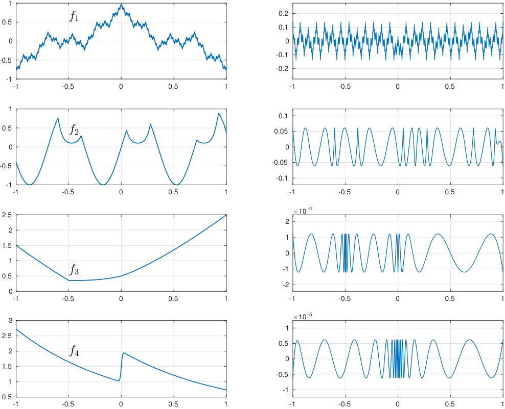
We have implemented22 2 The prototype code used is available at https://github.com/sfilip/barycentricDC. the barycentric DC algorithm in MATLAB using CVX [29] to specify the LP problems corresponding to (42)–(44), which are then solved using MOSEK’s [41] state-of-the-art LP optimizers. The four examples in Table 2 and Figure 10, for instance, demonstrate the effectiveness of the algorithm. For comparison, the sensitivity to the initial reference set prevented the convergence of our barycentric Remez implementation on all four of these examples. Function is particularly interesting since it is a version of Weierstrass’s classic example of a continuous but nowhere differentiable function.
Using a monomial or Chebyshev basis representation for the LP formulations quickly failed due to numerical errors, illustrating that the barycentric representation is crucial for the DC algorithm just as for the Remez algorithm.
We nevertheless echo the statement in the beginning of the section of the downsides of using the DC approach:
- •
Its overall cost. Producing the approximations in Figure 10 took several minutes in MATLAB on a desktop machine for each example.
- •
Numerical optimization tools for solving the corresponding LP problems break down at lower values of and than the ones we achieved with the barycentric Remez algorithm. We were usually able to go up to about type .
10 Minimax approximation in Chebfun
We have presented many algorithmic details that have enabled the design of a fast and robust Remez implementation. In closing we remind readers that all this is available in Chebfun and readily explored in a few lines of code. Download Chebfun version 5.7.0 or later from GitHub or www.chebfun.org, put it in your MATLAB path, and then try for example
      [p,q,r] = minimax(@(x) abs(x),60,60);
      fplot(@(x) abs(x)-r(x),[-1 1])
In a few seconds a beautiful curve with 123 exponentially clustered equioscillation points will appear. Figure 11 summarizes our algorithm in a flowchart.
References
- [1] Boost C++ Libraries. http://www.boost.org.
- [2] N. I. Akhiezer. Elements of the Theory of Elliptic Functions, volume 79 of Translations of Mathematical Monographs. American Mathematical Society, 1990.
- [3] I. Barrodale, M. J. D. Powell, and F. K. Roberts. The differential correction algorithm for rational -approximation. SIAM J. Numer. Anal., 9(3):493–504, 1972.
- [4] B. Beckermann. The condition number of real Vandermonde, Krylov and positive definite Hankel matrices. Numer. Math., 85(4):553–577, 2000.
- [5] B. Beckermann and A. Townsend. On the singular values of matrices with displacement structure. SIAM J. Matrix Anal. Appl., 38(4):1227–1248, 2017.
- [6] M. Berljafa and S. Güttel. The RKFIT algorithm for nonlinear rational approximation. SIAM J. Sci. Comp., 39(5):A2049–A2071, 2017.
- [7] J.-P. Berrut. Rational functions for guaranteed and experimentally well-conditioned global interpolation. Comput. Math. Appl., 15(1):1–16, 1988.
- [8] J.-P. Berrut, R. Baltensperger, and H. D. Mittelmann. Recent developments in barycentric rational interpolation. In Trends and Applications in Constructive Approximation, pages 27–51. Springer, 2005.
- [9] J.-P. Berrut and H. D. Mittelmann. Matrices for the direct determination of the barycentric weights of rational interpolation. J. Comput. Appl. Math., 78(2):355–370, 1997.
- [10] J.-P. Berrut and L. N. Trefethen. Barycentric Lagrange interpolation. SIAM Rev., 46(3):501–517, 2004.
- [11] D. Braess. Nonlinear Approximation Theory. Springer, 1986.
- [12] C. Brezinski and M. Redivo-Zaglia. Padé–type rational and barycentric interpolation. Numer. Math., 125(1):89–113, 2013.
- [13] F. Brophy and A. Salazar. Synthesis of spectrum shaping digital filters of recursive design. IEEE T. Circuits Syst., 22(3):197–204, 1975.
- [14] O. S. Celis. Practical Rational Interpolation of Exact and Inexact Data. PhD thesis, Universiteit Antwerpen, 2008.
- [15] E. Cheney. Introduction to Approximation Theory. AMS Chelsea Pub., 1982.
- [16] E. W. Cheney and H. L. Loeb. Two new algorithms for rational approximation. Numer. Math., 3(1):72–75, 1961.
- [17] A. K. Cline. Rate of convergence of Lawson’s algorithm. Math. Comp., 26(117):167–176, 1972.
- [18] W. J. Cody. The FUNPACK package of special function subroutines. ACM Trans. Math. Softw., 1(1):13–25, 1975.
- [19] W. J. Cody. Algorithm 715: SPECFUN—a Portable FORTRAN Package of Special Function Routines and Test Drivers. ACM Trans. Math. Softw., 19(1):22–30, 1993.
- [20] P. Cooper. Rational Approximation of Discrete Data with Asymptomatic Behaviour. PhD thesis, University of Huddersfield, 2007.
- [21] A. Curtis and M. R. Osborne. The construction of minimax rational approximations to functions. Comput. J., 9(3):286, 1966.
- [22] A. R. Curtis. Theory and calculation of best rational approximations. In Methods of Numerical Approximation, pages 139–148. Elsevier, 1966.
- [23] A. Deczky. Equiripple and minimax (Chebyshev) approximations for recursive digital filters. IEEE T. Acoust., Speech, Signal Process., 22(2):98–111, 1974.
- [24] T. A. Driscoll, N. Hale, and L. N. Trefethen. Chebfun Guide. Pafnuty Publications, Oxford, 2014.
- [25] S. N. Dua and H. L. Loeb. Further remarks on the differential correction algorithm. SIAM J. Numer. Anal., 10(1):123–126, 1973.
- [26] S. Ellacott and J. Williams. Linear Chebyshev approximation in the complex plane using Lawson’s algorithm. Math. Comp., 30(133):35–44, 1976.
- [27] M. S. Floater and K. Hormann. Barycentric rational interpolation with no poles and high rates of approximation. Numer. Math., 107(2):315–331, 2007.
- [28] I. J. Good. The colleague matrix, a Chebyshev analogue of the companion matrix. Q. J. Math., 12(1):61–68, 1961.
- [29] M. Grant and S. Boyd. CVX: Matlab software for disciplined convex programming, version 2.1. http://cvxr.com/cvx, Mar. 2014.
- [30] B. Gustavsen. Improving the pole relocating properties of vector fitting. IEEE Trans. Power Del., 21(3):1587–1592, 2006.
- [31] B. Gustavsen and A. Semlyen. Rational approximation of frequency domain responses by vector fitting. IEEE Trans. Power Del., 14(3):1052–1061, 1999.
- [32] R. Hettich and P. Zencke. An algorithm for general restricted rational Chebyshev approximation. SIAM J. Numer. Anal., 27(4):1024–1033, 1990.
- [33] N. J. Higham. Accuracy and Stability of Numerical Algorithms. SIAM, Philadelphia, PA, USA, second edition, 2002.
- [34] N. J. Higham. The numerical stability of barycentric Lagrange interpolation. IMA J. Numer. Anal., 24(4):547–556, 2004.
- [35]
A. C. Ioni
ă. Lagrange Rational Interpolation and its Applications to Approximation of Large-Scale Dynamical Systems. PhD thesis, Rice University, 2013.t , - [36] D. S. Karachalios. Hyperbolic function and the Loewner framework. private communication.
- [37] C. L. Lawson. Contributions to the Theory of Linear Least Maximum Approximations. PhD thesis, University of California, Los Angeles, 1961.
- [38] H. J. Maehly. Methods for fitting rational approximations, Parts II and III. J. ACM, 10(3):257–277, 1963.
- [39] A. J. Mayo and A. C. Antoulas. A framework for the solution of the generalized realization problem. Linear Algebra Appl., 425(2-3):634–662, 2007.
- [40] G. Meinardus. Approximation of Functions: Theory and Numerical Methods. Springer, 1967.
- [41] MOSEK ApS. The MOSEK optimization toolbox for MATLAB manual. Version 7.1 (Revision 28), 2015.
- [42] Y. Nakatsukasa and R. W. Freund. Computing fundamental matrix decompositions accurately via the matrix sign function in two iterations: The power of Zolotarev’s functions. SIAM Rev., 58(3):461–493, 2016.
- [43] Y. Nakatsukasa, O. Sète, and L. N. Trefethen. The AAA algorithm for rational approximation. Technical report, 2016. To appear in SIAM J. Sci. Comp.
- [44] Y. Nakatsukasa and L. N. Trefethen. Rational approximation of . Technical report, 2018. To appear in Proc. AMS.
- [45] D. J. Newman. Rational approximation to . Michigan Math. J., 11(1):11–14, 03 1964.
- [46] R. Pachón, R. B. Platte, and L. N. Trefethen. Piecewise-smooth chebfuns. IMA J. Numer. Anal., 30(4):898–916, 2010.
- [47] R. Pachón and L. N. Trefethen. Barycentric-Remez algorithms for best polynomial approximation in the Chebfun system. BIT Numer. Math., 49(4):721–741, 2009.
- [48] V. Y. Pan. How bad are Vandermonde matrices? SIAM J. Matrix Anal. Appl., 37(2):676–694, 2016.
- [49] A. Pelios. Rational function approximation as a well-conditioned matrix eigenvalue problem. SIAM J. Numer. Anal., 4(4):542–547, 1967.
- [50] M. J. D. Powell. Approximation Theory and Methods. Cambridge University Press, 1981.
- [51] A. Pushnitski and D. Yafaev. Best rational approximation of functions with logarithmic singularities. Constr. Approx., 46(2):243–269, 2017.
- [52] L. Reichel. Newton interpolation at Leja points. BIT Numer. Math., 30(2):332–346, 1990.
- [53] E. Remes. Sur le calcul effectif des polynômes d’approximation de Tchebichef. C. r. hebd. séances Acad. Sci., 199:337–340, 1934.
- [54] E. Remes. Sur un procédé convergent d’approximations successives pour déterminer les polynômes d’approximation. C. r. hebd. séances Acad. Sci., 198:2063–2065, 1934.
- [55] C. Schneider and W. Werner. Some new aspects of rational interpolation. Math. Comp., 47(175):285–299, 1986.
- [56] G. Stahl. Best uniform approximation of on . Russian Acad. Sci. Sb. Math., 76(2):461–487, 1993.
- [57] G. W. Stewart and J.-G. Sun. Matrix Perturbation Theory (Computer Science and Scientific Computing). Academic Press, 1990.
- [58] L. N. Trefethen. Approximation Theory and Approximation Practice. SIAM, 2013.
- [59] L. N. Trefethen and M. H. Gutknecht. The Carathéodory-Fejér method for real rational approximation. SIAM J. Numer. Anal., 20(2):420–436, 1983.
- [60] J. Van Deun. Computing near-best fixed pole rational interpolants. J. Comput. Appl. Math., 235(4):1077–1084, 2010.
- [61] J. Van Deun and L. N. Trefethen. A robust implementation of the Carathéodory–Fejér method for rational approximation. BIT Numer. Math., 51(4):1039–1050, 2011.
- [62] R. S. Varga, A. Ruttan, and A. D. Carpenter. Numerical results on best uniform rational approximation of on . Mathematics of the USSR-Sbornik, 74(2):271, 1993.
- [63] G. A. Watson. Approximation Theory and Numerical Methods. Wiley, 1980.
- [64] H. Werner. Die konstruktive Ermittlung der Tschebyscheff-Approximierenden im Bereich der rationalen Funktionen. Arch. Ration. Mech. An., 11(1):368–384, 1962.
- [65] H. Werner. Tschebyscheff-Approximation im Bereich der rationalen Funktionen bei Vorliegen einer guten Ausgangsnäherung. Arch. Ration. Mech. An., 10(1):205–219, 1962.