Isolated Loops in Quantum Feedback Networks

Let $\mathfrak{A}$ be a fixed algebra of operators, and let $M_{n,m}\left(\mathfrak{A}\right)$ denote the space of $n\times m$ arrays with entries in $\mathfrak{A}$. We say that $X=\left[X_{ij}\right]\in M_{n,m}\left(\mathfrak{A}\right)$ and $Y=\left[Y_{jk}\right]\in M_{m,r}\left(\mathfrak{A}\right)$ are composable, and define their product $XY\in M_{n,r}\left(\mathfrak{A}\right)$ via the row into column law of matrix multiplication - i.e., the $ik$ entry of $XY$ is $\sum_{j=1}^{r}X_{ij}Y_{jk}$.

In practice, $\mathfrak{A}$ will be a concrete algebra of operators on a fixed Hilbert space $\mathfrak{h}$ in which case elements of $M_{n,m}\left(\mathfrak{A}\right)$ may be thought of as operators from $\oplus^{m}\mathfrak{h}$ to $\oplus^{n}\mathfrak{h}$. Frequently, we will label rows and columns by index sets i and j and write $M_{\mathsf{ij}}\left(\mathfrak{A}\right)$ for the corresponding collection of arrays, and $\mathfrak{h}_{\mathsf{k}}=\oplus_{\mathsf{k}}\mathfrak{h}$. For instance, if we have a fixed index set $\mathsf{k}$ which is a disjoint union of $\mathsf{i}$ and $\mathsf{j}$, then we have the decomposition $\mathfrak{h}_{\mathsf{k}}\cong\mathfrak{h}_{\mathsf{i}}\oplus\mathfrak{h}_{\mathsf{j}}$, and for $X_{\mathsf{kk}}\in M_{\mathsf{kk}}\left(\mathfrak{A}\right)$ we have the corresponding block decomposition

with the sub-block $X_{\mathsf{ii}}$ belonging to $M_{\mathsf{ii}}\left(\mathfrak{A}\right)$, etc. Normally the index set $\mathsf{k}$ will be $\{1,2,\cdots,n\}$, however we have occasion to include an index 0. We will use notation such as $X_{0\mathsf{k}}\in M_{0\mathsf{k}}\left(\mathfrak{A}\right)$, for instance, to denote a row array $[X_{01},\cdots X_{0n}]$, etc.

Given a decomposition $X=\left[\begin{array}[]{cc}X_{\mathsf{aa}}&X_{\mathsf{ab}}\\ X_{\mathsf{ba}}&X_{\mathsf{bb}}\end{array}\right]$, we define the Schur complement of $X$ to be

where we shall always assume that $X_{\mathsf{bb}}$ is invertible as an operator on $\mathfrak{h}\otimes\mathbb{C}^{\mathsf{b}}$. Specifically, we say that this is the Schur complement of $X$ obtained by shortening the set of indices $\mathsf{b}$.

A key property that we shall use is that the order in which successive shortening of indices are applied is not important. In particular,

for any disjoint sets $\mathsf{b}_{1},\cdots,\mathsf{b}_{n}\subset\mathsf{j}$.

In the Markovian model of an open quantum system we consider a fixed Hilbert space $\mathfrak{h}_{0}$ for the system and a collection of independent quantum white noises $b_{k}\left(t\right)$ labeled by $k$ belonging to some discrete set $\mathsf{k}=\left\{1,\cdots,n\right\}$. That is, we have

The Schrödinger equation is

where the stochastic Hamiltonian takes the form

Here we assume that the $E_{\alpha\beta}$ are operators on $\mathfrak{h}_{0}$ with $E_{\alpha\beta}^{\ast}=E_{\beta\alpha}$. (In the course of this paper we will ignore technicalities related to unbounded operators.) We may write

where

with $E_{0\mathsf{k}}=\left[E_{01},\cdots,E_{0n}\right]$, $E_{\mathsf{k}0}=E_{0\mathsf{k}}^{{\dagger}}$ and $E_{\mathsf{kk}}$ the $n\times n$ matrix with entries $E_{jk}$ with $j,k\in\mathsf{k}$.

We may integrate the noises to get the following fundamental quantum stochastic processes:

The Schrödinger equation (2) is interpreted as the Stratonovich quantum stochastic differential equation

which may be readily converted into the quantum Itō form of Hudson and Parthasarathy. (In fact the latter is accomplished by Wick ordering the noise fields $b_{k}(t)$ and $b_{k}^{\ast}(t)$ in (2)[38].) The Stratonovich differentials may be algebraically defined as $X\left(t\right)\circ dY\left(t\right)=X\left(t\right)dY\left(t\right)+\frac{1}{2}dX\left(t\right).dY\left(t\right)$.

We obtain the general form of the constant operator coefficient quantum stochastic differential equation for an adapted unitary process $U(t)$:

where the $S_{jk},L_{j}$ and $H$ are operators on the initial Hilbert space, with $S_{\mathsf{kk}}=\left[S_{jk}\right]_{j,k\in\mathsf{k}}$ unitary, and $H$ self-adjoint. (We use the convention that $L_{\mathsf{k}}=\left[L_{k}\right]_{k\in\mathsf{k}}$ and that $L_{\mathsf{k}}^{\ast}L_{\mathsf{k}}=\sum_{k\in\mathsf{k}}L_{k}^{\ast}L_{k}$.) The triple $\left(S,L,H\right)$ are termed the Hudson-Parthasarathy parameters of the open system evolution. Explicitly, we have the relations

where Im$\,X$ means $\frac{1}{2i}\left(X-X^{\ast}\right)$.

We refer to this model as an SLH model, with $(S,L,H)$ being the Hudson-Parthasarathy parameters. We include closed systems, determined by a Hamiltonian operator $H$ within this category, and give the designation $(-,-,H)$.

We look at some special cases.

We consider an SLH system where we create a completely isolated loop by feeding all of the outputs back as inputs; see Figure 5. For convenience, we drop the label indices. The feedback reduction formula suggests that the resulting system is a closed Hamiltonian system, and using (60) and (62), the Hamiltonian will be

Here $Z=\frac{1}{2i}\frac{I+S}{I-S}$, as in (64). We see that $H_{\text{loop}}$ is indeed a self-adjoint operator provided $I-S$ is invertible (the well-posedness criterion for the feedback loop).

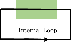
We re-derive (69) by considering the limit of a regular network with external inputs and outputs, leading to a completely isolated loop. This is represented in Figure 6 with an arbitrary component $\left(S_{0},L_{0},H_{0}\right)$ in loop.

The top component is a simple beam-splitter with a transmission coefficient $t$. Before making the feedback connections we have the open loop SLH model with

where

$\mathsf{e}$ labels the $n$ external channels, and $\mathsf{i}\equiv\mathsf{i}_{1}\cup\mathsf{i}_{2}$ where $\mathsf{i}_{1}$ are the remaining inputs into the beam-splitter and $\mathsf{i}_{2}$ the inputs into the component $\left(S_{0},L_{0},H_{0}\right)$. Also. the adjacency matrix (unitary gain) $\eta=\bigl[\begin{smallmatrix}0&I_{n}\\ I_{n}&0\end{smallmatrix}\bigr]$ is used in the feedback loop. Substituting into (47) leads to

The limit $t\rightarrow 0$ is well-defined and leads to

This we recognize as the SLH model where the input is trivially reflected - and so equals the output - while the Hamiltonian is modified exactly as in (69).

For two components $\left(S_{1},L_{1},H_{1}\right)$ and $\left(S_{2},L_{2},H_{2}\right)$ in series, we have the effective SLH component given by (II.3.1). Note that the first system drives the second and so the order is important.

Connecting them into an isolated loop, as in Figure 7, leads to the effective model $\left(\_,\_,H_{\text{loop}}\right)$ with

and the construction is well-posed so long as $I-S_{2}S_{1}$ is invertible.

One would naturally expect this Hamiltonian to be symmetric under interchange of the systems 1 and 2, and indeed it is not difficult to see that we may rearrange to get

We may also write this as

where the modified Hamiltonians of the components are

and we obtain an effective inter-component coupling

Suppose we wished to obtain a specific interaction $V_{12}$ between a pair of systems by setting up a loop. Let us suppose that we have

Substituting into (71), we find

where

In principle, we may set $\lambda$ to any desired value by adjusting $\phi_{1}$ and $\phi_{2}$. However, it is convenient to think of this as just a constant.

More generally we can have multiple loops with

and specified phases, so that

Theoretically we can approximate any interaction coupling.

In the special case of a cavity mode $a$ with frequency $\omega$ and damping rate $\gamma$ in series with a phase shifter $\left(S=e^{i\phi}\right)$, see Figure 8, we find that

where the shifted frequency is

The network is not well-posed when $\cos\phi=1$, so in particular we need a nontrivial phase shift $e^{i\phi}\neq 1$ in the loop. We see that the shifted frequency $\tilde{\omega}\left(\phi\right)$ can take any real value as $\phi$ varies between $0$ and $2\pi$. In effect, we have created a closed cavity with tunable resonant frequency.

Let us take two cavities with the SLH specifications $(S_{1}=e^{i\phi_{1}},L_{1}=\sqrt{\gamma_{1}}a_{1},H_{1}=\omega_{1}a_{1}^{\ast}a_{1})$, and $(S_{2}=e^{i\phi_{2}},L_{2}=\sqrt{\gamma_{2}}a_{2},H_{2}=\omega_{2}a_{2}^{\ast}a_{2})$.

The closed loop of Figure 9, will then have shifted frequencies for the two cavities, along with an additional interaction

where

and

Let us consider a two-level system with Hilbert space $\mathfrak{h}_{0}\cong\mathbb{C}^{2}$ coupled to a cavity mode with Hilbert space $\mathfrak{h}_{\text{mode}}$. The most general interaction possible can be written as

with respect to the factorization $\mathfrak{h}_{\text{mode}}\otimes\mathbb{C}^{2}$, and with $\sigma_{\pm},\sigma_{z}$ being the usual spin matrices. Here $V_{0},V_{\pm}$ and $V_{z}$ are operators on the Hilbert space $\mathfrak{h}_{\text{mode}}$ with $V_{0}^{\ast}=V_{0}$, $V_{\pm}^{\ast}=V_{\mp}$ and $V_{z}^{\ast}=V_{z}$. We shall take $V_{0}\equiv 0$ as this does not specify a coupling between the two-level system and the mode.

In order to realize the interaction, we could consider the two loops (i.e., the multiplicity $n=2$ in the loop in Figure 10) with

and scattering corresponding to phases $S_{1}=e^{i\phi_{1}}I_{2}$ and $S_{2}=e^{i\phi_{2}}I_{2}$ respectively. From (71), this leads to the interaction

with

and $f\left(\phi_{1},\phi_{2}\right)$ as in (75) above.

In particular, this leads to a way to engineer a Jaynes-Cummings interaction between the cavity mode and the two-level system with adjustable coupling constants.

References

- [1] S. Grivopoulos, I.R. Petersen, “Implementation of Bilinear Hamiltonian Interactions between Linear Quantum Stochastic Systems via Feedback.” Submitted to Automatica, arXiv:1609.05982 (2016)
- [2] J.E. Gough, M.R. James, Commun. Math. Phys. 287, 1109 (2009)
- [3] J.E. Gough, M.R. James, IEEE Trans. on Automatic Control 54(11), 2530-2544 (2009)
- [4] J. Combes, J. Kerckhoff, M. Sarovar, to appear in Advances in Physics, arXiv:1611.00375 (2016)
- [5] I. R. Petersen, Open Automation and Control Systems Journal 8, 67–93 (2016)
- [6] G. Zhang and M. James, Chinese Science Bulletin 57(18), 2200–2214, arxiv:1201.6020 (2012)
- [7] J.E. Gough, R. Gohm, M. Yanagisawa, ‘Phys. Rev. A 78, 062104 (2008)
- [8] J.E. Gough, M.R. James, H.I. Nurdin, Phys. Rev. A 81, 023804 (2010)
- [9] C. Gardiner and P. Zoller, Quantum Noise. Springer-Verlag, Berlin, second ed., 2000.
- [10] D. Walls and G. Milburn, Quantum Optics. Springer-Verlag, 2nd ed., 2008.
- [11] H. Wiseman and G. Milburn, Quantum Measurement and Control. Cambridge University Press, 2010.
- [12] A. Matyas, C. Jirauschek, F. Peretti, P. Lugli, and G. Csaba, IEEE Transactions on Microwave Theory and Techniques 59, 65–71 (2011)
- [13] J. Kerckhoff, R. W. Andrews, H. S. Ku, W. F. Kindel, K. Cicak, R. W. Simmonds, , and K. W. Lehnert, Physical Review X 3, 021013 (2013)
- [14] M. Tsang and C. M. Caves, Physical Review Letters 105, 123601 (2010)
- [15] F. Massel, T. T. Heikkilä, J. M. Pirkkalainen, S. U. Cho, H. Saloniemi, P. J. Hakonen, and M. A. Sillanpää, Nature 480, 351–354 (2011)
- [16] C. Dong, V. Fiore, M. C. Kuzyk, , and H. Wang, Science 338(6114), 1609–1613 (2012)
- [17] M. Yanagisawa, H. Kimura, IEEE Transactions on Automatic Control 48(12), 2107–2120, (2003)
- [18] M. Yanagisawa, H. Kimura, IEEE Transactions on Automatic Control 48(12), 2121–2132 (2003)
- [19] H. I. Nurdin, M. R. James, and I. R. Petersen, Automatica 45(8), 1837–1846 (2009)
- [20] M.R. James, H.I. Nurdin, & I.R. Petersen, IEEE Transactions on Automatic Control 53(8), 1787–1803 (2008)
- [21] A. I. Maalouf and I. R. Petersen, IEEE Transactions on Automatic Control 56(2), 309–319 (2011)
- [22] H. Mabuchi, Physical Review A 78, 032323 (2008)
- [23] R. Hamerly and H. Mabuchi, Physical Review Letters 109, 173602 (2012)
- [24] R. Hamerly and H. Mabuchi, Physical Review A 87, 013815 (2013)
- [25] O. Crisafulli, N. Tezak, D. B. S. Soh, M. A. Armen, and H. Mabuchi, Optics Express 21(15), 3761–3774 (2013)
- [26] H. I. Nurdin, M. R. James, and A. C. Doherty, SIAM Journal on Control and Optimization 48(4), 2686–2718 (2009)
- [27] H. I. Nurdin, IEEE Transactions on Automatic Control 55(10), 2439–2444 (2010)
- [28] H. I. Nurdin, ‘ IEEE Transactions on Automatic Control 55(4), 1008–1013 (2010)
- [29] H. I. Nurdin, S. Grivopoulos, and I. R. Petersen, Automatica 69, 324–333 (2016)
- [30] S. Grivopoulos and I. Petersen, “A realization method for transfer functions of linear quantum stochastic systems using static networks for input/output processing and feedback.” Submitted to SIAM Journal on Control and Optimization, arxiv:1511.04516 (2015)
- [31] Guofeng Zhang and Matthew R. James, IEEE Transactions on Automatic Control 56(7), 1535–1550 (2011)
- [32] Ian R. Petersen, “A direct coupling coherent quantum observer”, in Proceedings of the 2014 IEEE Multi-conference on Systems and Control, October 2014.
- [33] Ian R. Petersen and Elanor H. Huntington, “A reduced order direct coupling coherent quantum observer for a complex quantum plant”, in Proceedings of the 2016 European Control Conference.
- [34] Zibo Miao, Matthew R. James, and Valery A. Ugrinovskii, “Pole placement design for quantum systems via coherent observers”, In Proceedings of the 54th IEEE Conference on Decision and Control, December 2015.
- [35] Arash Kh. Sichani, Igor G. Vladimirov, and Ian R. Petersen, “Decentralized coherent quantum control design for translation invariant linear quantum stochastic networks with direct coupling”, in Proceedings of the 2015 Australian Control Conference, November 2015.
- [36] Ian R. Petersen and Elanor H. Huntington, “A possible implementation of a direct coupling coherent quantum observer”, in Proceedings of the 2015 Australian Control Conference, November 2015.
- [37] Ian R. Petersen and Elanor H. Huntington, “Implementation of a direct coupling coherent quantum observer including observer measurements”, in Proceedings of the 2016 American Control Conference, July 2016.
- [38] J. Gough, J. Math. Phys. 47, 113509 (2006)
- [39] J.E. Gough, J. Math. Phys. 57, 123505 (2016)
- [40] G. Tabak and H. Mabuchi, EPJ Quantum Technology 3:3, (2016)