A greedy approximation algorithm for the minimum $(2,2)$-connected dominating set problem

Suppose $G=(V,E)$ is a connected graph. A subset $C$ of $V$ is a said to be a connected dominating set (CDS) of $G$ if $G[C]$, the induced graph on $C$, is connected and every vertex $v$ in $V\setminus C$ is a neighbor of $C$ (connected by an edge to some vertex $u\in C$). Nodes in $C$ are called dominators, and nodes in $V\backslash C$ are called dominatees. To save energy and reduce interference, it is desirable that the CDS size is as small as possible. Computing a minimum CDS is a well known NP-hard problem [3]. By showing that finding a minimum set cover is a special case of finding a minimum CDS, Guha and Khullar [4] established that a minimum CDS can not be approximated within $\rho\ln n$ for any 0$<$$\rho<1$ unless $NP\subset DTIME(N^{O(\log\log n)}).$ In the same paper Guha and Khullar [4] proposed a two-phase greedy algorithm, with an approximation factor of $(3+\ln\Delta)$ for fining a minimum sized CDS. Subsequently, Ruan et. al. [5] used a potential function approach to come up with a single phase greedy algorithm improving the approximation ratio to $(2+\ln\Delta).$ There are, in the literature, several approximation algorithms for finding a minimum CDS for a general graph [2].

To make a virtual backbone more robust to deal with frequent node failures in WSNs, researchers have suggested using a $(k,m)$-CDS. As mentioned in the abstract, $C\subset V$ is a $(k,m)$-CDS if every node in $V\backslash C$ is adjacent to at least $m$ nodes in $C,$ and $G[C],$ the subgraph induced by $C,$ is $k$-connected. The $k$-connectedness means that $|C|>k$ and $G[C\backslash X]$ is connected for any $X\subset C$ with $|X|<k$. In other words, no two vertices of $G[C]$ are separated by removal of fewer than $k$ other vertices of $C$. With such a $C,$ messages can be shared by the whole network, where every node in $V\backslash C$ can tolerate up to $m-1$ faults (node failures) on its dominators, and the virtual backbone $G[C]$ can tolerate up to $k-1$ faults.

Zhou et al. [7], using a more complex potential function than the one in Ruan et al. [5], provide a single phase $(2+\ln(\Delta+m-2))$-approximation algorithm for the minimum $(1,m)$-CDS problem in a general graph.

Shi et al. [6], using a two-phase approach, provide a $(\alpha+2(1+\ln\alpha))$-approximation algorithm for the minimum $(2,m)$-CDS, where $m\geq 2$ and $\alpha$ is the approximation ratio for the computation of a $(1,m)$-CDS. Using the solution obtained for the minimum $(1,m)$-CDS problem, they augment the connectivity of $G[C]$ by merging blocks (a block is defined as a maximal connected subgraph without a cut-vertex) of $G[C]$ recursively. When $m=2,$ this approximation ratio becomes $(4+\ln\Delta+2\ln(2+\ln\Delta)).$

In this paper, we present a different two-phase approach to the $(2,2)$-CDS problem. The first phase ends up obtaining a $C$ such that it is a 2-fold dominating set, and all connected components of $G[C]$ are biconnected ($2$-connected). The second phase, at each iteration, needs two nodes from $V\backslash C$ to reduce the number of these biconnected components by at least one. This results in an algorithm with an asymptotic approximation factor of $(3+\ln(\Delta+2)).$ By a simple modification of the potential function, our approach provides a $(3+\ln(\Delta+m))$-approximation algorithm for computing a $(2,m)$-CDS.

For related and earlier work, the reader may refer to the papers by [6] and [7].

Let $G=(V,E)$ be a biconnected graph. For a $C\subset V,$ define $p(C)$ to be the number of (connected) components of $G[C],$ the subgraph induced by $C.$ Define $G\langle C\rangle$ to be the spanning subgraph of $G,$ with vertex set $V,$ and edge set $\{e\in E:e$ has at least one end in $C\}.$ Let $q(C)$ represents the number of components of $G\langle C\rangle.$ For each node $v\in V$, define $m_{C}(v)$ as:

Let $m(C)=\sum_{v\in V}m_{C}(v).$ Thus $m(C)$ represents the number of nodes in $V\backslash C$ which have at most one neighbor in $C.$ Note that for $m=2$, $q(C)$ and $m(C)$ are defined exactly as in [7]. Again, as in [7], we assign a color to each node in $V$ relative to a given $C$ as follows. All nodes in $C$ are colored black, nodes in $V\backslash C$ which have at least two neighbors in $C$ are colored gray, nodes in $V\backslash C$ that have exactly one neighbor in $C$ are colored red, and all other nodes are colored white.

Given $C$, we define $\hat{p}(C)$ to be

in an attempt to capture the bi-connectivity deficit of $G[C]$.

A node $x_{C}$ for which the maximum in (1) is attained is called a critical node of $C.$ case every node in $C$ can be viewed as a critical node.

Finally, we use the functions, $\hat{p}(C),q(C)$ and $m(C)$ to define a potential function, $f(C)$, on $C$ as:

and the difference function $\Delta_{y}f(C)$ by

where $y\in V.$ We can also, equivalently, write

1. 1.

   Suppose $y$ is gray. This means that $\hat{p}(C\cup\{y\})\leq\hat{p}(C)$. Clearly $m(C\cup\{y\})\leq m(C),$ and $q(C\cup\{y\})\leq q(C).$ Thus, $f(C\cup\{y\})\leq f(C),$ and hence $\Delta_{y}f(C)\geq 0.$

2. 2.

   Suppose $y$ is red. It is then connected to only one node in $C$. As $y$ is added to $C,$ its $m$-value goes down by one and its $q$-value cannot increase. Its $\hat{p}$ value may increase by $1$. Thus, $f(C\cup\{y\})\leq f(C)$.

3. 3.

   Suppose $y$ is white. As $y$ is added to $C$, its $m$-value goes down by one, $q$-value goes down by at least one, and $\hat{p}$-value goes up by one. Hence, $f(C\cup\{y\})\leq f(C)$.

The following characterization of the structure of a biconnected graph [1] is useful for us.

For example consider a biconnected graph that is a cycle $H$ of three nodes: $x_{1},x_{2},$ and $x_{3}.$ Then a path $P$ of three nodes $x_{1},x_{4},$ and $x_{3}$ is an $H$-path of $H.$ Adding this $H$-path to cycle $H$, keeps it biconnected. The following proposition formalizes this observation and is illustrated in Fig. 1

Suppose $C^{\ast}$ is a minimum $(2,2)$-CDS of $G.$ Since it is biconnected, using the above proposition we can list the nodes in an order such that each sublist starting from the beginning is essentially a “path”, where the first node of this “path” might correspond to a biconnected subgraph of $C^{\ast}.$ Let us illustrate this with the following example 2 of $G[C^{\ast}].$

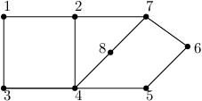
We can list 8 nodes of this graph as the following list with sublists: $((1,2,3,4),5,6,7),8).$ Node $2$ is adjacent to node $1,$ node $3$ is adjacent to only node $1.$ Node $4,$ however, is adjacent to both nodes $2$ and node $3.$ So $(1,2,3,4)$ corresponds to a biconnected graph (cycle), and is now designated as a “single meta-node” in our list. Next, the $H$-path $(4,5,6,7,2)$ is added to this subgraph, resulting in another biconnected subgraph. Finally, adding the $H$-path $(7,8,4)$ results in $G[C^{\ast}].$ The next lemma exploits this interpretation of a biconnected graph as a “path”.

The result is obvious if $y\in A.$ Suppose $y\in B\backslash A.$ Then the above result follows as $\Delta_{y}f(A)\geq 0$ for all $y\in V.$ Thus we assume from here on that $y\notin A\cup B.$ Define $\mu(f)=\Delta_{y}f(A\cup B)-\Delta_{y}f(A).$ It is useful to write $\mu(f)$ as:

We first look at $\mu(m).$ Define $S$ to be set of nodes which are neighbors of $y$ which are white with respect to $A$ and red with respect to $B$. Let $|S|=s.$ We first want to show that:

It is easy to formalize and establish this result by looking at the following two example figures: case (i): $\mu(m)=s-1,$ case (ii): $\mu(m)=s$.

In both 3(a) and 3(b) of Figure 3, $|S|=s=1.$ In Fig. 3(a), $m(A)=4,$ $m(A\cup\{y\})=3.$ Hence $\Delta_{y}m(A)=1.$ $m(A\cup B)=2,$ $m(A\cup B\cup\{y\})=1.$ Hence $\Delta_{y}m(A\cup B)=1.$ So $\mu(m)=\Delta_{y}m(A\cup B)-\Delta_{y}m(A)=0.$

In Fig. 3(b), $m(A)=4,$ $m(A\cup\{y\})=3.$ Hence $\Delta_{y}m(A)=1.$ $m(A\cup B)=3,m(A\cup B\cup\{y\})=1,$ $\Delta_{y}m(A\cup B)=2.$ Hence $\mu(m)=\Delta_{y}m(A\cup B)-\Delta_{y}m(A)=1.$

We now look at $\mu(q).$ We want to show that:

Let $N_{A}(y)$ be the set of components of $G\langle A\rangle$ that are adjacent with node $y$ in $G$ (the component of $G\langle A\rangle$ containing node $y$, if any, is not counted). Then $\Delta_{y}q(A)=|N_{A}(y)|.$ Hence $\mu(q)=|N_{A\cup B}(y)|-|N_{A}(y)|.$ Again, it is easy to formalize and establish the above result by looking at the above two example figures, in Figure 3, covering the cases: 3(a), $\mu(q)\leq-s,$ and 3(b): $\mu(q)\leq-(s-1)$.

In Figure 3(a), $\Delta_{y}q(A)=|N_{A}(y)|=3,$ $\Delta_{y}q(A\cup B)=N_{A\cup B}(y)=1.$ Hence $\mu(q)=1-3=-2.$

In Figure 3(b), $\Delta_{y}q(A)=N_{A}(y)=2,$ $\Delta_{y}q(A\cup B)=|N_{A\cup B}(y)|=1.$ Hence $\mu(q)=-1.$ Zhou et al. [7] have established the above two results in a more general setting.

Now we focus on $\mu(\hat{p})=\Delta_{y}\hat{p}(A\cup B)-\Delta_{y}\hat{p}(A)$.

Let $r$ be a critical node of $G[A]$. Let $A_{r}$ be the set of nodes in the component of $G[A]$ containing node $r.$ [Note that if $G[A]$ is connected then $A_{r}=A.$]

We define three constants $\alpha$, $\beta$, and $\gamma$ in $G[A]$ as follows. Let

$\alpha$ = $p(A_{r}\backslash\{r\}),$ the number of components in $G[A_{r}\backslash\{r\}].$

$\beta$ = The number of components $G[A\backslash A_{r}]$ which are adjacent to node $y$ in $G[A]$.

$\gamma$ = The number of components of $G[A_{r}\backslash\{r\}]$ which are are adjacent to node $y$ in $G[A].~(\gamma\leq\alpha)$.

Refer to Fig. 4 for an illustration.

Returning to $\mu(\hat{p})=\Delta_{y}\hat{p}(A\cup B)-\Delta_{y}\hat{p}(A)$, we use result-1 to make some assertions about $\mu(\hat{p})$. As we mentioned earlier, we can assume that $B$ is a set of nodes which form a “path”. Since $B$ is a “path”, adding $B$ to $A$ does not create a new critical node in $G[A\cup B]$.

Combining the three inequalities (4), (5), and (6), proves our Lemma 2.3.

Suppose $C=\emptyset$. We have $\hat{p}(\emptyset)=0,~q(\emptyset)=|V|,~m(\emptyset)=|V|.$ Since $G$ is biconnected, every node in $G$ has degree at least 2. Pick any node $y.$ So $C=\{y\},$ and $\hat{p}(\{y\})=0,$ $q(\{y\})=|V|-|N_{G}(y)|,$ $m(\{y\})=|V|.$ Hence $\Delta_{y}f(C)>0,$ a contradiction.

Suppose $m(C)>0.$ This means that there is at least one node $y$ which is red or white with respect to $C.$ Suppose that $y$ is a white node. This means that $y$ is an isolated node in $G\langle C\rangle,$ and hence accounts for one component in computing $q(C).$ Adding $y$ to $C$ implies $\Delta_{y}q(C)\geq 1,$ and $\Delta_{y}m(C)=1.$ Since $\Delta_{y}\hat{p}(C)\geq-1,$ we have $\Delta_{y}f(C)\geq 1,$ a contradiction. So assume that there are no white nodes. Suppose $y$ is red. This mean that $y$ is adjacent to only one node in $C.$ Since $G$ is biconnected, $y$ is adjacent to another node $y_{1}\notin C.$ So $y_{1}$ is either red or gray. Suppose $y_{1}$ is red. Adding $y$ to $C$ makes $y_{1}$ gray. Hence $\Delta_{y}m(C)=2.$ Since $\Delta_{y}q(C)\geq 0,$ and $\Delta_{y}\hat{p}(C)\geq-1,$ we have $\Delta_{y}f(C)\geq 1,$ a contradiction. So assume $y_{1}$ is gray. Then $\Delta_{y_{1}}\hat{p}(C)\geq 0,$ $\Delta_{y_{1}}m(C)=1,$ since $\ y$ is now gray in $G[C\cup\{y_{1}\}]$, $\Delta_{y_{1}}q(C)\geq 0,$ implying $\Delta_{y_{1}}f(C)>0,$ a contradiction. This proves the claim.

To prove this, suppose $C_{1}$ is a component of $C$ which is not biconnected. Hence $C_{1}$ has a critical vertex $x$ such that $\hat{p}(C_{1})=p(C_{1}\setminus\{x\})=t\geq 2$. Since $G$ is biconnected, there exists a gray node $y$ that is connected to two different components of $G[C_{1}\setminus\{x\}]$. Hence $\hat{p}(C_{1}\cup\{y\})\leq t-1$, implying $\Delta_{y}\hat{p}(C)\geq 1$, $\Delta_{y}q(C)\geq 0$, and hence $\Delta_{y}f(C)>0$, a contradiction.

When $\Delta_{y}f(C)=0$, $\forall$ $y\in V\setminus C$, we say that phase-I of the algorithm has ended. A formal description of the Phase I algorithm is given below. At the end of Phase I, $G[C]$ has $t$ biconnected components, $t\geq 1.$ If $t=1,$ there is nothing more to do. Again, since $G$ is biconnected, if $C_{1}$ and $C_{2}$ are any two components of $G[C]$, there must exist at least two nodes $y_{1}$ and $y_{2}$ in $V\setminus C$ such that both $y_{1}$ and $y_{2}$ are connected to both $C_{1}$ and $C_{2}$, making $G[C\cup\{y_{1},y_{2}\}]$ having one less component than $G[C]$.

So, if at the end of phase-I, we have $t$ components in $G[C]$, we need to add at most $2t$ nodes to $C$ to obtain a $(2,2)$-CDS.

Taking $i=1$, $C_{0}=\emptyset$. Then $\hat{p}(\emptyset)=0$, $q(\emptyset)=n$, $m(\emptyset)=n$. So $f(\emptyset)=2n$. $f(x_{1})=\hat{p}(\{x_{1}\})+q(\{x_{1}\})+m(\{x_{1}\})$, $\hat{p}(\{x_{1}\})=0$, $q(\{x_{1}\})=n-|N_{G}(x_{1})|-1$, $m(\{x_{1}\})=n-1$. This implies that $f(x_{1})=2n-2-|N_{G}(x_{1})|=2n-2-\Delta$. Hence

Now

So the approximation ratio asymptotically becomes $3+\ln(\Delta+2)$.

In this paper, we proposed a $(3+\ln(\Delta+2))$-approximation algorithm for the $(2,2)$-connected dominating set for a general graph. This algorithm can easily be generalized for the $(2,m)$-CDS problem, for $m\geq 2$, resulting in a $(3+\ln(\Delta+m))$-approximation algorithm.

References

- [1] Reinhard Diestel. Graph theory; 2nd ed. Graduate texts in mathematicals. Springer, Heidelberg, 2000. Record from the Electronic Library of Mathematics/European Mathematical Society.
- [2] Ding-Zhu Du, Ker-I Ko, and Xiaodong Hu. Design and Analysis of Approximation Algorithms. Springer Publishing Company, Incorporated, 2011.
- [3] Michael R. Garey and David S. Johnson. Computers and Intractability: A Guide to the Theory of NP-Completeness. W. H. Freeman & Co., New York, NY, USA, 1979.
- [4] Sudipto Guha and Samir Khuller. Approximation algorithms for connected dominating sets. Algorithmica, 20(4):374–387, 1998.
- [5] Lu Ruan, Hongwei Du, Xiaohua Jia, Weili Wu, Yingshu Li, and Ker-I Ko. A greedy approximation for minimum connected dominating sets. Theor. Comput. Sci., 329(1-3):325–330, 2004.
- [6] Yishuo Shi, Yaping Zhang, Zhao Zhang, and Weili Wu. A greedy algorithm for the minimum 2-connected m-fold dominating set problem. J. Comb. Optim., 31(1):136–151, 2016.
- [7] Jiao Zhou, Zhao Zhang, Weili Wu, and Kai Xing. A greedy algorithm for the fault-tolerant connected dominating set in a general graph. J. Comb. Optim., 28(1):310–319, 2014.