Residual Expansion Algorithm: Fast and Effective Optimization for
Nonconvex Least Squares Problems

We focus on nonconvex LS problems, of which many exist. In this paper, we study the following four important problems in computer vision and machine learning.

Most nonconvex optimization techniques are based on stochastic optimization, including GA [19], PSO [12], and SA [13]. These methods generally do not work well or require significant computation time for high-dimensional optimization problems. Several studies [4, 14, 18, 27, 24] have employed these nonconvex optimization techniques to our target problems described in Section 2.1; however, these methods are not often used in practice.

Our approach is related to graduated nonconvexity (GNC) [5], which first solves a simplified optimization problem and then gradually transforms the problem into the original nonconvex problem. The basic concept of graduated optimization methods is extinguishing local minima by using a convexified objective function, and then gradually changing the objective function to the original function. We refer readers to  [20] for a recent survey of graduated optimization. In contrast to GNC, our approach is explicitly to escape from poor local minima by using a largely expanded objective function and then gradually transforming it into the original function, as described in Section 4.

We consider one of the simplest cases: unconstrained and differentiable LS problems. Given a local optimum $\boldsymbol{\mathbf{\uptheta}}^{*}$, we can obtain first- and second-order derivatives of the $\alpha$-expanded objective function $E_{\alpha}\left(\boldsymbol{\mathbf{\uptheta}}\right)$ at $\boldsymbol{\mathbf{\uptheta^{*}}}$ as

where $J$ is a Jacobian matrix and $\boldsymbol{\mathbf{S}}\left(\boldsymbol{\mathbf{\uptheta}}^{*}\right)$ is

Eq. (11) means that $\boldsymbol{\mathbf{\uptheta}}^{*}$ is always a stationary point of $E_{\alpha}\left(\boldsymbol{\mathbf{\uptheta}}\right)$. Therefore, $\boldsymbol{\mathbf{\uptheta}}^{*}$ is a local minimum of $E_{\alpha}\left(\boldsymbol{\mathbf{\uptheta}}\right)$ if and only if $\nabla^{2}E_{\alpha}\left(\boldsymbol{\mathbf{\uptheta}}\right)$ is a positive semi-definite (PSD) matrix. If $\boldsymbol{\mathbf{S}}$ is not a PSD matrix, there is a $\alpha\geq 0$ which satisfies the fact that $\nabla^{2}E_{\alpha}\left(\boldsymbol{\mathbf{\uptheta}}\right)$ is not a PSD matrix.

Fig. 2 shows examples of $\alpha$-expanded objective functions. Residual expansion elevates the objective function around $\uptheta^{*}$, and if $\alpha$ is sufficiently large then it ceases to be a local minimum.

One-dimensional quartic minimization: Here we consider a quartic minimization problem—in particular, one that can be formulated as an LS problem:

We consider the case where Eq. (14) has two local minima $\theta_{1}$ and $\theta_{2}$. The following theorem then holds:

It is not obvious when our hypothesis, i.e., that a solution with a larger RE constant is closer to the global optimum, is valid. Unfortunately, we can easily find a counterexample in k-means clustering, as shown in Fig. 3. However, our algorithm, which aims to find a solution with a large RE constant, works well from an empirical perspective in many nonconvex LS problems.

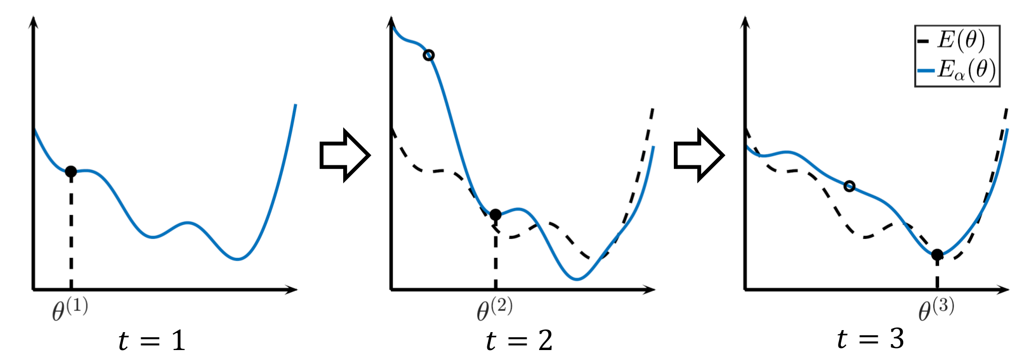
The RE algorithm has two parameters, $\alpha$ and $p$, for each iteration. We decrease $\alpha^{(t)}$ to 0 for convergence. when $\alpha=0$, there is no residual expansion and RE algorithm is guaranteed to converge if the original LS problem has a convergence-guaranteed algorithm. However, inadequate parameters of $\alpha$ and $p$ cause unstable optimization. We consider the norm of $\boldsymbol{\mathbf{r}}^{(t+1)}$. We can obtain

We use $\boldsymbol{\mathbf{f}}\left(\boldsymbol{\mathbf{\uptheta}}^{(t+1)}\right)\sim\hat{\boldsymbol{\mathbf{y}}}^{(t)}$ for the last approximation of Eq. (18). Eq. (18) suggests $\left(1-p-\alpha p\right)^{2}\leq 1$ to make the RE algorithm stable. A good way to determine these values of $\alpha$ and $p$ is described in Section 5.

Our algorithm consists of two steps of parameter updating and residual expansion. Parameter updating is based simply on a typical LS problem approach. Therefore, if there is a source code which minimizes Eq. (8), for example, by alternative optimization or gradient methods, then we can implement our algorithm by adding a residual expansion step to the existing code, which can be done in a few lines of code.

Moreover, the computational complexity of residual expansion is generally less than that of parameter updating. Therefore, we can achieve faster optimization than most nonconvex optimization techniques based on multi-point search or random search, such as SA and GA.

As described in Section 2.2, GNC is a similar approach to ours; however GNC often does not apply for LS problems. Our algorithm can be applied for any nonconvex LS problem provided that there is a method for finding a local optimum, such as Lloyd’s algorithm for k-means clustering and ICP algorithms for point-set registration.

We can simplify Eq. (21), Eq. (22) and Eq. (23) as

Details of the derivation are described in the supplementary material. This is a special case of the RE algorithm of Eq. (16) and Eq. (17) with

There are two main advantages to using ADMM. First, we can choose only $\mu$ instead of parameters $\alpha$ and $p$ in the general RE algorithm. Eq. (26) and Eq. (27) always satisfy $(1-p-\alpha p)^{2}<1$, which is a condition necessary for avoiding divergence to infinity, as described in Section 4.1, and this update achieves good performance in experiments. Second, ADMM can treat regularized LS optimization problems, such as blind image deblurring (Eq. (7)). We will describe this in the next section.

We consider a regularized LS problem as follows:

When we apply the RE algorithm in a straightforward manner, we can obtain the following objective function in each iteration:

In the case of ADMM, from Eq. (24), the objective function is as follows:

We can find that the difference between Eq. (29) and Eq. (30) is simply the coefficient of the squared term. We find that minimizing Eq. (30) achieves better performance than minimizing Eq. (29). We summarize the RE algorithm based on ADMM in Alg. 2.

We compared our method with k-means++ [2], which is a good initialization method, and Hartigan’s algorithm [10]. For Hartigan’s algorithm, we first used Lloyd’s algorithm [17] with k-means++ initialization for fast computation. We reported the total time of Lloyd’s algorithm and Hartigan’s algorithm. For the other method, we used Lloyd’s algorithm for optimization. We used random initialization for the RE algorithm. For error measurement, we used the objective function value of Eq. (1) and reported relative error from the value of k-means++ (therefore, the relative error of k-means++ is always 1).

We compared the RE algorithm with the ICP algorithm and Go-ICP [29]. Go-ICP is known as a method that can achieve global optimization. We used the bunny model from the Stanford3D dataset⁵⁵ 5 http://graphics.stanford.edu/data/3Dscanrep/, as in Fig. 6. For the target model, we used a partial point set as in Fig. 6(b). In the experiments, point sets were normalized within a cube of $[-1,1]^{3}$.

We made a rotation matrix $\boldsymbol{\mathbf{R}}_{gt}$ from a random rotation axis and the rotation angle $\phi$. The target point set was constructed by this rotation matrix, and we added Gaussian noise with a standard deviation of $\sigma=0.03$. We performed 50 tests with different random rotation axes at each rotation angle $\phi=\pi/3,5\pi/12,\pi/2$. For measurement of the error, we used the objective value Eq. (2) and regarded the results as successful if the objective error was less than 1 (this value is approximately twice of the average objective value using Go-ICP, as in Fig. 7).

We first show the comparison results between the RE algorithm and the ICP algorithm as in Table 4. The RE algorithm with $T=30$ achieved a better success rate with almost the same number of iterations as the ICP algorithm. Using a large $T$ can improve the results to a small extent.

We also compare our method to Go-ICP [29]. Go-ICP has two steps: the ICP algorithm and the branch-and-bound algorithm. We compared the original Go-ICP and RE + Go-ICP, which has the two steps of ICP with the RE and branch-and-bound algorithms. Fig. 7 plots all 50 results in $\phi=5\pi/12$. Note that this comparison was implemented entirely in C++. Go-ICP always found the global optimum solution; however, it required significant computation. RE + Go-ICP reduced computational cost while achieving global optimization.

We show that the RE algorithm is successful in OPQ optimization problems. We compare our method with the alternating optimization method [9, 22]. For a dataset, we used SIFT 1M [11], which contains 100,000 128-dimensional SIFT descriptors for training. We set the subspace number $M=8$ and cluster number $k=256$, which are often used in the field of approximate nearest neighbor search. For error measurement, we used the objective function value of Eq. (2.1.3). For our method, we set $\mu^{(0)}=0.5$.

We plot the objective function value versus iteration number in Fig. 8. We performed five repetitions using different initializations and report the average objective values obtained. Our method improved the objective function value; moreover, it achieved rapid convergence in the cases of $T=30$ and $T=100$. The RE algorithm elevates the objective function around the current solution; in other words, it transforms the gradient for the current solution into a steeper gradient, potentially causing rapid convergence.

We evaluated our method with single blind image deblurring. There are many formulations for blind image deblurring. In this paper, we followed Pan et al.’s formulation [23], which can be minimized by alternating optimization. We compared three methods as follows: a coarse-to-fine strategy [23] and RE algorithms based on Alg. 1 and Alg. 2. We used the uniform blurred text images from the dataset provided by Lai et al. [16], which contains five latent images and four blurring kernels for a total of 20 blurred images. For all methods, we used the same objective function parameters, such as the regularization coefficients. For our method, we set $\mu^{(0)}=0.2$ and $T=100$.

We show the results in Table 5. Our method significantly outperforms Pan’s method [23] and is successful for a significantly blurred image, as in Fig. 9. We found that Alg. 2 is superior to Alg. 1 in the cases of {image #3, kernel #4} and {image #5, kernel #4}. Note that these results are obtained by minimizing the same objective function, however using different optimization methods. Therefore our method likely improves upon other methods which use different objective functions [15, 28].

References

- [1] R. Achanta, A. Shaji, K. Smith, A. Lucchi, P. Fua, and S. Süsstrunk. SLIC superpixels compared to state-of-the-art superpixel methods. TPAMI, 34(11):2274–2282, 2012.
- [2] D. Arthur and S. Vassilvitskii. k-means++: The advantages of careful seeding. In SODA, pages 1027–1035, 2007.
- [3] P. J. Besl and H. D. McKay. A method for registration of 3-D shapes. TPAMI, 14(2):239–256, 1992.
- [4] G. Blais and M. D. Levine. Registering multiview range data to create 3D computer objects. TPAMI, 17(8):820–824, 1995.
- [5] A. Blake and A. Zisserman. Visual reconstruction. MIT Press, 1987.
- [6] S. Boyd, N. Parikh, E. Chu, B. Peleato, and J. Eckstein. Distributed optimization and statistical learning via the alternating direction method of multipliers. Foundations and Trends in Machine Learning, 3(1):1–122, 2011.
- [7] S. Cho and S. Lee. Fast motion deblurring. ACM ToG, 28(5):145:1–145:8, 2009.
- [8] G. Csurka, C. Dance, L. Fan, J. Willamowski, and C. Bray. Visual categorization with bags of keypoints. In In Workshop on Statistical Learning in Computer Vision, ECCV, pages 1–22, 2004.
- [9] T. Ge, K. He, Q. Ke, and J. Sun. Optimized product quantization for approximate nearest neighbor search. In CVPR, pages 2946–2953, 2013.
- [10] J. A. Hartigan. Clustering algorithms. John Wiley & Sons, Inc., 1975.
- [11] H. Jegou, M. Douze, and C. Schmid. Product quantization for nearest neighbor search. TPAMI, 33(1):117–128, 2011.
- [12] J. Kennedy and R. Eberhart. Particle swarm optimization. In ICNN, volume 4, pages 1942–1948, 1995.
- [13] S. Kirkpatrick, M. P. Vecchi, et al. Optimization by simmulated annealing. science, 220(4598):671–680, 1983.
- [14] K. Krishna and M. N. Murty. Genetic K-means algorithm. IEEE Transactions on Systems, Man, and Cybernetics, Part B (Cybernetics), 29(3):433–439, 1999.
- [15] D. Krishnan, T. Tay, and R. Fergus. Blind deconvolution using a normalized sparsity measure. In CVPR, pages 233–240, 2011.
- [16] W.-S. Lai, J.-B. Huang, Z. Hu, N. Ahuja, and M.-H. Yang. A comparative study for single image blind deblurring. In CVPR, June 2016.
- [17] S. Lloyd. Least squares quantization in PCM. TIT, 28(2):129–137, 1982.
- [18] J. Luck, C. Little, and W. Hoff. Registration of range data using a hybrid simulated annealing and iterative closest point algorithm. In ICRA, volume 4, pages 3739–3744, 2000.
- [19] M. Mitchell. An introduction to genetic algorithms. MIT press, 1998.
- [20] H. Mobahi and J. W. Fisher III. On the link between gaussian homotopy continuation and convex envelopes. In International Workshop on Energy Minimization Methods in CVPR, pages 43–56, 2015.
- [21] S. A. Nene, S. K. Nayar, H. Murase, et al. Columbia object image library (COIL-20). Technical report.
- [22] M. Norouzi and D. J. Fleet. Cartesian k-means. In CVPR, pages 3017–3024, 2013.
- [23] J. Pan, Z. Hu, Z. Su, and M.-H. Yang. Deblurring text images via l0-regularized intensity and gradient prior. In CVPR, pages 2901–2908, 2014.
- [24] L. Silva, O. R. P. Bellon, and K. L. Boyer. Precision range image registration using a robust surface interpenetration measure and enhanced genetic algorithms. TPAMI, 27(5):762–776, 2005.
- [25] N. Slonim, E. Aharoni, and K. Crammer. Hartigan’s k-means versus Lloyd’s k-means: Is it time for a change? In IJCAI, pages 1677–1684, 2013.
- [26] M. Telgarsky and A. Vattani. Hartigan’s method: k-means clustering without Voronoi. In AISTATS, pages 820–827, 2010.
- [27] M. P. Wachowiak, R. Smolíková, Y. Zheng, J. M. Zurada, and A. S. Elmaghraby. An approach to multimodal biomedical image registration utilizing particle swarm optimization. TEVC, 8(3):289–301, 2004.
- [28] L. Xu, S. Zheng, and J. Jia. Unnatural L0 sparse representation for natural image deblurring. In CVPR, pages 1107–1114, 2013.
- [29] J. Yang, H. Li, and Y. Jia. Go-ICP: Solving 3D registration efficiently and globally optimally. In ICCV, pages 1457–1464, 2013.