跳到论文正文
W Papers独立论文阅读器 arXiv:1705.09442 论文正文 计算阅读时间 · 0%
引用这篇论文根据当前论文元数据生成,正式投稿前建议核对。


License: arXiv.org perpetual non-exclusive license
arXiv:1705.09442v2 [math.AP] 19 Oct 2017

Well-posedness of the Goursat problem and stability for point source inverse backscattering

Eemeli Blåsten ††thanks: HKUST Jockey Club Institute for Advanced Study, Hong Kong University of Science and Technology, Hong Kong SAR. Email: iaseemeli@ust.hk
Abstract

We show logarithmic stability for the point source inverse backscattering problem under the assumption of angularly controlled potentials. Radial symmetry implies Hölder stability. Importantly, we also show that the point source equation is well-posed and also that the associated characteristic initial value problem, or Goursat problem, is well-posed. These latter results are difficult to find in the literature in the form required by the stability proof.

MSC classes: 35R30, 78A46, 35A08, 35L15

Keywords: inverse backscattering, point source, Goursat problem, stability

1 Introduction

For a potential function qq supported inside the unit disc BB in ℝ3\mathbb{R}^{3} and a point aa consider the point source problem

(∂t2−Δ−q)Ua(x,t)\displaystyle(\partial_{t}^{2}-\Delta-q)U^{a}(x,t) =δ⁡(x−a,t),\displaystyle=\delta(x-a,t), x∈ℝ3,t∈ℝ,\displaystyle x\in\mathbb{R}^{3},t\in\mathbb{R}, (1)
Ua​(x,t)\displaystyle U^{a}(x,t) =0,\displaystyle=0, x∈ℝ3,t<0.\displaystyle x\in\mathbb{R}^{3},t<0. (2)

We define the point source backscattering data as the function (a,t)↦Ua​(a,t)(a,t)\mapsto U^{a}(a,t). This paper has two goals: to prove the well-posedness of (1)–(2), and then to solve the inverse problem of determining qq from the point source backscattering data Ua​(a,t)U^{a}(a,t) with a∈∂Ba\in\partial B and t>0t>0.

The ordinary inverse problem of backscattering for arbitrary potentials is a major open problem. In it the scattering amplitude A⁡(x^,θ,k)A(\hat{x},\theta,k) is measured for frequencies k∈ℝ+k\in\mathbb{R}_{+}, incident plane-wave directions |θ|=1\left\lvert\theta\right\rvert=1, and measurement direction x^=−θ\hat{x}=-\theta. The question is whether such data corresponds to a unique potential qq. This question has been solved in the time-domain for an admissible class of potentials in [RU1]. For a more in-depth review of earlier results please refer to [MU].

Traditional backscattering applications include radar, fault detection in fiber optics, Rutherford backscattering and X-ray backscattering (e.g. full-body scanners) among others. What’s common to all of these is that the measured object (or fault) is located far away from the wave source. From the point of view of the Rakesh-Uhlmann [RU1, RU2] techniques the classical backscattering problem in the time-domain behaves as the point source problem with source at infinity. This means that the problem (1)–(2) models a situation where the wave source is close to the object under investigation, for example in the order of a few wavelengths. Therefor our results imply that backscattering experiments would give useful information even when the object is close. For example one could imagine using the backscattering of sound, radio or elastic waves to find faults in an object of human scale.

Uniqueness for the inverse backscattering problem related to (1)–(2) was shown by Rakesh and Uhlmann for an admissible class of smooth potentials in [RU2]. We shall show stability for their method. In addition we will show that the direct problem is well-posed in the sense of Hadamard, including all the required norm estimates.

The question of well-posedness of the direct problem would seem well-known to the experts at first sight. However this result is very difficult to find in the literature for non-smooth potentials and with explicit norm estimates. We hope that future research on the topic finds the explicit proof convenient.

The main motivation for this paper is the proof of the following stability theorem. As in [RU1, RU2] it applies to a class of potentials whose differences are angularly controlled.

Theorem 1.1.

Let B=B⁡(0¯,1)⊂ℝ3B=B(\bar{0},1)\subset\mathbb{R}^{3} and fix positive a-priori parameters S,ℳ<∞S,\mathcal{M}<\infty and h<1h<1. Then there are ℭ,𝔇<∞\mathfrak{C},\mathfrak{D}<\infty with the following properties:

Let q1,q2∈Cc7​(B)q_{1},q_{2}\in{C^{7}_{c}(B)} with norm bounds ‖qj‖C7≤ℳ{\left\lVert q_{j}\right\rVert_{C^{7}}}\leq\mathcal{M}. Assume moreover that supp⁡q1\supp q_{1} and supp⁡q2\supp q_{2} are no closer than distance hh from ∂B\partial B. If q1−q2q_{1}-q_{2} is angularly controlled with constant SS, i.e.

∑i<j∫|x|=r|Ωi​j​(q1−q2)​(x)|2​𝑑σ​(x)≤S2​∫|x|=r|(q1−q2)​(x)|2​𝑑σ​(x)\sum_{i<j}\int_{\left\lvert x\right\rvert=r}\left\lvert\Omega_{ij}(q_{1}-q_{2})(x)\right\rvert^{2}d\sigma(x)\leq S^{2}\int_{\left\lvert x\right\rvert=r}\left\lvert(q_{1}-q_{2})(x)\right\rvert^{2}d\sigma(x) (3)

for any 0<r<10<r<1 where Ωi​j=xi∂j−xj∂i\Omega_{ij}=x_{i}\partial_{j}-x_{j}\partial_{i} are the angular derivatives, then we have the following conditional stability estimate

‖q1−q2‖L2({|x|=r})≤eℭ/r4‖U1a−U2a‖\left\lVert q_{1}-q_{2}\right\rVert_{L^{2}(\{\left\lvert x\right\rvert=r\})}\leq e^{\mathfrak{C}/r^{4}}\left\lVert U_{1}^{a}-U_{2}^{a}\right\rVert (4)

for any given positive rr. Here U1aU^{a}_{1} and U2aU^{a}_{2} are the unique solutions to the problem (1)–(2) given by Theorem 1.2 with a∈∂Ba\in\partial B, q=q1q=q_{1}, q=q2q=q_{2}, and

‖U1a−U2a‖2=sup0<τ<1∫|a|=1|∂τ(τ⁡(U1a−U2a)​(a,2​τ))|2​𝑑σ​(a)\left\lVert U_{1}^{a}-U_{2}^{a}\right\rVert^{2}=\sup_{0<\tau<1}\int_{\left\lvert a\right\rvert=1}\left\lvert\partial_{\tau}\big(\tau(U^{a}_{1}-U^{a}_{2})(a,2\tau)\big)\right\rvert^{2}d\sigma(a)

is the backscattering measurement norm that we impose.

A fortiori we get the logarithmic full-domain estimate

‖q1−q2‖L2​(B)≤𝔇(ln1‖U1a−U2a‖)−1/4\left\lVert q_{1}-q_{2}\right\rVert_{L^{2}(B)}\leq\mathfrak{D}\left(\ln\frac{1}{\left\lVert U_{1}^{a}-U_{2}^{a}\right\rVert}\right)^{-1/4} (5)

when ‖U1a−U2a‖<e−1\left\lVert U_{1}^{a}-U_{2}^{a}\right\rVert<e^{-1} and ‖q1−q2‖L2​(B)≤𝔇⁡‖U1a−U2a‖\left\lVert q_{1}-q_{2}\right\rVert_{L^{2}(B)}\leq\mathfrak{D}\left\lVert U_{1}^{a}-U_{2}^{a}\right\rVert otherwise.

If instead of angular control for q1−q2q_{1}-q_{2} we assume the stronger condition of radial symmetry, we have

‖q1−q2‖L2({|x|=r})≤ℭrα‖U1a−U2a‖\left\lVert q_{1}-q_{2}\right\rVert_{L^{2}(\{\left\lvert x\right\rvert=r\})}\leq\mathfrak{C}r^{\alpha}\left\lVert U_{1}^{a}-U_{2}^{a}\right\rVert

where α=α⁡(ℳ,h,B)\alpha=\alpha(\mathcal{M},h,B), and this implies the full domain Hölder estimate

‖q1−q2‖L2​(B)≤𝔇​‖U1a−U2a‖11+α.\left\lVert q_{1}-q_{2}\right\rVert_{L^{2}(B)}\leq\mathfrak{D}\left\lVert U_{1}^{a}-U_{2}^{a}\right\rVert^{\frac{1}{1+\alpha}}.

The proof of the above theorem is presented in Section 4 and is based on the innovative techniques from [RU2]. It starts with writing the data U1a​(a,2​τ)−U2a​(a,2​τ)U_{1}^{a}(a,2\tau)-U_{2}^{a}(a,2\tau) as an integral involving q1−q2q_{1}-q_{2} and solutions to (1)–(2). The linear part of this integral is the average of q1−q2q_{1}-q_{2} over spheres with centers on ∂B\partial B. Proposition 4.2 is key for inverting the linearised problem and its perturbations. The inversion formula to this, and to the corresponding linearized problem in plane-wave inverse backscattering — which is the Radon transform — is an ill-posed operator. Angular control and Grönwall’s inequality give uniqueness and logarithmic stability to the linearized problem, and also to the full nonlinear inverse problem.

From the point of view of applications the logarithmic stability seems unpleasant. If we knew in advance that q1=q2q_{1}=q_{2} in a fixed neighbourhood of the origin, then (4) would give us a Lipschitz stability estimate ‖q1−q2‖L2​(B)≤C⁡‖U1a−U2a‖\left\lVert q_{1}-q_{2}\right\rVert_{L^{2}(B)}\leq C\left\lVert U_{1}^{a}-U_{2}^{a}\right\rVert. However it is not clear under which conditions q1−q2q_{1}-q_{2} would stay angularly controlled if the origin was moved to another location, e.g. outside of their supports. The method of this paper and [RU1, RU2] is centered around angular control so further work should focus on understanding this condition. When the integrals that use this condition are ignored, as happens when q1−q2q_{1}-q_{2} is radially symmetric, we get Hölder stability.

It would be extremely surprising if Hölder stability was possible in general. The fixed frequency multi-static inverse problem is known to be exponentially ill-posed [Man]. Counting dimensions, this problem is overdetermined in ℝ3\mathbb{R}^{3} while the harder backscattering problem is determined. However no formal inference can be made since there is no known direct way of deducing the multi frequency (or time-domain) backscattering data from the fixed frequency multi-static data. Furter comments on this complex issue deserve a completely new study.

Showing the well-posedness of the direct problem (1)–(2) is a major effort. This has to be done for two reasons. Firstly because the proof of Theorem 1.1 requires norm-estimates related to the solution UaU^{a}. These estimates are lacking from the literature. Secondly, it makes sure that the backscattering data Ua​(a,t)U^{a}(a,t) is smooth enough for the above theorem to say anything meaningful.

Theorem 1.2.

Let n≥7n\geq 7 and B=B⁡(0¯,1)B=B(\bar{0},1) be the unit disc in ℝ3\mathbb{R}^{3}. Let q∈Ccn​(B)q\in{C^{n}_{c}(B)} and a∈∂Ba\in\partial B. Then the point source problem (1)–(2) has a unique solution UaU^{a} in the set of distributions of order nn. It is given by

Ua​(x,t)=δ⁡(t−|x−a|)4​π​|x−a|+H⁡(t−|x−a|)​ra​(x,t)U^{a}(x,t)=\frac{\delta(t-\left\lvert x-a\right\rvert)}{4\pi\left\lvert x-a\right\rvert}+H(t-\left\lvert x-a\right\rvert)r^{a}(x,t) (6)

where ra∈C1​(ℝ3×ℝ)r^{a}\in C^{1}(\mathbb{R}^{3}\times\mathbb{R}) and δ,H\delta,H are the Dirac-delta distribution and Heaviside function on ℝ\mathbb{R}. For any T>0T>0 and ℳ≥‖q‖C7\mathcal{M}\geq{\left\lVert q\right\rVert_{C^{7}}} it has the norm estimate

‖ra‖C1​(ℝ3×[0,T])≤CT,ℳ.\left\lVert r^{a}\right\rVert_{C^{1}(\mathbb{R}^{3}\times{[{0,T}]})}\leq C_{T,\mathcal{M}}. (7)

Moreover UaU^{a} is C1C^{1}-smooth outside the light cone t=|x−a|t=\left\lvert x-a\right\rvert. In particular the map (a,τ)↦Ua​(a,2​τ)(a,\tau)\mapsto U^{a}(a,2\tau) is well-defined ∂B×(0,1)→ℂ\partial B\times{({0,1})}\to\mathbb{C} and continuously differentiable in τ\tau. Furthermore

supa∈∂Bsup0<τ<1|∂τβ(U1a−U2a)​(a,2​τ)|≤Cℳ​‖q1−q2‖C7\sup_{a\in\partial B}\sup_{0<\tau<1}\left\lvert\partial_{\tau}^{\beta}(U_{1}^{a}-U_{2}^{a})(a,2\tau)\right\rvert\leq C_{\mathcal{M}}{\left\lVert q_{1}-q_{2}\right\rVert_{C^{7}}}

for solutions UjaU^{a}_{j} arising from two potentials qjq_{j}, j=1,2j=1,2 and for any β∈{0,1}\beta\in\{0,1\}.

The proof of the above will be done by a progressive wave expansion. This will lead us to a characteristic initial value problem called the Goursat problem. In [RU2] this problem was mentioned briefly with reference to [Rom]. Another well-known source on the point source problem is [Fri]. The former studies the point source problem in low regularity Sobolev spaces, which is not good enough since we need a uniform ∂t\partial_{t}-estimate. The latter suffers from too much generality and considers only C∞C^{\infty} smooth coefficients, without any norm estimates. Neither reference mentions the Goursat problem by name or defines it explicitly.

There are other sources, more focused on the Goursat problem. For example [Cag] is very detailed on the topic but seems to have slightly larger smoothness requirements than we do. See also [Bal1, Bal2] for a very detailed analysis but their model has a region removed from the middle of the characteristic cone. Therefor we shall also prove well-posedness of the Goursat problem.

Theorem 1.3.

For n∈ℕ,n≥5n\in\mathbb{N},n\geq 5 let q∈Cn​(ℝ3)q\in C^{n}(\mathbb{R}^{3}) and g∈Cn+2​(ℝ3)g\in C^{n+2}(\mathbb{R}^{3}) with the norm bounds ‖q‖Cn≤ℳ\left\lVert q\right\rVert_{C^{n}}\leq\mathcal{M} and ‖g‖Cn+2≤𝒩\left\lVert g\right\rVert_{C^{n+2}}\leq\mathcal{N}. Then there is a unique C1C^{1} solution uu to the problem

(∂t2−Δ−q)u\displaystyle(\partial_{t}^{2}-\Delta-q)u =0,\displaystyle=0, x∈ℝ3,t>|x|\displaystyle x\in\mathbb{R}^{3},t>\left\lvert x\right\rvert
u⁡(x,t)\displaystyle u(x,t) =g⁡(x),\displaystyle=g(x), x∈ℝ3,t=|x|.\displaystyle x\in\mathbb{R}^{3},t=\left\lvert x\right\rvert.

It is also in Cs​(ℝ3×ℝ)C^{s}(\mathbb{R}^{3}\times\mathbb{R}) where s=⌊n−23⌋s=\lfloor\frac{n-2}{3}\rfloor and satisfies

(∂t+∂r)u=∂rg,x∈ℝ3,t=|x|(\partial_{t}+\partial_{r})u=\partial_{r}g,\qquad x\in\mathbb{R}^{3},t=\left\lvert x\right\rvert

where ∂r=x|x|⋅∇x\partial_{r}=\frac{x}{\left\lvert x\right\rvert}\cdot\nabla_{x}.

For any T<∞T<\infty the solution has the norm estimate

‖u‖Cs​(ℝ3×[0,T])≤CT,n,ℳ​𝒩.\left\lVert u\right\rVert_{C^{s}(\mathbb{R}^{3}\times{[{0,T}]})}\leq C_{T,n,\mathcal{M}}\mathcal{N}.

Finally, if q1,q2∈Cn​(ℝ3)q_{1},q_{2}\in C^{n}(\mathbb{R}^{3}) and g1,g2∈Cn+2​(ℝ3)g_{1},g_{2}\in C^{n+2}(\mathbb{R}^{3}) then their corresponding solutions satisfy

‖u1−u2‖Cs​(ℝ3×[0,T])≤CT,n,ℳ,𝒩​(‖q1−q2‖Cn​(ℝ3)+‖g1−g2‖Cn+2​(ℝ3)).\left\lVert u_{1}-u_{2}\right\rVert_{C^{s}(\mathbb{R}^{3}\times{[{0,T}]})}\leq C_{T,n,\mathcal{M},\mathcal{N}}\big(\left\lVert q_{1}-q_{2}\right\rVert_{C^{n}(\mathbb{R}^{3})}+\left\lVert g_{1}-g_{2}\right\rVert_{C^{n+2}(\mathbb{R}^{3})}\big).

We will use the following notation for function spaces of continuous functions.

Definition 1.4.

Let s∈ℕs\in\mathbb{N} and X⊂ℝdX\subset\mathbb{R}^{d} for some d∈ℤ+d\in\mathbb{Z}_{+}. The set Cs​(X)C^{s}(X) contains all f:X→ℂf\colon X\to\mathbb{C} that are ss times continuously differentiable. A subscript of cc as in Ccs​(X)C^{s}_{c}(X) indicates compact support in XX.

Given s,τ∈ℕs,\tau\in\mathbb{N} we denote by Cs,τ​(ℝ3×ℝ)C^{s,\tau}(\mathbb{R}^{3}\times\mathbb{R}) the space of continuous functions f:ℝ3×ℝ→ℂf\colon\mathbb{R}^{3}\times\mathbb{R}\to\mathbb{C} for which ∂xα∂tβf\partial_{x}^{\alpha}\partial_{t}^{\beta}f is continuous when α1+α2+α3≤s\alpha_{1}+\alpha_{2}+\alpha_{3}\leq s and β≤τ\beta\leq\tau.

For estimates,

‖f‖Cs​(X)=∑|α|≤ssupp∈X|∂αf⁡(p)|\displaystyle\left\lVert f\right\rVert_{C^{s}(X)}=\sum_{\left\lvert\alpha\right\rvert\leq s}\sup_{p\in X}\left\lvert\partial^{\alpha}f(p)\right\rvert
‖f‖Cs,τ​(X)=∑|α|≤sβ≤τsup(x,t)∈X|∂xα∂tβf⁡(x,t)|\displaystyle\left\lVert f\right\rVert_{C^{s,\tau}(X)}=\sum_{\begin{subarray}{c}\left\lvert\alpha\right\rvert\leq s\\ \beta\leq\tau\end{subarray}}\sup_{(x,t)\in X}\left\lvert\partial_{x}^{\alpha}\partial_{t}^{\beta}f(x,t)\right\rvert

where α\alpha is a multi-index of appropriate dimension.

A-priori no uniform bounds are required above. The solution to the wave equation has finite speed of propagation so the qualitative statements of our results stay true even for continuous but unbounded functions.

2 Goursat problem

The goal of this section is simple: prove the well-posedness of the Goursat problem, including norm estimates of the solution with dependence on the potential qq and Dirichlet data gg on the characteristic cone. Before that we will show informally how the point source problem is reduced to the Goursat problem, or characteristic initial-boundary value problem. Lemma 3.1 validates these informal calculations.

If δ,H∈𝒟′​(ℝ)\delta,H\in\mathscr{D}^{\prime}(\mathbb{R}) are the delta-distribution and Heaviside function, then applying the operator ∂t2−Δ+q\partial_{t}^{2}-\Delta+q to the ansatz

Ua​(x,t)=δ⁡(t−|x−a|)4​π​|x−a|+H⁡(t−|x−a|)​ra​(x,t)U^{a}(x,t)=\frac{\delta(t-\left\lvert x-a\right\rvert)}{4\pi\left\lvert x-a\right\rvert}+H(t-\left\lvert x-a\right\rvert)r^{a}(x,t) (8)

gives

(∂t2−Δ−q)Ua=(∂t2−Δ)δ⁡(t−|x−a|)4​π​|x−a|−q⁡(x)​δ​(t−|x−a|)4​π​|x−a|\displaystyle(\partial_{t}^{2}-\Delta-q)U^{a}=(\partial_{t}^{2}-\Delta)\frac{\delta(t-\left\lvert x-a\right\rvert)}{4\pi\left\lvert x-a\right\rvert}-\frac{q(x)\delta(t-\left\lvert x-a\right\rvert)}{4\pi\left\lvert x-a\right\rvert}
+δ′​(t−|x−a|)​(ra−ra)+2​δ⁡(t−|x−a|)|x−a|​(|x−a|​∂tra+ra+(x−a)⋅∇ra)\displaystyle+\delta^{\prime}(t-\left\lvert x-a\right\rvert)(r^{a}-r^{a})+2\frac{\delta(t-\left\lvert x-a\right\rvert)}{\left\lvert x-a\right\rvert}\left(\left\lvert x-a\right\rvert\partial_{t}r^{a}+r^{a}+(x-a)\cdot\nabla r^{a}\right)
+H(t−|x−a|)(∂t2−Δ−q)ra.\displaystyle+H(t-\left\lvert x-a\right\rvert)(\partial_{t}^{2}-\Delta-q)r^{a}.

Now UaU^{a} will be a solution to (1)–(2) if

(∂t2−Δ−q)ra\displaystyle(\partial_{t}^{2}-\Delta-q)r^{a} =0,\displaystyle=0, x∈ℝ3,t>|x−a|,\displaystyle x\in\mathbb{R}^{3},t>\left\lvert x-a\right\rvert,
(|x−a|∂t+1+(x−a)⋅∇)ra\displaystyle\left(\left\lvert x-a\right\rvert\partial_{t}+1+(x-a)\cdot\nabla\right)r^{a} =q8​π,\displaystyle=\frac{q}{8\pi}, x∈ℝ3,t=|x−a|.\displaystyle x\in\mathbb{R}^{3},t=\left\lvert x-a\right\rvert.

However if F⁡(x)=|x−a|​ra​(x,|x−a|)F(x)=\left\lvert x-a\right\rvert r^{a}(x,\left\lvert x-a\right\rvert) then the chain rule shows that

x−a|x−a|⋅∇F=(|x−a|∂t+1+(x−a)⋅∇)ra(x,|x−a|)=q⁡(x)8​π\frac{x-a}{\left\lvert x-a\right\rvert}\cdot\nabla F=\left(\left\lvert x-a\right\rvert\partial_{t}+1+(x-a)\cdot\nabla\right)r^{a}(x,\left\lvert x-a\right\rvert)=\frac{q(x)}{8\pi} (9)

and solving for FF gives

ra​(x,|x|)=18​π​∫01q⁡(a+s⁡(x−a))​𝑑s.r^{a}(x,\left\lvert x\right\rvert)=\frac{1}{8\pi}\int_{0}^{1}q(a+s(x-a))ds. (10)

Proving the converse requires more assumptions, so we will skip it now. Instead we shall show that the Goursat problem

(∂t2−Δ−q)ra\displaystyle(\partial_{t}^{2}-\Delta-q)r^{a} =0,\displaystyle=0, x∈ℝ3,t>|x−a|,\displaystyle x\in\mathbb{R}^{3},t>\left\lvert x-a\right\rvert, (11)
ra\displaystyle r^{a} =g,\displaystyle=g, x∈ℝ3,t=|x−a|\displaystyle x\in\mathbb{R}^{3},t=\left\lvert x-a\right\rvert (12)

has a unique solution in C1C^{1} for any qq and gg smooth enough, and that this solution also satisfies the boundary condition (9) when gg is chosen from (10). Natural smoothness conditions are q∈Cnq\in C^{n} and g∈Cn+2g\in C^{n+2}.

Definition 2.1.

For k∈ℤk\in\mathbb{Z} define the function ℝ3×ℝ→ℝ\mathbb{R}^{3}\times\mathbb{R}\to\mathbb{R}

γk​(x,t)={(t2−|x|2)kk!,k∈ℕ0,k<0.\gamma^{k}(x,t)=\begin{cases}\frac{(t^{2}-\left\lvert x\right\rvert^{2})^{k}}{k!},&k\in\mathbb{N}\\ 0,&k<0\end{cases}.
Lemma 2.2.

For n∈ℕn\in\mathbb{N} let q∈Cn​(ℝ3)q\in C^{n}(\mathbb{R}^{3}) and g∈Cn+2​(ℝ3)g\in C^{n+2}(\mathbb{R}^{3}). Let m≤⌊n2⌋+1m\leq\lfloor\frac{n}{2}\rfloor+1 be an integer. Then define v:ℝ3×ℝ→ℂv\colon\mathbb{R}^{3}\times\mathbb{R}\to\mathbb{C} by

v⁡(x,t)=∑k=0mak​(x)​γk​(x,t)v(x,t)=\sum_{k=0}^{m}a_{k}(x)\gamma^{k}(x,t)

where the functions aka_{k} are defined as

a0​(x)\displaystyle a_{0}(x) =g⁡(x),ℝ3,\displaystyle=g(x),\qquad\mathbb{R}^{3}, (13)
ak+1​(x)\displaystyle a_{k+1}(x) =14​∫01sk+1​((q+Δ)​ak)​(x​s)​𝑑s,ℝ3.\displaystyle=\frac{1}{4}\int_{0}^{1}s^{k+1}\big((q+\Delta)a_{k}\big)(xs)ds,\qquad\mathbb{R}^{3}. (14)

Then ak∈Cn+2−2​k​(ℝ3)a_{k}\in C^{n+2-2k}(\mathbb{R}^{3}). They have the norm estimate

‖ak‖Cn+2−2​k​(ℝ3)≤(1+‖q‖Cn​(ℝ3)4)k​‖g‖Cn+2​(ℝ3).\left\lVert a_{k}\right\rVert_{C^{n+2-2k}(\mathbb{R}^{3})}\leq\left(\frac{1+\left\lVert q\right\rVert_{C^{n}(\mathbb{R}^{3})}}{4}\right)^{k}\left\lVert g\right\rVert_{C^{n+2}(\mathbb{R}^{3})}.

If q1,q2∈Cn​(ℝ3)q_{1},q_{2}\in C^{n}(\mathbb{R}^{3}) and g1,g2∈Cn+2​(ℝ3)g_{1},g_{2}\in C^{n+2}(\mathbb{R}^{3}) then for the corresponding sequences ak​1a_{k1} and ak​2a_{k2} we have

‖ak​1−ak​2‖Cn+2−2​k≤(1+ℳ)k​‖g1−g2‖Cn+2+k​(1+ℳ)k−1​𝒩​‖q1−q2‖Cn\left\lVert a_{k1}-a_{k2}\right\rVert_{C^{n+2-2k}}\leq\big(1+\mathcal{M}\big)^{k}\left\lVert g_{1}-g_{2}\right\rVert_{C^{n+2}}+k\big(1+\mathcal{M}\big)^{k-1}\mathcal{N}\left\lVert q_{1}-q_{2}\right\rVert_{C^{n}}

whenever ℳ≥‖qj‖Cn\mathcal{M}\geq\left\lVert q_{j}\right\rVert_{C^{n}} and 𝒩≥‖gj‖Cn+2\mathcal{N}\geq\left\lVert g_{j}\right\rVert_{C^{n+2}}· Moreover

(∂t2−Δ−q)v\displaystyle(\partial_{t}^{2}-\Delta-q)v =−(q+Δ)​am​γm,\displaystyle=-(q+\Delta)a_{m}\gamma^{m}, x∈ℝ3,t∈ℝ,\displaystyle x\in\mathbb{R}^{3},t\in\mathbb{R},
v⁡(x,t)\displaystyle v(x,t) =g⁡(x),\displaystyle=g(x), x∈ℝ3,t=±|x|.\displaystyle x\in\mathbb{R}^{3},t=\pm\left\lvert x\right\rvert.
Proof.

Let us start by showing the norm estimates. Obviously a0∈Cn+2​(ℝ3)a_{0}\in C^{n+2}(\mathbb{R}^{3}) with estimate ‖a0‖Cn+2=‖g‖Cn+2\left\lVert a_{0}\right\rVert_{C^{n+2}}=\left\lVert g\right\rVert_{C^{n+2}} and a0​j→a0a_{0j}\to a_{0} in norm. Assume that ak∈Cn+2−2​ka_{k}\in C^{n+2-2k}. Then q​akqa_{k} has smoothness min⁡(n,n+2−2​k)\min(n,n+2-2k), and Δ​ak\Delta a_{k} has smoothness n−2​kn-2k. Hence ak+1a_{k+1} has smoothness n−2​kn-2k at worst, with norm estimate

‖ak+1‖Cn−2​k≤14​(1+‖q‖Cn)​‖ak‖Cn+2−2​k\left\lVert a_{k+1}\right\rVert_{C^{n-2k}}\leq\frac{1}{4}(1+\left\lVert q\right\rVert_{C^{n}})\left\lVert a_{k}\right\rVert_{C^{n+2-2k}}

whose coefficient could be improved by taking into account the value of the integral ∫01sk+1​𝑑s\int_{0}^{1}s^{k+1}ds. The norm estimate for a general kk is

‖ak‖Cn+2−2​k≤(1+‖q‖Cn4)k​‖g‖Cn+2\left\lVert a_{k}\right\rVert_{C^{n+2-2k}}\leq\left(\frac{1+\left\lVert q\right\rVert_{C^{n}}}{4}\right)^{k}\left\lVert g\right\rVert_{C^{n+2}}

by induction.

For the difference we note that

(a(k+1)​1−a(k+1)​2)​(x)=14​∫01sk+1​((q1+Δ)​ak​1−(q2+Δ)​ak​2)​(x​s)​𝑑s\big(a_{(k+1)1}-a_{(k+1)2}\big)(x)=\frac{1}{4}\int_{0}^{1}s^{k+1}\big((q_{1}+\Delta)a_{k1}-(q_{2}+\Delta)a_{k2}\big)(xs)ds

and thus

‖a(k+1)​1−a(k+1)​2‖Cn−2​k\displaystyle\left\lVert a_{(k+1)1}-a_{(k+1)2}\right\rVert_{C^{n-2k}}
≤(1+‖q1‖Cn)​‖ak​1−ak​2‖Cn+2−2​k+‖q1−q2‖Cn​‖ak​2‖Cn−2​k\displaystyle\qquad\leq(1+\left\lVert q_{1}\right\rVert_{C}^{n})\left\lVert a_{k1}-a_{k2}\right\rVert_{C^{n+2-2k}}+\left\lVert q_{1}-q_{2}\right\rVert_{C^{n}}\left\lVert a_{k2}\right\rVert_{C^{n-2k}}
≤(1+ℳ)​‖ak​1−ak​2‖Cn+2−2​k+(1+ℳ)k​𝒩​‖q1−q2‖Cn\displaystyle\qquad\leq\big(1+\mathcal{M}\big)\left\lVert a_{k1}-a_{k2}\right\rVert_{C^{n+2-2k}}+\big(1+\mathcal{M}\big)^{k}\mathcal{N}\left\lVert q_{1}-q_{2}\right\rVert_{C^{n}}

in terms of the a-priori bounds. The norm estimate for the difference is now a simple induction.

The claim (∂t2−Δ−q)v=−(q+Δ)amγm(\partial_{t}^{2}-\Delta-q)v=-(q+\Delta)a_{m}\gamma^{m} follows from noting that a0=ga_{0}=g, 4​x⋅∇ak+1+4​(2+k)​ak+1−(q+Δ)​ak=04x\cdot\nabla a_{k+1}+4(2+k)a_{k+1}-(q+\Delta)a_{k}=0, and ∂tγk=2​t​γk−1\partial_{t}\gamma^{k}=2t\gamma^{k-1}, ∇γk=−2​x​γk−1\nabla\gamma^{k}=-2x\gamma^{k-1}, and then finally applying ∂t2−Δ−q\partial_{t}^{2}-\Delta-q to the definition of vv. ∎

Lemma 2.3.

Let n,τ∈ℕn,\tau\in\mathbb{N}, q∈Cn​(ℝ3)q\in C^{n}(\mathbb{R}^{3}) and F∈Cn,τ​(ℝ3×ℝ)F\in C^{n,\tau}(\mathbb{R}^{3}\times\mathbb{R}). Assume that F⁡(x,t)=0F(x,t)=0 when t<|x|t<\left\lvert x\right\rvert, and consider the problem

(∂t2−Δ−q)w\displaystyle(\partial_{t}^{2}-\Delta-q)w =F,\displaystyle=F, x∈ℝ3,t∈ℝ,\displaystyle x\in\mathbb{R}^{3},t\in\mathbb{R}, (15)
w\displaystyle w =0,\displaystyle=0, x∈ℝ3,t<0.\displaystyle x\in\mathbb{R}^{3},t<0. (16)

It has a solution w∈Cn,τ​(ℝ3×ℝ)w\in C^{n,\tau}(\mathbb{R}^{3}\times\mathbb{R}) which moreover vanishes on t<|x|t<\left\lvert x\right\rvert. Given T<∞T<\infty and ℳ≥‖q‖Cn​(ℝ3)\mathcal{M}\geq\left\lVert q\right\rVert_{C^{n}(\mathbb{R}^{3})} it satisfies

‖w‖Cn,τ​(ℝ3×[0,T])≤CT,n,ℳ​‖F‖Cs,τ​(ℝ3×[0,T])\left\lVert w\right\rVert_{C^{n,\tau}(\mathbb{R}^{3}\times{[{0,T}]})}\leq C_{T,n,\mathcal{M}}\left\lVert F\right\rVert_{C^{s,\tau}(\mathbb{R}^{3}\times{[{0,T}]})}

where

CT,n,ℳ=Cn,τ​∑m=0∞Cnm​ℳm​T2​(m+1)4m+1​(m+1)!​(m+2)!<∞C_{T,n,\mathcal{M}}=C_{n,\tau}\sum_{m=0}^{\infty}\frac{C_{n}^{m}\mathcal{M}^{m}T^{2(m+1)}}{4^{m+1}(m+1)!(m+2)!}<\infty

and Cn,τC_{n,\tau} and CnC_{n} are finite and depend only on the parameters in their indices.

Finally, given such q1,q2q_{1},q_{2} and F1,F2F_{1},F_{2} let w1,w2w_{1},w_{2} be the corresponding solutions. With the a-priori bounds ‖qj‖Cn​(ℝ3)≤ℳ\left\lVert q_{j}\right\rVert_{C^{n}(\mathbb{R}^{3})}\leq\mathcal{M} and ‖Fj‖Cn,τ​(ℝ3×[0,T])≤𝒩\left\lVert F_{j}\right\rVert_{C^{n,\tau}(\mathbb{R}^{3}\times{[{0,T}]})}\leq\mathcal{N} we have

‖w1−w2‖Cn,τ​(ℝ3×[0,T])≤CT,n,ℳ,𝒩​(‖F1−F2‖Cn,τ​(ℝ3×[0,T])+‖q1−q2‖Cn​(ℝ3))\left\lVert w_{1}-w_{2}\right\rVert_{C^{n,\tau}(\mathbb{R}^{3}\times{[{0,T}]})}\leq C_{T,n,\mathcal{M},\mathcal{N}}\big(\left\lVert F_{1}-F_{2}\right\rVert_{C^{n,\tau}(\mathbb{R}^{3}\times{[{0,T}]})}+\left\lVert q_{1}-q_{2}\right\rVert_{C^{n}(\mathbb{R}^{3})}\big)

where CT,n,ℳ,𝒩C_{T,n,\mathcal{M},\mathcal{N}} is finite and depends only on the parameters in its indices.

Proof.

Consider the operator

K​f​(x,t)=∫ℝ3f⁡(x−y,t−|y|)4​π​|y|​𝑑yKf(x,t)=\int_{\mathbb{R}^{3}}\frac{f(x-y,t-\left\lvert y\right\rvert)}{4\pi\left\lvert y\right\rvert}dy

giving (∂t2−Δ)Kf=f(\partial_{t}^{2}-\Delta)Kf=f for compactly supported distributions f∈ℰ′​(ℝ3×ℝ)f\in\mathscr{E}^{\prime}(\mathbb{R}^{3}\times\mathbb{R}) and K​f​(x,t)=0Kf(x,t)=0 for t<inftsupp⁡ft<\inf_{t}\supp f. This is also true for ff supported on |x|≤t\left\lvert x\right\rvert\leq t (see Theorem 4.1.2 in [Fri]) and then the integration area becomes |x−y|+|y|≤t\left\lvert x-y\right\rvert+\left\lvert y\right\rvert\leq t. By Lemma 5.4

|∂xα∂tβK​f​(x,t)|≤{supℝ3×]−∞,t[|∂xα∂tβf|t2−|x|28,t>|x|0,t≤|x|\left\lvert\partial_{x}^{\alpha}\partial_{t}^{\beta}Kf(x,t)\right\rvert\leq\begin{cases}\sup_{\mathbb{R}^{3}\times{]{{-\infty},t}[}}\left\lvert\partial_{x}^{\alpha}\partial_{t}^{\beta}f\right\rvert\frac{t^{2}-\left\lvert x\right\rvert^{2}}{8},&t>\left\lvert x\right\rvert\\ 0,&t\leq\left\lvert x\right\rvert\end{cases}

when ∂xα∂tβf\partial_{x}^{\alpha}\partial_{t}^{\beta}f is a continuous function. In essence K​fKf has the same smoothness properties as ff.

The equation (∂t2−Δ−q)w=F(\partial_{t}^{2}-\Delta-q)w=F with w=0w=0 for negative time is equivalent to w=K​F+K⁡(q​w)w=KF+K(qw). Set w0​(x,t)=K​F​(x,t)w_{0}(x,t)=KF(x,t) and wm+1=K⁡(q​wm)w_{m+1}=K(qw_{m}), and we will build the final solutions as

w=∑m=0∞wm.w=\sum_{m=0}^{\infty}w_{m}.

We see immediately by the properties of KK that wm∈Cn,τ​(ℝ3×ℝ)w_{m}\in C^{n,\tau}(\mathbb{R}^{3}\times\mathbb{R}) for all mm and that they vanish on t<|x|t<\left\lvert x\right\rvert. Moreover

|∂xα∂tβw0​(x,t)|≤supℝ3×[0,t]|∂xα∂tβF|​t2−|x|28\left\lvert\partial_{x}^{\alpha}\partial_{t}^{\beta}w_{0}(x,t)\right\rvert\leq\sup_{\mathbb{R}^{3}\times{[{0,t}]}}\left\lvert\partial_{x}^{\alpha}\partial_{t}^{\beta}F\right\rvert\frac{t^{2}-\left\lvert x\right\rvert^{2}}{8}

when t>|x|t>\left\lvert x\right\rvert and α1+α2+α3≤n\alpha_{1}+\alpha_{2}+\alpha_{3}\leq n, β≤τ\beta\leq\tau.

Let us prove the claim by induction. Assume that for any α1+α2+α3≤n\alpha_{1}+\alpha_{2}+\alpha_{3}\leq n and β≤τ\beta\leq\tau we have

|∂xα∂tβwm​(x,t)|≤Cm​‖q‖Cn​(ℝ3)m​‖F‖Cn,τ​(ℝ3×[0,t])​(t2−|x|2)m+1\left\lvert\partial_{x}^{\alpha}\partial_{t}^{\beta}w_{m}(x,t)\right\rvert\leq C_{m}\left\lVert q\right\rVert_{C^{n}(\mathbb{R}^{3})}^{m}\left\lVert F\right\rVert_{C^{n,\tau}(\mathbb{R}^{3}\times{[{0,t}]})}(t^{2}-\left\lvert x\right\rvert^{2})^{m+1} (17)

for some CmC_{m} which might depend on the other parameters. Then recall wm=0w_{m}=0 for t<|x|t<\left\lvert x\right\rvert and the definition of wm+1w_{m+1}. We get

|∂xα∂tβwm+1​(x,t)|=|∫ℝ3∂xα(q⁡(x−y)​∂tβwm​(x−y,t−|y|))4​π​|y|​𝑑y|\displaystyle\left\lvert\partial_{x}^{\alpha}\partial_{t}^{\beta}w_{m+1}(x,t)\right\rvert=\left\lvert\int_{\mathbb{R}^{3}}\frac{\partial_{x}^{\alpha}\big(q(x-y)\partial_{t}^{\beta}w_{m}(x-y,t-\left\lvert y\right\rvert)\big)}{4\pi\left\lvert y\right\rvert}dy\right\rvert
≤Cm​∑γ≤α(αγ)​‖q‖Cn​(ℝ3)m+1​‖F‖Cn,τ​(ℝ3×[0,t])\displaystyle\qquad\leq C_{m}\sum_{\gamma\leq\alpha}{\alpha\choose\gamma}\left\lVert q\right\rVert_{C^{n}(\mathbb{R}^{3})}^{m+1}\left\lVert F\right\rVert_{C^{n,\tau}(\mathbb{R}^{3}\times{[{0,t}]})}
⋅∫|x−y|+|y|≤t((t−|y|)2−|x−y|2)m+14​π​|y|​𝑑y\displaystyle\qquad\quad\cdot\int_{\left\lvert x-y\right\rvert+\left\lvert y\right\rvert\leq t}\frac{\big((t-\left\lvert y\right\rvert)^{2}-\left\lvert x-y\right\rvert^{2}\big)^{m+1}}{4\pi\left\lvert y\right\rvert}dy
=Cm​Cs,n4​(m+2)​(m+3)​‖q‖Cn​(ℝ3)m+1​‖F‖Cn,τ​(ℝ3×[0,t])​(t2−|x|2)m+2\displaystyle\qquad=\frac{C_{m}C_{s,n}}{4(m+2)(m+3)}\left\lVert q\right\rVert_{C^{n}(\mathbb{R}^{3})}^{m+1}\left\lVert F\right\rVert_{C^{n,\tau}(\mathbb{R}^{3}\times{[{0,t}]})}(t^{2}-\left\lvert x\right\rvert^{2})^{m+2}

where the last equality comes from Lemma 5.4, and where

Cn=max⁡∑γ≤α|α|≤n⁡(αγ).C_{n}=\max_{\left\lvert\alpha\right\rvert\leq n}\sum_{\gamma\leq\alpha}{\alpha\choose\gamma}.

We also have wm+1​(x,t)=0w_{m+1}(x,t)=0 for t<|x|t<\left\lvert x\right\rvert. Hence we have the recursion formula Cm+1=Cm​Cn/(4​(m+2)​(m+3))C_{m+1}=C_{m}C_{n}/(4(m+2)(m+3)) and C0=1/8C_{0}=1/8. This implies that (17) holds with

Cm=Cnm4m+1​(m+1)!​(m+2)!C_{m}=\frac{C_{n}^{m}}{4^{m+1}(m+1)!(m+2)!}

for m=0,1,…m=0,1,\ldots.

The series

∑m=0∞|∂xα∂tβwm​(x,t)|≤∑m=0∞Cnm​‖q‖Cn​(ℝ3)m​(t2−|x|2)m+14m+1​(m+1)!​(m+2)!​‖F‖Cn,τ​(ℝ3×[0,t])\sum_{m=0}^{\infty}\left\lvert\partial_{x}^{\alpha}\partial_{t}^{\beta}w_{m}(x,t)\right\rvert\leq\sum_{m=0}^{\infty}\frac{C_{n}^{m}\left\lVert q\right\rVert_{C^{n}(\mathbb{R}^{3})}^{m}(t^{2}-\left\lvert x\right\rvert^{2})^{m+1}}{4^{m+1}(m+1)!(m+2)!}\left\lVert F\right\rVert_{C^{n,\tau}(\mathbb{R}^{3}\times{[{0,t}]})}

converges uniformly for any t,|x|t,\left\lvert x\right\rvert under a given bound, so the function ww is well defined. Note that the extension of t2−|x|2t^{2}-\left\lvert x\right\rvert^{2} by zero to t<|x|t<\left\lvert x\right\rvert is continuous. Hence ∂xα∂tβw\partial_{x}^{\alpha}\partial_{t}^{\beta}w is continuous in ℝ3×ℝ\mathbb{R}^{3}\times\mathbb{R} when α1+α2+α3≤n\alpha_{1}+\alpha_{2}+\alpha_{3}\leq n and β≤τ\beta\leq\tau. Thus w∈Cn,τ​(ℝ3×ℝ)w\in C^{n,\tau}(\mathbb{R}^{3}\times\mathbb{R}).

The final claim, continuous dependence on qq and FF, follows from the previous estimates. Namely, we note that w1w_{1} and w2w_{2} satisfy the assumptions of the source term FF, and the difference w1−w2w_{1}-w_{2} solves

(∂t2−Δ−q1)(w1−w2)=F1−F2+(q1−q2)w2(\partial_{t}^{2}-\Delta-q_{1})(w_{1}-w_{2})=F_{1}-F_{2}+(q_{1}-q_{2})w_{2}

with w1−w2=0w_{1}-w_{2}=0 for t<|x|t<\left\lvert x\right\rvert. The Cn,τ​(ℝ3×[0,T])C^{n,\tau}(\mathbb{R}^{3}\times{[{0,T}]})-norm of the right-hand side is bounded above by

CT,n,ℳ​(‖F1−F2‖Cn,τ+‖q1−q2‖Cn​CT,n,ℳ​‖F2‖Cn,τ)C_{T,n,\mathcal{M}}\big(\left\lVert F_{1}-F_{2}\right\rVert_{C^{n,\tau}}+\left\lVert q_{1}-q_{2}\right\rVert_{C^{n}}C_{T,n,\mathcal{M}}\left\lVert F_{2}\right\rVert_{C^{n,\tau}}\big)

and the claim follows from the a-priori bound on F2F_{2}. ∎

Lemma 2.4.

Let u:ℝ3×ℝ→ℂu\colon\mathbb{R}^{3}\times\mathbb{R}\to\mathbb{C} be a C1C^{1}-function satisfying

(∂t2−Δ−q)u\displaystyle(\partial_{t}^{2}-\Delta-q)u =0,\displaystyle=0, x∈ℝ3,t>|x|\displaystyle x\in\mathbb{R}^{3},t>\left\lvert x\right\rvert
u⁡(x,t)\displaystyle u(x,t) =g⁡(x),\displaystyle=g(x), x∈ℝ3,t=|x|\displaystyle x\in\mathbb{R}^{3},t=\left\lvert x\right\rvert

for some q∈C0​(ℝ3)q\in C^{0}(\mathbb{R}^{3}) and g∈C1​(ℝ3)g\in C^{1}(\mathbb{R}^{3}). If g=0g=0 then u=0u=0 in |x|≤t\left\lvert x\right\rvert\leq t.

Proof.

Define

E⁡(t)=∫|x|≤t(|∂tu|2+|∇u|2+|u|2)​𝑑x.E(t)=\int_{\left\lvert x\right\rvert\leq t}(\left\lvert\partial_{t}u\right\rvert^{2}+\left\lvert\nabla u\right\rvert^{2}+\left\lvert u\right\rvert^{2})dx.

We would like to differentiate EE with respect to time, however the lack of continuous second derivatives prevents us from doing that directly. Let φε\varphi_{\varepsilon} be a mollifier and uε=φε∗uu_{\varepsilon}=\varphi_{\varepsilon}\ast u. Let Eε​(t)=∫|x|≤t(|∂tuε|2+|∇uε|2+|uε|2)​𝑑xE_{\varepsilon}(t)=\int_{\left\lvert x\right\rvert\leq t}(\left\lvert\partial_{t}u_{\varepsilon}\right\rvert^{2}+\left\lvert\nabla u_{\varepsilon}\right\rvert^{2}+\left\lvert u_{\varepsilon}\right\rvert^{2})dx. Then

Eε′​(t)=∫|x|=t(|∂tuε|2+|∇uε|2+|uε|2)​𝑑σ​(x)+2​ℜ​∫|x|≤t∂tuε⋅∂t2uε¯​𝑑x\displaystyle E_{\varepsilon}^{\prime}(t)=\int_{\left\lvert x\right\rvert=t}\big(\left\lvert\partial_{t}u_{\varepsilon}\right\rvert^{2}+\left\lvert\nabla u_{\varepsilon}\right\rvert^{2}+\left\lvert u_{\varepsilon}\right\rvert^{2}\big)d\sigma(x)+2\Re\int_{\left\lvert x\right\rvert\leq t}\partial_{t}u_{\varepsilon}\cdot\overline{\partial_{t}^{2}u_{\varepsilon}}dx
+2ℜ∫|x|≤t∇∂tuε⋅∇uε¯dx+2ℜ∫|x|≤t∂tuεuε¯dx.\displaystyle\qquad\quad+2\Re\int_{\left\lvert x\right\rvert\leq t}\nabla\partial_{t}u_{\varepsilon}\cdot\overline{\nabla u_{\varepsilon}}dx+2\Re\int_{\left\lvert x\right\rvert\leq t}\partial_{t}u_{\varepsilon}\overline{u_{\varepsilon}}dx.

Integration by parts shows that the third term is equal to

2​ℜ​∫|x|=tx|x|​∂tuε⋅∇uε¯​𝑑σ​(x)−2​ℜ​∫|x|≤t∂tuε​Δ​uε¯​𝑑x.2\Re\int_{\left\lvert x\right\rvert=t}\frac{x}{\left\lvert x\right\rvert}\partial_{t}u_{\varepsilon}\cdot\overline{\nabla u_{\varepsilon}}d\sigma(x)-2\Re\int_{\left\lvert x\right\rvert\leq t}\partial_{t}u_{\varepsilon}\overline{\Delta u_{\varepsilon}}dx.

By combining both equations above and using ∂t2uε−Δ​uε=φε∗(q​u)\partial_{t}^{2}u_{\varepsilon}-\Delta u_{\varepsilon}=\varphi_{\varepsilon}\ast(qu) we get

Eε′​(t)=∫|x|=t(|x|x|​∂tuε+∇uε|2+|uε|2)​𝑑σ​(x)\displaystyle E_{\varepsilon}^{\prime}(t)=\int_{\left\lvert x\right\rvert=t}\left(\left\lvert\frac{x}{\left\lvert x\right\rvert}\partial_{t}u_{\varepsilon}+\nabla u_{\varepsilon}\right\rvert^{2}+\left\lvert u_{\varepsilon}\right\rvert^{2}\right)d\sigma(x)
+2ℜ∫|x|≤t∂tuε(uε+φε∗(q​u))¯dx.\displaystyle\qquad\quad+2\Re\int_{\left\lvert x\right\rvert\leq t}\partial_{t}u_{\varepsilon}\overline{(u_{\varepsilon}+\varphi_{\varepsilon}\ast(qu))}dx.

Integrate this with respect to time. Since uε→uu_{\varepsilon}\to u in C1C^{1} locally as ε→0\varepsilon\to 0, we get

E⁡(t)=∫0t∫|x|=s(|x|x|​∂su+∇u|2+|u|2)​𝑑σ​(x)​𝑑s\displaystyle E(t)=\int_{0}^{t}\int_{\left\lvert x\right\rvert=s}\left(\left\lvert\frac{x}{\left\lvert x\right\rvert}\partial_{s}u+\nabla u\right\rvert^{2}+\left\lvert u\right\rvert^{2}\right)d\sigma(x)ds
+∫0t2ℜ∫|x|≤s(1+q¯)∂suu¯dxds.\displaystyle\qquad\quad+\int_{0}^{t}2\Re\int_{\left\lvert x\right\rvert\leq s}(1+\overline{q})\partial_{s}u\overline{u}dxds.

Let us deal with the boundary integral next. Define ub​(x)=u⁡(x,|x|)u_{b}(x)=u(x,\left\lvert x\right\rvert). Then calculus shows that ∇ub​(x)=(∇u+x|x|​∂tu)​(x,|x|)\nabla u_{b}(x)=(\nabla u+\frac{x}{\left\lvert x\right\rvert}\partial_{t}u)(x,\left\lvert x\right\rvert) because ∇|x|=x/|x|\nabla\left\lvert x\right\rvert=x/\left\lvert x\right\rvert· On the other hand the boundary condition of uu shows that ub=gu_{b}=g. Thus the formula inside the parenthesis above is equal to |∇g|2+|g|2\left\lvert\nabla g\right\rvert^{2}+\left\lvert g\right\rvert^{2}.

Note that ∫0t∫|x|=sf⁡(x)​𝑑x​𝑑s=∫|x|≤tf⁡(x)​𝑑x\int_{0}^{t}\int_{\left\lvert x\right\rvert=s}f(x)dxds=\int_{\left\lvert x\right\rvert\leq t}f(x)dx for time-independent functions ff. Then, since 2​ℜ⁡(A​B¯)≤|A|2+|B|22\Re(A\overline{B})\leq\left\lvert A\right\rvert^{2}+\left\lvert B\right\rvert^{2}, we get

E⁡(t)≤∫|x|≤t(|∇g|2+|g|2)​𝑑x+(1+‖q‖∞)​∫0t∫|x|≤s(|∂su|2+|u|2)​𝑑x​𝑑s.E(t)\leq\int_{\left\lvert x\right\rvert\leq t}\big(\left\lvert\nabla g\right\rvert^{2}+\left\lvert g\right\rvert^{2}\big)dx+(1+\left\lVert q\right\rVert_{\infty})\int_{0}^{t}\int_{\left\lvert x\right\rvert\leq s}\big(\left\lvert\partial_{s}u\right\rvert^{2}+\left\lvert u\right\rvert^{2}\big)dxds.

The last integral has the upper bound ∫0tE⁡(s)​𝑑s\int_{0}^{t}E(s)ds. Grönwall’s inequality, for example Appendix B.2.k in [Evans], shows that E⁡(t)=0E(t)=0 when g=0g=0. ∎

We are now ready to prove the well-posedness of the Goursat problem in the sense of Hadamard. Strictly speaking the same proof shows existence in C0C^{0} when q∈C2q\in C^{2}, g∈C4g\in C^{4}, but then we cannot guarantee uniqueness or the boundary identity that’s stated with ∂t\partial_{t} and ∂r\partial_{r}.

Proof of Theorem 1.3.

This is a consequence of the uniqueness of Lemma 2.4, the progressive wave expansion of Lemma 2.2 and the initial value problem of Lemma 2.3. Let m=⌊(n+1)/3⌋m=\lfloor(n+1)/3\rfloor, which has m≥2m\geq 2 and n≥2​m+1n\geq 2m+1, and set

v(x,t)=g(x)+a1(x)(t2−|x|2)+⋅+am(x)γm(x,t)v(x,t)=g(x)+a_{1}(x)(t^{2}-\left\lvert x\right\rvert^{2})+\cdot+a_{m}(x)\gamma^{m}(x,t) (18)

for (x,t)∈ℝ3×ℝ(x,t)\in\mathbb{R}^{3}\times\mathbb{R}, as in Lemma 2.2. We have ‖ak‖Cn+2−2​k≤Cn​(1+ℳ)k​𝒩\left\lVert a_{k}\right\rVert_{C^{n+2-2k}}\leq C_{n}(1+\mathcal{M})^{k}\mathcal{N} in ℝ3\mathbb{R}^{3}. Then v⁡(x,|x|)=g⁡(x)v(x,\left\lvert x\right\rvert)=g(x) but (∂t2−Δ−q)v=−(q+Δ)amγm(\partial_{t}^{2}-\Delta-q)v=-(q+\Delta)a_{m}\gamma^{m}.

Next let

F⁡(x,t)={(q+Δ)​am​(x)​γm​(x,t),t>|x|0,t≤|x|F(x,t)=\begin{cases}(q+\Delta)a_{m}(x)\gamma^{m}(x,t),&t>\left\lvert x\right\rvert\\ 0,&t\leq\left\lvert x\right\rvert\end{cases} (19)

be our source term for an initial value problem. We have (q+Δ)​am∈Cn−2​m​(ℝ3)(q+\Delta)a_{m}\in C^{n-2m}(\mathbb{R}^{3}), but χ{t>|x|}γm\chi_{\{t>\left\lvert x\right\rvert\}}\gamma^{m} is in Cm−1​(ℝ3×ℝ)C^{m-1}(\mathbb{R}^{3}\times\mathbb{R}). Hence F∈Cn0,τ0​(ℝ3×ℝ)F\in C^{n_{0},\tau_{0}}(\mathbb{R}^{3}\times\mathbb{R}) using the notation of Lemma 2.3 whenever n0+τ0≤m−1n_{0}+\tau_{0}\leq m-1 and n0≤min⁡(n−2​m,m−1)=m−1n_{0}\leq\min(n-2m,m-1)=m-1. In other words when n0+τ0≤sn_{0}+\tau_{0}\leq s. Given T>0T>0 the source has the estimate

‖F‖Cn0,τ0​(ℝ3×[0,T])≤CT,n,ℳ​𝒩.\left\lVert F\right\rVert_{C^{n_{0},\tau_{0}}(\mathbb{R}^{3}\times{[{0,T}]})}\leq C_{T,n,\mathcal{M}}\mathcal{N}.

We can also write out the estimate for vv now that the smoothness indices are fixed. Note that γk\gamma^{k} is infinitely smooth in ℝ3×ℝ\mathbb{R}^{3}\times\mathbb{R}, and ama_{m} has the worst smoothness among all the coefficient functions in (18). Thus

‖v‖Cn0,τ0​(ℝ3×[0,T])≤CT,n,ℳ​𝒩\left\lVert v\right\rVert_{C^{n_{0},\tau_{0}}(\mathbb{R}^{3}\times{[{0,T}]})}\leq C_{T,n,\mathcal{M}}\mathcal{N} (20)

too since n0≤mn_{0}\leq m and aka_{k} is independent of tt.

Let ww solve (∂t2−Δ−q)w=F(\partial_{t}^{2}-\Delta-q)w=F in ℝ3×ℝ\mathbb{R}^{3}\times\mathbb{R} with w=0w=0 for t<0t<0. Lemma 2.3 shows that such a ww exists in Cn0,τ0​(ℝ3×ℝ)C^{n_{0},\tau_{0}}(\mathbb{R}^{3}\times\mathbb{R}) and it has support on t≥|x|t\geq\left\lvert x\right\rvert. Given T>0T>0 it has the norm estimate

‖w‖Cn0,τ0​(ℝ3×[0,T])≤CT,n,ℳ​𝒩\left\lVert w\right\rVert_{C^{n_{0},\tau_{0}}(\mathbb{R}^{3}\times{[{0,T}]})}\leq C_{T,n,\mathcal{M}}\mathcal{N} (21)

by the estimate on FF.

Since s≥1s\geq 1 then F∈C0,1∩C1,0F\in C^{0,1}\cap C^{1,0} with support in t≥|x|t\geq\left\lvert x\right\rvert. This implies that ∂tw\partial_{t}w and ∇xw\nabla_{x}w are continuous. Since w=0w=0 when t<|x|t<\left\lvert x\right\rvert we see that (∂t+x|x|⋅∇x)w=0(\partial_{t}+\frac{x}{\left\lvert x\right\rvert}\cdot\nabla_{x})w=0 for t≤|x|t\leq\left\lvert x\right\rvert. Next consider vv. We see that on t=|x|t=\left\lvert x\right\rvert

∂tγk​(x,t)={2​t,k=1,0,k≠1\partial_{t}\gamma^{k}(x,t)=\begin{cases}2t,&k=1,\\ 0,&k\neq 1\end{cases}

and

∇xγk​(x,t)={−2​x,k=1,0,k≠1,\nabla_{x}\gamma^{k}(x,t)=\begin{cases}-2x,&k=1,\\ 0,&k\neq 1\end{cases},

so ∂tv=2​t​a1\partial_{t}v=2ta_{1} and ∇xv=∇g−2​x​a1​(x)\nabla_{x}v=\nabla g-2xa_{1}(x) if t=|x|t=\left\lvert x\right\rvert. This implies that

(∂t+x|x|⋅∇x)v=x|x|⋅∇g(x)\left(\partial_{t}+\frac{x}{\left\lvert x\right\rvert}\cdot\nabla_{x}\right)v=\frac{x}{\left\lvert x\right\rvert}\cdot\nabla g(x)

on t=|x|t=\left\lvert x\right\rvert.

If we set u=v+wu=v+w, then we see that u⁡(x,|x|)=g⁡(x)u(x,\left\lvert x\right\rvert)=g(x) and (∂t+∂r)u=∂rg(\partial_{t}+\partial_{r})u=\partial_{r}g on t=r=|x|t=r=\left\lvert x\right\rvert because ww is continuous in ℝ3×ℝ\mathbb{R}^{3}\times\mathbb{R} and supported on t≥|x|t\geq\left\lvert x\right\rvert. Moreover u∈Csu\in C^{s} since

‖u‖Cs​(ℝ3×[0,T])≤C​supn0+τ0≤s‖u‖Cn0,τ0​(ℝ3×[0,T])\left\lVert u\right\rVert_{C^{s}(\mathbb{R}^{3}\times{[{0,T}]})}\leq C\sup_{n_{0}+\tau_{0}\leq s}\left\lVert u\right\rVert_{C^{n_{0},\tau_{0}}(\mathbb{R}^{3}\times{[{0,T}]})}

and this gives us the required norm estimate from (20) and (21). Finally (∂t2−Δ−q)u=(∂t2−Δ−q)v+F=0(\partial_{t}^{2}-\Delta-q)u=(\partial_{t}^{2}-\Delta-q)v+F=0 on t>|x|t>\left\lvert x\right\rvert.

The estimate for the difference of solutions u1−u2u_{1}-u_{2} to two Goursat problems follows from the corresponding estimate for v1−v2v_{1}-v_{2} of Lemma 2.2 and for w1−w2w_{1}-w_{2} of Lemma 2.3. After using the latter note that

‖F1−F2‖Cn0,τ0≤CT,n​(1+ℳ)​‖am​1−am​2‖Cn0+‖q1−q2‖​‖am​2‖Cn0\left\lVert F_{1}-F_{2}\right\rVert_{C^{n_{0},\tau_{0}}}\leq C_{T,n}\big(1+\mathcal{M}\big)\left\lVert a_{m1}-a_{m2}\right\rVert_{C^{n_{0}}}+\left\lVert q_{1}-q_{2}\right\rVert\left\lVert a_{m2}\right\rVert_{C^{n_{0}}}

holds and thus can be estimated above by the norms of q1−q2q_{1}-q_{2} and g1−g2g_{1}-g_{2}. ∎

3 Well-posedness of the point source backscattering measurements

Now that the Goursat problem has been taken care of we can focus on the point source problem. We will show that given a Cc7​(B){C^{7}_{c}(B)} potential qq there is a unique solution to (1)–(2), and we can define the associated backscattering measurements. Moreover these measurements depend continuously on the potential, with linear modulus of continuity.

Lemma 3.1.

Let q∈Cc0​(B)q\in C^{0}_{c}(B) and a∈∂Ba\in\partial B. Let ra∈C1​(ℝ3×ℝ)r^{a}\in C^{1}(\mathbb{R}^{3}\times\mathbb{R}) solve the problem

(∂t2−Δ−q)ra\displaystyle(\partial_{t}^{2}-\Delta-q)r^{a} =0,\displaystyle=0, x∈ℝ3,t>|x−a|,\displaystyle x\in\mathbb{R}^{3},t>\left\lvert x-a\right\rvert,
(|x−a|∂t+1+(x−a)⋅∇)ra\displaystyle\left(\left\lvert x-a\right\rvert\partial_{t}+1+(x-a)\cdot\nabla\right)r^{a} =q8​π,\displaystyle=\frac{q}{8\pi}, x∈ℝ3,t=|x−a|.\displaystyle x\in\mathbb{R}^{3},t=\left\lvert x-a\right\rvert.

Define

Ua​(x,t)=δ⁡(t−|x−a|)4​π​|x−a|+H⁡(t−|x−a|)​ra​(x,t)U^{a}(x,t)=\frac{\delta(t-\left\lvert x-a\right\rvert)}{4\pi\left\lvert x-a\right\rvert}+H(t-\left\lvert x-a\right\rvert)r^{a}(x,t)

where δ,H∈𝒟′​(ℝ)\delta,H\in\mathscr{D}^{\prime}(\mathbb{R}) are the delta-distribution and Heaviside function. Then UaU^{a} is a solution to the point source problem (1)–(2).

Proof.

Take the above form of UaU^{a} as an ansatz and note that the first term is the Green’s function for ∂t2−Δ\partial_{t}^{2}-\Delta

(∂t2−Δ)δ⁡(t−|x−a|)4​π​|x−a|=δ(x−a,t)(\partial_{t}^{2}-\Delta)\frac{\delta(t-\left\lvert x-a\right\rvert)}{4\pi\left\lvert x-a\right\rvert}=\delta(x-a,t) (22)

by for example Theorem 4.1.1 in [Fri].

Since the function rar^{a} in our ansatz is a-priori only C1C^{1}, we will use a smoothened delta-distribution and Heaviside function. For ε>0\varepsilon>0 let δε:ℝ→ℝ\delta_{\varepsilon}\colon\mathbb{R}\to\mathbb{R} be smooth, supported in ]0,2​ε[{]{0,2\varepsilon}[}, positive, and ∫δε=1\int\delta_{\varepsilon}=1. Let Hε​(t)=∫−∞tδε​(s)​𝑑sH_{\varepsilon}(t)=\int_{-\infty}^{t}\delta_{\varepsilon}(s)ds. Then δε\delta_{\varepsilon} converges to the delta-distribution as ε→0\varepsilon\to 0 and HεH_{\varepsilon} to the Heaviside function. Let our new ansatz be

Uε​(x,t)=δε​(t−|x−a|)4​π​|x−a|+Hε​(t−|x−a|)​ra​(x,t).U_{\varepsilon}(x,t)=\frac{\delta_{\varepsilon}(t-\left\lvert x-a\right\rvert)}{4\pi\left\lvert x-a\right\rvert}+H_{\varepsilon}(t-\left\lvert x-a\right\rvert)r^{a}(x,t).

Let’s calculate the derivatives of the second term in the ansatz next. Note that ∇⋅(x/|x|)=2/|x|\nabla\cdot(x/\left\lvert x\right\rvert)=2/\left\lvert x\right\rvert in 3D, and so setting R=Hε​(t−|x−a|)​ra​(t,x)R=H_{\varepsilon}(t-\left\lvert x-a\right\rvert)r^{a}(t,x) we have

∂tR\displaystyle\partial_{t}R =δε​(t−|x−a|)​ra+Hε​(t−|x−a|)​∂tra\displaystyle=\delta_{\varepsilon}(t-\left\lvert x-a\right\rvert)r^{a}+H_{\varepsilon}(t-\left\lvert x-a\right\rvert)\partial_{t}r^{a}
∂t2R\displaystyle\partial_{t}^{2}R =δε′​(t−|x−a|)​ra+2​δε​(t−|x−a|)​∂tra+Hε​(t−|x−a|)​∂t2ra,\displaystyle=\delta_{\varepsilon}^{\prime}(t-\left\lvert x-a\right\rvert)r^{a}+2\delta_{\varepsilon}(t-\left\lvert x-a\right\rvert)\partial_{t}r^{a}+H_{\varepsilon}(t-\left\lvert x-a\right\rvert)\partial_{t}^{2}r^{a},
∇R\displaystyle\nabla R =δε(t−|x−a|)(−x−a|x−a|)ra+Hε(t−|x−a|)∇ra\displaystyle=\delta_{\varepsilon}(t-\left\lvert x-a\right\rvert)\left(-\frac{x-a}{\left\lvert x-a\right\rvert}\right)r^{a}+H_{\varepsilon}(t-\left\lvert x-a\right\rvert)\nabla r^{a}
Δ​R\displaystyle\Delta R =δε′​(t−|x−a|)​ra−δε​(t−|x−a|)​2​ra|x−a|\displaystyle=\delta_{\varepsilon}^{\prime}(t-\left\lvert x-a\right\rvert)r^{a}-\delta_{\varepsilon}(t-\left\lvert x-a\right\rvert)\frac{2r^{a}}{\left\lvert x-a\right\rvert}
−δε(t−|x−a|)2x−a|x−a|⋅∇ra+Hε(t−|x−a|)δεra,\displaystyle\phantom{=}-\delta_{\varepsilon}(t-\left\lvert x-a\right\rvert)2\frac{x-a}{\left\lvert x-a\right\rvert}\cdot\nabla r^{a}+H_{\varepsilon}(t-\left\lvert x-a\right\rvert)\delta_{\varepsilon}r^{a},
q​R\displaystyle qR =Hε​(t−|x−a|)​q​ra.\displaystyle=H_{\varepsilon}(t-\left\lvert x-a\right\rvert)qr^{a}.

Take all terms into account next. Then

(∂t2−Δ−q)Uε=(∂t2−Δ)δε​(t−|x−a|)4​π​|x−a|−q⁡(x)​δε​(t−|x−a|)4​π​|x−a|\displaystyle(\partial_{t}^{2}-\Delta-q)U_{\varepsilon}=(\partial_{t}^{2}-\Delta)\frac{\delta_{\varepsilon}(t-\left\lvert x-a\right\rvert)}{4\pi\left\lvert x-a\right\rvert}-\frac{q(x)\delta_{\varepsilon}(t-\left\lvert x-a\right\rvert)}{4\pi\left\lvert x-a\right\rvert}
+δε′​(t−|x−a|)​(ra−ra)+2​δε​(t−|x−a|)|x−a|​(|x−a|​∂tra+ra+(x−a)⋅∇ra)\displaystyle+\delta_{\varepsilon}^{\prime}(t-\left\lvert x-a\right\rvert)(r^{a}-r^{a})+2\frac{\delta_{\varepsilon}(t-\left\lvert x-a\right\rvert)}{\left\lvert x-a\right\rvert}\left(\left\lvert x-a\right\rvert\partial_{t}r^{a}+r^{a}+(x-a)\cdot\nabla r^{a}\right)
+Hε(t−|x−a|)(∂t2−Δ−q)ra.\displaystyle+H_{\varepsilon}(t-\left\lvert x-a\right\rvert)(\partial_{t}^{2}-\Delta-q)r^{a}.

As ε→0\varepsilon\to 0 the first term above converges to δ⁡(x−a,t)\delta(x-a,t) in the space of distributions. The terms with coefficients δε′\delta_{\varepsilon}^{\prime} and HεH_{\varepsilon} vanish. The former trivially, and the latter because our choice of δε\delta_{\varepsilon} makes sure that supp⁡Hε⊂ℝ+\supp H_{\varepsilon}\subset\mathbb{R}_{+}. In other words

limε→0(∂t2−Δ−q)Uε−δ(x−a,t)\displaystyle\lim_{\varepsilon\to 0}(\partial_{t}^{2}-\Delta-q)U_{\varepsilon}-\delta(x-a,t)
=limε→02​δε​(t−|x−a|)|x−a|​(|x−a|​∂tra+ra+(x−a)⋅∇ra−q⁡(x)8​π)\displaystyle\qquad=\lim_{\varepsilon\to 0}2\frac{\delta_{\varepsilon}(t-\left\lvert x-a\right\rvert)}{\left\lvert x-a\right\rvert}\left(\left\lvert x-a\right\rvert\partial_{t}r^{a}+r^{a}+(x-a)\cdot\nabla r^{a}-\frac{q(x)}{8\pi}\right)

in 𝒟′​(ℝ3×ℝ)\mathscr{D}^{\prime}(\mathbb{R}^{3}\times\mathbb{R}).

Denote by f⁡(x,t)f(x,t) the continuous function in parenthesis above. Let φ∈Cc∞​(ℝ3×ℝ)\varphi\in C^{\infty}_{c}(\mathbb{R}^{3}\times\mathbb{R}) be a test function. Then in the support of φ\varphi for every μ>0\mu>0 there is δ>0\delta>0 such that |f⁡(x,t)|<μ\left\lvert f(x,t)\right\rvert<\mu if |t−|x−a||<δ\left\lvert t-\left\lvert x-a\right\rvert\right\rvert<\delta. Let 2​ε<δ2\varepsilon<\delta. Then

|∫ℝ3×ℝδε​(t−|x−a|)|x−a|​f​(x,t)​φ​(x,t)​𝑑x​𝑑t|≤μ​‖φ‖∞​∫supp⁡φδε​(t−|x−a|)|x−a|​𝑑x​𝑑t\left\lvert\int_{\mathbb{R}^{3}\times\mathbb{R}}\frac{\delta_{\varepsilon}(t-\left\lvert x-a\right\rvert)}{\left\lvert x-a\right\rvert}f(x,t)\varphi(x,t)dxdt\right\rvert\leq\mu\left\lVert\varphi\right\rVert_{\infty}\int_{\supp\varphi}\frac{\delta_{\varepsilon}(t-\left\lvert x-a\right\rvert)}{\left\lvert x-a\right\rvert}dxdt

and by integrating the tt-variable first we get the upper bound

…≤μ​‖φ‖∞​∫B⁡(a,Rφ)d​x|x−a|=Cφ​μ.\ldots\leq\mu\left\lVert\varphi\right\rVert_{\infty}\int_{B(a,R_{\varphi})}\frac{dx}{\left\lvert x-a\right\rvert}=C_{\varphi}\mu.

In other words the remaining term in the expansion for (∂t2−Δ−q)Uε(\partial_{t}^{2}-\Delta-q)U_{\varepsilon} tends to zero in the distribution sense. Hence

(∂t2−Δ−q)Uε→δ(x−a,t)(\partial_{t}^{2}-\Delta-q)U_{\varepsilon}\to\delta(x-a,t)

in 𝒟′​(ℝ3×ℝ)\mathscr{D}^{\prime}(\mathbb{R}^{3}\times\mathbb{R}). Also, since supp⁡δε⊂ℝ+\supp\delta_{\varepsilon}\subset\mathbb{R}_{+}, it also satisfies the initial condition Uε=0U_{\varepsilon}=0 for t<0t<0. Finally, it is easy to see that Uε→UaU_{\varepsilon}\to U^{a}. Hence the latter is a solution to (1)–(2). ∎

Lemma 3.2.

For n∈ℕn\in\mathbb{N} let q∈Cn​(ℝ3)q\in C^{n}(\mathbb{R}^{3}) and let UU be a distribution of order nn on ℝ3×ℝ\mathbb{R}^{3}\times\mathbb{R} such that U=0U=0 on t<0t<0. If (∂t2−Δ−q)U=0(\partial_{t}^{2}-\Delta-q)U=0 then U=0U=0.

Proof.

Let φ∈Cc∞​(ℝ3×ℝ)\varphi\in C^{\infty}_{c}(\mathbb{R}^{3}\times\mathbb{R}) be arbitrary. There is x0∈ℝ3x_{0}\in\mathbb{R}^{3} and t0∈ℝt_{0}\in\mathbb{R} such that φ⁡(x,t)=0\varphi(x,t)=0 in |x−x0|>t0−t\left\lvert x-x_{0}\right\rvert>t_{0}-t, i.e. outside a past light cone. Write y=x−x0y=x-x_{0} and s=t0−ts=t_{0}-t, and define

Q⁡(y)=q⁡(y+x0),F⁡(y,s)=φ⁡(y+x0,t0−s).Q(y)=q(y+x_{0}),\qquad F(y,s)=\varphi(y+x_{0},t_{0}-s).

Then Q∈Cn​(ℝ3)Q\in C^{n}(\mathbb{R}^{3}), F∈Cc∞​(ℝ3×ℝ)F\in C^{\infty}_{c}(\mathbb{R}^{3}\times\mathbb{R}) and F⁡(y,s)=0F(y,s)=0 when s<|y|s<\left\lvert y\right\rvert. Lemma 2.3 gives the existence of w∈Cn​(ℝ3×ℝ)w\in C^{n}(\mathbb{R}^{3}\times\mathbb{R}) which vanishes on s<|y|s<\left\lvert y\right\rvert and satisfies (∂s2−Δ−Q)w=F(\partial_{s}^{2}-\Delta-Q)w=F.

Let

ψ⁡(x,t)=w⁡(x−x0,t0−t).\psi(x,t)=w(x-x_{0},t_{0}-t).

Then ψ⁡(x,t)=0\psi(x,t)=0 if |x−x0|>t0−t\left\lvert x-x_{0}\right\rvert>t_{0}-t. Since U=0U=0 for t<0t<0, the intersection of the supports of ψ\psi and UU is a compact set. Since UU is of order nn and ψ\psi is in CnC^{n} their distribution pairing ⟨U,ψ⟩\langle U,\psi\rangle is well defined. Now

⟨(∂t2−Δ−q)U,ψ⟩=⟨U,(∂t2−Δ−q)ψ⟩\displaystyle\langle(\partial_{t}^{2}-\Delta-q)U,\psi\rangle=\langle U,(\partial_{t}^{2}-\Delta-q)\psi\rangle
=⟨U~,(∂s2−Δ−Q)w⟩=⟨U~,F⟩=⟨U,φ⟩\displaystyle\qquad=\langle\tilde{U},(\partial_{s}^{2}-\Delta-Q)w\rangle=\langle\tilde{U},F\rangle=\langle U,\varphi\rangle

where U~\tilde{U} is the distribution UU in the (y,s)(y,s)-coordinates. Since UU is in the kernel of the differential operator and φ\varphi is an arbitrary test function, we have U=0U=0. ∎

Proof of Theorem 1.2.

Uniqueness follows directly from Lemma 3.2. We shall build a solution rar^{a} to the Goursat-type problem of Lemma 3.1. We switch boundary conditions as was done at the beginning of Section 2. Define

g⁡(x)=18​π​∫01q⁡(a+s⁡(x−a))​𝑑sg(x)=\frac{1}{8\pi}\int_{0}^{1}q\big(a+s(x-a)\big)ds

and note that q∈Cn​(ℝ3)q\in C^{n}(\mathbb{R}^{3}), g∈Cn+2​(ℝ3)g\in C^{n+2}(\mathbb{R}^{3}) for n=5n=5. The well-posedness of the Goursat problem (Theorem 1.3) gives a unique C1C^{1} solution to

(∂t2−Δ−q)ra\displaystyle(\partial_{t}^{2}-\Delta-q)r^{a} =0,\displaystyle=0, x∈ℝ3,t>|x−a|,\displaystyle x\in\mathbb{R}^{3},t>\left\lvert x-a\right\rvert,
ra\displaystyle r^{a} =g,\displaystyle=g, x∈ℝ3,t=|x−a|.\displaystyle x\in\mathbb{R}^{3},t=\left\lvert x-a\right\rvert.

It has the required norm estimate for any T>0T>0 and in addition it satisfies

(∂t+∂r)ra=∂rg(\partial_{t}+\partial_{r})r^{a}=\partial_{r}g

on t=|x−a|t=\left\lvert x-a\right\rvert. Here r=|x−a|r=\left\lvert x-a\right\rvert and furthermore we denote θ=(x−a)/|x−a|\theta=(x-a)/\left\lvert x-a\right\rvert. If in the definition of gg we switch integration variables to s′=r​ss^{\prime}=rs then

∂rg=−1r​g+q8​π​r\partial_{r}g=-\frac{1}{r}g+\frac{q}{8\pi r}

which is well-defined because q=0q=0 in a neighbourhood of aa. Recalling that ∂r=θ⋅∇x\partial_{r}=\theta\cdot\nabla_{x} we see that in fact

(|x−a|∂t+1+(x−a)⋅∇x)ra=q8​π(\left\lvert x-a\right\rvert\partial_{t}+1+(x-a)\cdot\nabla_{x})r^{a}=\frac{q}{8\pi}

on the boundary t=|x−a|t=\left\lvert x-a\right\rvert. Hence Lemma 3.1 shows that UaU^{a} is a solution to the point source problem.

The unperturbed Green’s function is supported only on t=|x−a|t=\left\lvert x-a\right\rvert. On t<|x−a|t<\left\lvert x-a\right\rvert the solution vanishes. On t>|x−a|t>\left\lvert x-a\right\rvert it is equal to rar^{a} which is C1C^{1}. In this topology, it depends continuously on aa because the Goursat problem depends continuously on the potential and characteristic boundary data. Hence U⁡(a,2​τ)U(a,2\tau) is well-defined for τ>0\tau>0 and continuously differentiable in τ\tau.

Let two potentials q1q_{1} and q2q_{2} and their associated solutions r1ar_{1}^{a}, r2ar_{2}^{a} to the Goursat problem be given. For any a∈∂Ba\in\partial B and β∈{0,1}\beta\in\{0,1\} Theorem 1.3 shows the norm estimate

supx∈ℝ3sup0<τ<1|∂τβ(r1a−r2a)​(x,2​τ)|≤Cℳ​‖q1−q2‖C7\sup_{x\in\mathbb{R}^{3}}\sup_{0<\tau<1}\left\lvert\partial_{\tau}^{\beta}(r_{1}^{a}-r_{2}^{a})(x,2\tau)\right\rvert\leq C_{\mathcal{M}}{\left\lVert q_{1}-q_{2}\right\rVert_{C^{7}}}

because ‖g1−g2‖C7​(ℝ3)≤‖q1−q2‖C7​(ℝ3)\left\lVert g_{1}-g_{2}\right\rVert_{C^{7}(\mathbb{R}^{3})}\leq\left\lVert q_{1}-q_{2}\right\rVert_{C^{7}(\mathbb{R}^{3})} and the norms involved are invariant under translations. Letting x=ax=a and then taking the supremum over aa proves the claim because U1a−U2a=r1a−r2aU_{1}^{a}-U_{2}^{a}=r_{1}^{a}-r_{2}^{a} at (x,t)=(a,2​τ)(x,t)=(a,2\tau). ∎

4 Stability of the inverse problem

Now that the direct problem has been shown to be well-defined, including the estimates for the point source backscattering measurements, we can consider the inverse problem. The first step is to write a boundary identity. The following is proven in [RU2] for C∞C^{\infty}-smooth potentials, but it works verbatim in our case too.

Proposition 4.1.

Let B=B⁡(0¯,1)B=B(\bar{0},1) be the unit ball in ℝ3\mathbb{R}^{3} and q1,q2∈Cc7​(B)q_{1},q_{2}\in{C^{7}_{c}(B)}. Let a∈∂Ba\in\partial B and let U1aU^{a}_{1} and U2aU^{a}_{2} be given by Theorem 1.2 for q=qjq=q_{j}, j=1,2j=1,2. Then

U1a​(a,2​τ)−U2a​(a,2​τ)=132​π2​τ2​∫|x−a|=τ(q1−q2)​(x)​dσ​(x)+∫|x−a|≤τ(q1−q2)(x)k(x,τ,a)dx\begin{split}U^{a}_{1}(a,2\tau)-U^{a}_{2}(a,2\tau)=&\frac{1}{32\pi^{2}\tau^{2}}\int_{\left\lvert x-a\right\rvert=\tau}(q_{1}-q_{2})(x)d\sigma(x)\\ &+\int_{\left\lvert x-a\right\rvert\leq\tau}(q_{1}-q_{2})(x)k(x,\tau,a)dx\end{split} (23)

with

k⁡(x,τ,a)=(r1a+r2a)​(x,2​τ−|x−a|)4​π​|x−a|+∫|x−a|2​τ−|x−a|r1a​(x,2​τ−t)​r2a​(x,t)​𝑑tk(x,\tau,a)=\frac{(r^{a}_{1}+r^{a}_{2})(x,2\tau-\left\lvert x-a\right\rvert)}{4\pi\left\lvert x-a\right\rvert}+\int_{\left\lvert x-a\right\rvert}^{2\tau-\left\lvert x-a\right\rvert}r^{a}_{1}(x,2\tau-t)r^{a}_{2}(x,t)dt

if |x−a|≤τ\left\lvert x-a\right\rvert\leq\tau.

If we have moreover ‖qj‖C7≤ℳ<∞{\left\lVert q_{j}\right\rVert_{C^{7}}}\leq\mathcal{M}<\infty then

suph≤τ≤1sup|a|=1∫|x−a|=τ|k⁡(x,τ,a)|2​𝑑σ​(x)≤Cℳ,h,B<∞,\displaystyle\sup_{h\leq\tau\leq 1}\sup_{\left\lvert a\right\rvert=1}\int_{\left\lvert x-a\right\rvert=\tau}\left\lvert k(x,\tau,a)\right\rvert^{2}d\sigma(x)\leq C_{\mathcal{M},h,B}<\infty, (24)
suph≤τ≤1sup|a|=1∫h≤|x−a|≤τ|∂τ(τ​k​(x,τ,a))|2​𝑑σ​(x)≤Cℳ,h,B<∞\displaystyle\sup_{h\leq\tau\leq 1}\sup_{\left\lvert a\right\rvert=1}\int_{h\leq\left\lvert x-a\right\rvert\leq\tau}\left\lvert\partial_{\tau}(\tau k(x,\tau,a))\right\rvert^{2}d\sigma(x)\leq C_{\mathcal{M},h,B}<\infty (25)

for any h>0h>0. Note that k⁡(x,τ,a)k(x,\tau,a) is singular at x=ax=a.

Proof.

We shall skip the proof of the identities as they have been proved in Section 3.2 of [RU2]. It is a matter of calculating

∫−∞∞∫ℝn(q1−q2)​(x)​U2a​(x,t)​U1a​(x,2​τ−t)​𝑑x​𝑑t\int_{-\infty}^{\infty}\int_{\mathbb{R}^{n}}(q_{1}-q_{2})(x)U^{a}_{2}(x,t)U^{a}_{1}(x,2\tau-t)dxdt

on one hand by integrating by parts, and on the other hand by using the expansion (6). The estimates for kk follow directly from (7). ∎

Our next step is an integral identity related to the first term in (23). The proof for the estimate for E⁡(a,τ)E(a,\tau) can be dug from the proofs in [RU2]. We prove it again here, both for clarity, since this estimate might be of interest on its own, and for having an explicit form for the constant in front of the sum.

Proposition 4.2.

Let Q∈Cc1​(B)Q\in C^{1}_{c}(B) with BB the unit disc in ℝ3\mathbb{R}^{3}. Then for all a∈∂Ba\in\partial B and 0<τ<|a|0<\tau<\left\lvert a\right\rvert we have

∂τ(τ4​π​τ2​∫|x−a|=τQ⁡(s)​𝑑σ​(x))=1−τ2​Q​((1−τ)​a)+E⁡(a,τ)\partial_{\tau}\left(\frac{\tau}{4\pi\tau^{2}}\int_{\left\lvert x-a\right\rvert=\tau}Q(s)d\sigma(x)\right)=\frac{1-\tau}{2}Q\big((1-\tau)a\big)+E(a,\tau) (26)

where

|E⁡(a,τ)|2≤3π⁡(1−τ)​∑i<j∫|x−a|=τ|Ωi​j​Q​(x)|2|x|−(1−τ)​𝑑σ​(x).\left\lvert E(a,\tau)\right\rvert^{2}\leq\frac{3}{\pi(1-\tau)}\sum_{i<j}\int_{\left\lvert x-a\right\rvert=\tau}\frac{\left\lvert\Omega_{ij}Q(x)\right\rvert^{2}}{\sqrt{\left\lvert x\right\rvert-(1-\tau)}}d\sigma(x).

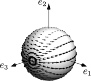
Here the Ωi​j\Omega_{ij} are the angular derivatives xi∂j−xj∂ix_{i}\partial_{j}-x_{j}\partial_{i} depicted as vector fields in Figure 1.

Refer to caption
Refer to caption
Refer to caption
Figure 1: Angular derivatives Ωi​j\Omega_{ij}
Proof.

We may prove the proposition for Q∈Cc∞​(B)Q\in C^{\infty}_{c}(B) and then get the claim by approximating. Test functions are dense in Cc1​(B)C^{1}_{c}(B) and sup|f|+sup|∇f|≤C​‖f‖C1\sup\left\lvert f\right\rvert+\sup\left\lvert\nabla f\right\rvert\leq C\left\lVert f\right\rVert_{C^{1}}. By Proposition 2.1 in [RU2]

∂τ(τ4​π​τ2​∫|x−a|=τQ⁡(s)​𝑑σ​(x))=1−τ2​Q​((1−τ)​a)+14​π​∫|x−a|=τα⋅∇Q​(x)sin⁡ϕ​𝑑σ​(x),\partial_{\tau}\left(\frac{\tau}{4\pi\tau^{2}}\int_{\left\lvert x-a\right\rvert=\tau}Q(s)d\sigma(x)\right)=\frac{1-\tau}{2}Q\big((1-\tau)a\big)+\frac{1}{4\pi}\int_{\left\lvert x-a\right\rvert=\tau}\frac{\alpha\cdot\nabla Q(x)}{\sin\phi}d\sigma(x),

where α=α⁡(a,x)\alpha=\alpha(a,x) is a unit vector orthogonal to xx and ϕ\phi is the angle at the origin between xx and aa.

Refer to caption
Figure 2: Reparametrization of |x−a|=τ\left\lvert x-a\right\rvert=\tau

Let Ti​j=xi​ej−xj​eiT_{ij}=x_{i}e_{j}-x_{j}e_{i} so Ωi​j=Ti​j⋅∇\Omega_{ij}=T_{ij}\cdot\nabla. Then for any vector vv we have

v=∑i<j(v⋅Ti​j|x|)​Ti​j|x|+(v⋅x|x|)​x|x|.v=\sum_{i<j}\left(v\cdot\frac{T_{ij}}{\left\lvert x\right\rvert}\right)\frac{T_{ij}}{\left\lvert x\right\rvert}+\left(v\cdot\frac{x}{\left\lvert x\right\rvert}\right)\frac{x}{\left\lvert x\right\rvert}.

On |x−a|=τ\left\lvert x-a\right\rvert=\tau set v:=αv:=\alpha and then take the dot product with ∇Q​(x)\nabla Q(x). We get

|x|2​α⋅∇Q​(x)=∑i<j(α⋅Ti​j)​(Ti​j⋅∇Q)​(x)=∑i<j(α⋅Ti​j)​Ωi​j​Q​(x)\left\lvert x\right\rvert^{2}\alpha\cdot\nabla Q(x)=\sum_{i<j}(\alpha\cdot T_{ij})(T_{ij}\cdot\nabla Q)(x)=\sum_{i<j}(\alpha\cdot T_{ij})\Omega_{ij}Q(x)

since x⟂αx\perp\alpha. By the Cauchy-Schwarz inequality

|α⋅∇Q​(x)|≤|a||x|​∑i<j|Ωi​j​Q​(x)|\left\lvert\alpha\cdot\nabla Q(x)\right\rvert\leq\frac{\left\lvert a\right\rvert}{\left\lvert x\right\rvert}\sum_{i<j}\left\lvert\Omega_{ij}Q(x)\right\rvert

since |Ti​j|≤|x|\left\lvert T_{ij}\right\rvert\leq\left\lvert x\right\rvert. This implies

|E⁡(a,τ)|≤|a|4​π​∑i<j∫|x−a|=τ|Ωi​j​Q​(x)||x|​|sin⁡ϕ|​𝑑σ​(x).\left\lvert E(a,\tau)\right\rvert\leq\frac{\left\lvert a\right\rvert}{4\pi}\sum_{i<j}\int_{\left\lvert x-a\right\rvert=\tau}\frac{\left\lvert\Omega_{ij}Q(x)\right\rvert}{\left\lvert x\right\rvert\left\lvert\sin\phi\right\rvert}d\sigma(x).

The law of cosines gives us 2​|a|​|x|​cos⁡ϕ=|a|2+|x|2−τ22\left\lvert a\right\rvert\left\lvert x\right\rvert\cos\phi=\left\lvert a\right\rvert^{2}+\left\lvert x\right\rvert^{2}-\tau^{2}. Solve for cos⁡ϕ\cos\phi to get sin⁡ϕ=±1−cos2⁡ϕ\sin\phi=\pm\sqrt{1-\cos^{2}\phi} and hence

1|sin⁡ϕ|=2​|a|​|x|4​|a|2​|x|2−(|a|2+|x|2−τ2)2\displaystyle\frac{1}{\left\lvert\sin\phi\right\rvert}=\frac{2\left\lvert a\right\rvert\left\lvert x\right\rvert}{\sqrt{4\left\lvert a\right\rvert^{2}\left\lvert x\right\rvert^{2}-(\left\lvert a\right\rvert^{2}+\left\lvert x\right\rvert^{2}-\tau^{2})^{2}}}
=2​|a|​|x|(|x|−τ+|a|)​(|x|+τ−|a|)​(τ+|a|−|x|)​(τ+|a|+|x|).\displaystyle\qquad=\frac{2\left\lvert a\right\rvert\left\lvert x\right\rvert}{\sqrt{(\left\lvert x\right\rvert-\tau+\left\lvert a\right\rvert)(\left\lvert x\right\rvert+\tau-\left\lvert a\right\rvert)(\tau+\left\lvert a\right\rvert-\left\lvert x\right\rvert)(\tau+\left\lvert a\right\rvert+\left\lvert x\right\rvert)}}.

But note that by assumption |a|>τ>0\left\lvert a\right\rvert>\tau>0 and |a|>|x|\left\lvert a\right\rvert>\left\lvert x\right\rvert for all x∈Bx\in B. Hence

1|sin⁡ϕ|≤2​|a|​|x||a|−τ​|x|−(|a|−τ)​τ​|a|.\frac{1}{\left\lvert\sin\phi\right\rvert}\leq\frac{2\left\lvert a\right\rvert\left\lvert x\right\rvert}{\sqrt{\left\lvert a\right\rvert-\tau}\sqrt{\left\lvert x\right\rvert-(\left\lvert a\right\rvert-\tau)}\sqrt{\tau}\sqrt{\left\lvert a\right\rvert}}.

and we can continue with

|E⁡(a,τ)|≤|a|22​π​τ​|a|​|a|−τ​∑i<j∫|x−a|=τ|Ωi​j​Q​(x)||x|−(|a|−τ)​𝑑σ​(x).\left\lvert E(a,\tau)\right\rvert\leq\frac{\left\lvert a\right\rvert^{2}}{2\pi\sqrt{\tau\left\lvert a\right\rvert}\sqrt{\left\lvert a\right\rvert-\tau}}\sum_{i<j}\int_{\left\lvert x-a\right\rvert=\tau}\frac{\left\lvert\Omega_{ij}Q(x)\right\rvert}{\sqrt{\left\lvert x\right\rvert-(\left\lvert a\right\rvert-\tau)}}d\sigma(x).

Finally, use the Cauchy-Schwarz inequality twice: once for (∑i<jfi​j)2≤3​∑i<jfi​j2(\sum_{i<j}f_{ij})^{2}\leq 3\sum_{i<j}f_{ij}^{2} and a second time for the product of the two function |Ωi​j​Q​(x)|/(|x|−(|a|−τ))1/4\left\lvert\Omega_{ij}Q(x)\right\rvert/(\left\lvert x\right\rvert-(\left\lvert a\right\rvert-\tau))^{1/4} and (|x|−(|a|−τ))−1/4(\left\lvert x\right\rvert-(\left\lvert a\right\rvert-\tau))^{-1/4}. It gives

|E⁡(a,τ)|2≤3​|a|3​I​(a,τ)4​π2​τ​(|a|−τ)​∑i<j∫|x−a|=τ|Ωi​j​Q​(x)|2|x|−(|a|−τ)​𝑑σ​(x)\left\lvert E(a,\tau)\right\rvert^{2}\leq\frac{3\left\lvert a\right\rvert^{3}I(a,\tau)}{4\pi^{2}\tau(\left\lvert a\right\rvert-\tau)}\sum_{i<j}\int_{\left\lvert x-a\right\rvert=\tau}\frac{\left\lvert\Omega_{ij}Q(x)\right\rvert^{2}}{\sqrt{\left\lvert x\right\rvert-(\left\lvert a\right\rvert-\tau)}}d\sigma(x)

where I⁡(a,τ)=∫|x−a|=τ,|x|≤|a|d​σ​(x)/|x|−(|a|−τ)I(a,\tau)=\int_{\left\lvert x-a\right\rvert=\tau,\left\lvert x\right\rvert\leq\left\lvert a\right\rvert}d\sigma(x)/\sqrt{\left\lvert x\right\rvert-(\left\lvert a\right\rvert-\tau)}.

Parametrize the sphere |a−x|=τ\left\lvert a-x\right\rvert=\tau by ρ=|x|\rho=\left\lvert x\right\rvert and the azimuth θ∈[0,2​π]\theta\in{[{0,2\pi}]} to calculate I⁡(a,τ)I(a,\tau). The latter variable gives the inclination of the plane a​O​xaOx with respect to a fixed reference plane passing through OO and aa. See Figure 2. We also introduce the polar angle ξ\xi. Using the standard spherical coordinates ξ\xi, θ\theta we have

d​σ​(x)=τ2​sin⁡ξ​d​ξ​d​θ=τ2​sin⁡ξ​d​ξd​ρ​d​ρ​d​θ.d\sigma(x)=\tau^{2}\sin\xi d\xi d\theta=\tau^{2}\sin\xi\frac{d\xi}{d\rho}d\rho d\theta.

By the law of cosines |a|2+τ2−2​|a|​τ​cos⁡ξ=ρ2\left\lvert a\right\rvert^{2}+\tau^{2}-2\left\lvert a\right\rvert\tau\cos\xi=\rho^{2}. Solve for cos⁡ξ\cos\xi and differentiate this with respect to the variable ρ\rho. Note that a,τa,\tau are constants, but ξ=ξ⁡(ρ)\xi=\xi(\rho). We get

−sin⁡ξ​d​ξd​ρ=dd​ρ​cos⁡ξ=−ρ|a|​τ-\sin\xi\frac{d\xi}{d\rho}=\frac{d}{d\rho}\cos\xi=-\frac{\rho}{\left\lvert a\right\rvert\tau}

which implies that d​σ​(x)=τ​|a|−1​ρ​d​ρ​d​θd\sigma(x)=\tau\left\lvert a\right\rvert^{-1}\rho d\rho d\theta.

Thus, since QQ vanishes outside BB, we have

I⁡(a,τ)=∫02​π∫|a|−τ|a|τ​|a|−1​ρ​d​ρ​d​θρ−(|a|−τ)≤2​π​τ​∫0τd​ρρ=4​π​τ3/2≤4​π​τ​|a|.I(a,\tau)=\int_{0}^{2\pi}\int_{\left\lvert a\right\rvert-\tau}^{\left\lvert a\right\rvert}\frac{\tau\left\lvert a\right\rvert^{-1}\rho d\rho d\theta}{\sqrt{\rho-(\left\lvert a\right\rvert-\tau)}}\leq 2\pi\tau\int_{0}^{\tau}\frac{d\rho}{\sqrt{\rho}}=4\pi\tau^{3/2}\leq 4\pi\tau\sqrt{\left\lvert a\right\rvert}.

Finally use the fact that BB is the unit ball and thus |a|=1\left\lvert a\right\rvert=1 to conclude the claim. ∎

We are now ready to prove stability for point source backscattering.

Proof of Theorem 1.1.

Write U~a=U1a−U2a\tilde{U}^{a}=U_{1}^{a}-U_{2}^{a} and q~=q1−q2\tilde{q}=q_{1}-q_{2}. By the assumptions and Proposition 4.1 we have

τ​U~a​(a,2​τ)=τ32​π2​τ2​∫|x−a|=τq~​(x)​𝑑σ​(x)+∫|x−a|≤τq~​(x)​τ​k​(x,τ,a)​𝑑x\tau\tilde{U}^{a}(a,2\tau)=\frac{\tau}{32\pi^{2}\tau^{2}}\int_{\left\lvert x-a\right\rvert=\tau}\tilde{q}(x)d\sigma(x)+\int_{\left\lvert x-a\right\rvert\leq\tau}\tilde{q}(x)\tau k(x,\tau,a)dx

for any τ>0\tau>0, in particular for h<τ<1h<\tau<1 which we shall assume now. By Proposition 4.2 and the differentiation formula for moving regions (e.g. [Evans] Appendix C.4) we get

∂τ(τ​U~a​(a,2​τ))=1−τ8​q~​((1−τ)​a)+14​E​(a,τ)\displaystyle\partial_{\tau}\left(\tau\tilde{U}^{a}(a,2\tau)\right)=\frac{1-\tau}{8}\tilde{q}\big((1-\tau)a\big)+\frac{1}{4}E(a,\tau)
+∫|x−a|=τq~(x)τk(x,t,a)dσ(x)+∫|x−a|≤τq~(x)∂τ(τk(x,τ,a))dx.\displaystyle\qquad+\int_{\left\lvert x-a\right\rvert=\tau}\tilde{q}(x)\tau k(x,t,a)d\sigma(x)+\int_{\left\lvert x-a\right\rvert\leq\tau}\tilde{q}(x)\partial_{\tau}(\tau k(x,\tau,a))dx.

By the Cauchy–Schwarz inequalities of ℝ4\mathbb{R}^{4} and the L2L^{2}-based function spaces L2({|x−a|=τ})L^{2}(\{\left\lvert x-a\right\rvert=\tau\}) and L2({|x−a|≤τ})L^{2}(\{\left\lvert x-a\right\rvert\leq\tau\}) we have

(1−τ)2​|q~​((1−τ)​a)|2≤256​|∂τ(τ​U~a​(a,2​τ))|2+16​|E⁡(a,τ)|2\displaystyle(1-\tau)^{2}\left\lvert\tilde{q}\big((1-\tau)a\big)\right\rvert^{2}\leq 256\left\lvert\partial_{\tau}\left(\tau\tilde{U}^{a}(a,2\tau)\right)\right\rvert^{2}+16\left\lvert E(a,\tau)\right\rvert^{2}
+256∫|x−a|=τ|q~(x)|2dσ(x)∫supp⁡q~∩|x−a|=τ|τk(x,τ,a)|2dσ(x)\displaystyle\qquad+256\int_{\left\lvert x-a\right\rvert=\tau}\left\lvert\tilde{q}(x)\right\rvert^{2}d\sigma(x)\int_{\supp\tilde{q}\cap\left\lvert x-a\right\rvert=\tau}\left\lvert\tau k(x,\tau,a)\right\rvert^{2}d\sigma(x)
+256∫|x−a|≤τ|q~(x)|2dx∫supp⁡q~∩|x−a|≤τ|∂τ(τk(x,τ,a))|2dx\displaystyle\qquad+256\int_{\left\lvert x-a\right\rvert\leq\tau}\left\lvert\tilde{q}(x)\right\rvert^{2}dx\int_{\supp\tilde{q}\cap\left\lvert x-a\right\rvert\leq\tau}\left\lvert\partial_{\tau}(\tau k(x,\tau,a))\right\rvert^{2}dx

Note that q1​(x)=q2​(x)=0q_{1}(x)=q_{2}(x)=0 for |x−a|<h\left\lvert x-a\right\rvert<h. Also recall the estimates (24) and (25) for integrals of kk from Proposition 4.1. We can proceed then with

(1−τ)2​|q~​((1−τ)​a)|2≤CM,h,B​(|∂τ(τ​U~a​(a,2​τ))|2+|E⁡(a,τ)|2CLOSE\displaystyle(1-\tau)^{2}\left\lvert\tilde{q}\big((1-\tau)a\big)\right\rvert^{2}\leq C_{M,h,B}\Big(\left\lvert\partial_{\tau}\left(\tau\tilde{U}^{a}(a,2\tau)\right)\right\rvert^{2}+\left\lvert E(a,\tau)\right\rvert^{2}
+∫|x−a|=τ|q~(x)|2dσ(x)+∫|x−a|≤τ|q~(x)|2dx)\displaystyle\qquad+\int_{\left\lvert x-a\right\rvert=\tau}\left\lvert\tilde{q}(x)\right\rvert^{2}d\sigma(x)+\int_{\left\lvert x-a\right\rvert\leq\tau}\left\lvert\tilde{q}(x)\right\rvert^{2}dx\Big)

since ‖q1‖C7,‖q2‖C7≤ℳ{\left\lVert q_{1}\right\rVert_{C^{7}}},{\left\lVert q_{2}\right\rVert_{C^{7}}}\leq\mathcal{M}.

Integrate the above estimate with ∫a∈∂B…​𝑑σ​(a)\int_{a\in\partial B}\ldots d\sigma(a) and use the coordinate change of Lemma 5.1. Then write 𝒬⁡(r)=∫|x|=r|q~​(x)|2​𝑑σ​(x)\mathcal{Q}(r)=\int_{\left\lvert x\right\rvert=r}\left\lvert\tilde{q}(x)\right\rvert^{2}d\sigma(x) and scale the integration variable on the left-hand side to get

𝒬⁡(1−τ)Cℳ,h,B≤∫|a|=1|∂τ(U~a​(a,2​τ))|2​𝑑σ​(a)+∫|a|=1|E⁡(a,τ)|2​𝑑σ​(a)\displaystyle\frac{\mathcal{Q}(1-\tau)}{C_{\mathcal{M},h,B}}\leq\int_{\left\lvert a\right\rvert=1}\left\lvert\partial_{\tau}(\tilde{U}^{a}(a,2\tau))\right\rvert^{2}d\sigma(a)+\int_{\left\lvert a\right\rvert=1}\left\lvert E(a,\tau)\right\rvert^{2}d\sigma(a)
+π∫|x|≥1−τ|q~(x)|2τ2+2​τ−(1−|x|)2|x|dx.\displaystyle\qquad\quad+\pi\int_{\left\lvert x\right\rvert\geq 1-\tau}\left\lvert\tilde{q}(x)\right\rvert^{2}\frac{\tau^{2}+2\tau-(1-\left\lvert x\right\rvert)^{2}}{\left\lvert x\right\rvert}dx. (27)

Next, estimate |E⁡(a,τ)|2\left\lvert E(a,\tau)\right\rvert^{2} using Proposition 4.2. Then change the order of integration using Lemma 5.1, switch to angular coordinates, and apply angular control (3) to get

∫|a|=1|E⁡(a,τ)|2​𝑑σ​(a)≤6​τ1−τ​∑i<j∫|x|≥1−τ|Ωi​j​q~​(x)||x|​|x|−(1−τ)​𝑑σ​(x)\displaystyle\int_{\left\lvert a\right\rvert=1}\left\lvert E(a,\tau)\right\rvert^{2}d\sigma(a)\leq\frac{6\tau}{1-\tau}\sum_{i<j}\int_{\left\lvert x\right\rvert\geq 1-\tau}\frac{\left\lvert\Omega_{ij}\tilde{q}(x)\right\rvert}{\left\lvert x\right\rvert\sqrt{\left\lvert x\right\rvert-(1-\tau)}}d\sigma(x)
=6​τ1−τ​∑i<j∫1−τ1∫|x|=r|Ωi​j​q~​(x)|r​r−(1−τ)​𝑑σ​(x)​𝑑r\displaystyle\qquad=\frac{6\tau}{1-\tau}\sum_{i<j}\int_{1-\tau}^{1}\int_{\left\lvert x\right\rvert=r}\frac{\left\lvert\Omega_{ij}\tilde{q}(x)\right\rvert}{r\sqrt{r-(1-\tau)}}d\sigma(x)dr
≤6​S2​∫1−τ1τ1−τ​𝒬⁡(r)r​r−(1−τ)​𝑑r.\displaystyle\qquad\leq 6S^{2}\int_{1-\tau}^{1}\frac{\tau}{1-\tau}\frac{\mathcal{Q}(r)}{r\sqrt{r-(1-\tau)}}dr. (28)

Similarly, the last term in (27) can be written as

…=π​∫1−τ1τ2+2​τ−(1−r)2r​𝒬​(r)​𝑑r.\ldots=\pi\int_{1-\tau}^{1}\frac{\tau^{2}+2\tau-(1-r)^{2}}{r}\mathcal{Q}(r)dr. (29)

Finally, combine estimates (28) and (29) to change (27) into

𝒬⁡(1−τ)≤Cℳ,h,B​∫|a|=1|∂τ(τ​U~a​(a,2​τ))|2​𝑑σ​(a)\displaystyle\mathcal{Q}(1-\tau)\leq C_{\mathcal{M},h,B}\int_{\left\lvert a\right\rvert=1}\left\lvert\partial_{\tau}(\tau\tilde{U}^{a}(a,2\tau))\right\rvert^{2}d\sigma(a)
+Cℳ,h,B∫1−τ1(6​S2​τ(1−τ)​r​r−(1−τ)+πτ2+2​τ−(1−r)2r)𝒬(r)dr\displaystyle\qquad+C_{\mathcal{M},h,B}\int_{1-\tau}^{1}\left(\frac{6S^{2}\tau}{(1-\tau)r\sqrt{r-(1-\tau)}}+\pi\frac{\tau^{2}+2\tau-(1-r)^{2}}{r}\right)\mathcal{Q}(r)dr

which is valid for 0<τ<10<\tau<1.

Our next step is to prepare for Grönwall’s inequality. The inequality above can be written as

φ⁡(τ)≤d⁡(τ)+∫0τβ⁡(τ,s)​φ​(s)​𝑑s\varphi(\tau)\leq d(\tau)+\int_{0}^{\tau}\beta(\tau,s)\varphi(s)ds (30)

for 0<τ<10<\tau<1 where

φ⁡(τ)=𝒬⁡(1−τ),d⁡(τ)=Cℳ,h,B​∫|a|=1|∂τ(τ​U~a​(a,2​τ))|2​𝑑σ​(a)\varphi(\tau)=\mathcal{Q}(1-\tau),\qquad d(\tau)=C_{\mathcal{M},h,B}\int_{\left\lvert a\right\rvert=1}\left\lvert\partial_{\tau}(\tau\tilde{U}^{a}(a,2\tau))\right\rvert^{2}d\sigma(a)

and

β⁡(τ,s)=Cℳ,h,B​(6​S2​τ(1−τ)​(1−s)​τ−s+π​τ2+2​τ−s21−s).\beta(\tau,s)=C_{\mathcal{M},h,B}\left(\frac{6S^{2}\tau}{(1-\tau)(1-s)\sqrt{\tau-s}}+\pi\frac{\tau^{2}+2\tau-s^{2}}{1-s}\right).

Because of the singularities of β\beta we restrict (30) to 0<τ≤1−ε0<\tau\leq 1-\varepsilon for any given ε>0\varepsilon>0. We have 1−s≥1−τ≥ε>01-s\geq 1-\tau\geq\varepsilon>0 and τ≤1\tau\leq 1. In this situation we see easily that

β⁡(τ,s)≤6​Cℳ,h,B​S2ε2​τ−s+3​π​Cℳ,h,Bε​τ−s≤6​S2+3​πε2​Cℳ,h,Bτ−s.\beta(\tau,s)\leq\frac{6C_{\mathcal{M},h,B}S^{2}}{\varepsilon^{2}\sqrt{\tau-s}}+\frac{3\pi C_{\mathcal{M},h,B}}{\sqrt{\varepsilon}\sqrt{\tau-s}}\leq\frac{6S^{2}+3\pi}{\varepsilon^{2}}\frac{C_{\mathcal{M},h,B}}{\sqrt{\tau-s}}.

Denote CS,ℳ,h,B=(6​S2+3​π)​Cℳ,h,BC_{S,\mathcal{M},h,B}=(6S^{2}+3\pi)C_{\mathcal{M},h,B}.

An application of Grönwall’s inequality (Lemma 5.2) implies

φ⁡(τ)≤(1+2​CS,ℳ,h,B​ε−2)​sup0<τ0<1d⁡(τ0)​exp⁡(4​CS,ℳ,h,B2​ε−4​τ)\varphi(\tau)\leq\left(1+2C_{S,\mathcal{M},h,B}\varepsilon^{-2}\right)\sup_{0<\tau_{0}<1}d(\tau_{0})\exp\left(4C_{S,\mathcal{M},h,B}^{2}\varepsilon^{-4}\tau\right) (31)

for 0<τ≤1−ε0<\tau\leq 1-\varepsilon. Now, given any τ∈(0,1)\tau\in(0,1) we choose ε>0\varepsilon>0 such that τ≤1−ε\tau\leq 1-\varepsilon and the right-hand side of the estimate above is minimized. These conditions are satisfied for ε=1−τ\varepsilon=1-\tau. The claim (4) follows after recalling that φ⁡(τ)=∫|x|=1−τ|(q1−q2)​(x)|2​𝑑σ​(x)\varphi(\tau)=\int_{\left\lvert x\right\rvert=1-\tau}\left\lvert(q_{1}-q_{2})(x)\right\rvert^{2}d\sigma(x) and applying simple estimates.

Let us prove the norm estimate for q~=q1−q2\tilde{q}=q_{1}-q_{2} over the whole BB next. Rewrite (4) as

‖q~‖L2({|x|=r})≤Λeℭ/r4\left\lVert\tilde{q}\right\rVert_{L^{2}(\{\left\lvert x\right\rvert=r\})}\leq\Lambda e^{\mathfrak{C}/r^{4}}

where Λ=‖U1a−U2a‖\Lambda=\left\lVert U_{1}^{a}-U_{2}^{a}\right\rVert. Since Cc7​(B)↪W1,∞​(B){C^{7}_{c}(B)}\hookrightarrow W^{1,\infty}(B) and the potentials are supported in BB we have the Lipschitz-norm estimate |q~​(x)|≤|q~​(x+ℓ​x|x|)|+2​ℓ​ℳ\left\lvert\tilde{q}(x)\right\rvert\leq\lvert{\tilde{q}(x+\ell\frac{x}{\left\lvert x\right\rvert})\rvert}+2\ell\mathcal{M} for any ℓ≥0\ell\geq 0. Integration gives

‖q~‖L2({|x|=r})≤24​πℳrℓ+rr+ℓΛeℭ/(r+ℓ)4\left\lVert\tilde{q}\right\rVert_{L^{2}(\{\left\lvert x\right\rvert=r\})}\leq 2\sqrt{4\pi}\mathcal{M}r\ell+\frac{r}{r+\ell}\Lambda e^{\mathfrak{C}/(r+\ell)^{4}}

which we can estimate to

‖q~‖L2({|x|=r})≤24​πℳℓ+Λeℭ/ℓ4\left\lVert\tilde{q}\right\rVert_{L^{2}(\{\left\lvert x\right\rvert=r\})}\leq 2\sqrt{4\pi}\mathcal{M}\ell+\Lambda e^{\mathfrak{C}/\ell^{4}}

because 0≤r≤10\leq r\leq 1 and ℓ≥0\ell\geq 0. The full domain estimate (5) follows from Lemma 5.3.

The proof for q1−q2q_{1}-q_{2} radially symmetric proceeds as above until (30). Since in the condition of angular control (3) we can assume that S=0S=0, we have

β⁡(τ,s)=Cℳ,h,B​π​τ2+2​τ−s21−s≤Cℳ,h,B′1−s\beta(\tau,s)=C_{\mathcal{M},h,B}\pi\frac{\tau^{2}+2\tau-s^{2}}{1-s}\leq\frac{C^{\prime}_{\mathcal{M},h,B}}{1-s}

and so

φ⁡(τ)Cℳ,h,B′′≤‖U1a−U2a‖2+∫0τφ⁡(s)1−s​𝑑s.\frac{\varphi(\tau)}{C^{\prime\prime}_{\mathcal{M},h,B}}\leq\left\lVert U_{1}^{a}-U_{2}^{a}\right\rVert^{2}+\int_{0}^{\tau}\frac{\varphi(s)}{1-s}ds.

This type of integral inequality implies

φ⁡(τ)≤Cℳ,h,B′′​‖U1a−U2a‖2​exp⁡(∫0τCℳ,h,B′′1−s​𝑑s)\displaystyle\varphi(\tau)\leq C^{\prime\prime}_{\mathcal{M},h,B}\left\lVert U_{1}^{a}-U_{2}^{a}\right\rVert^{2}\exp\left(\int_{0}^{\tau}\frac{C^{\prime\prime}_{\mathcal{M},h,B}}{1-s}ds\right)
=Cℳ,h,B′′​‖U1a−U2a‖2​(1−τ)−2​α\displaystyle\qquad=C^{\prime\prime}_{\mathcal{M},h,B}\left\lVert U_{1}^{a}-U_{2}^{a}\right\rVert^{2}(1-\tau)^{-2\alpha}

for some α=α⁡(ℳ,h,B)\alpha=\alpha(\mathcal{M},h,B) by Grönwall’s inequality. Note that here τ\tau is allowed to be anywhere in the whole interval (0,1)(0,1) without any of the constants blowing up. Following the rest of the proof implies Hölder stability. ∎

5 Technical tools

We collect here some basic calculations and some well known theorems so that we may refer to them without losing focus in the main proof.

Lemma 5.1.

Let ff be a continuous function vanishing outside of BB and let τ<1\tau<1 positive. Then

∫|a|=1∫|x−a|=τf⁡(x)​𝑑σ​(x)​𝑑σ​(a)=2​π​τ​∫|x|≥1−τf⁡(x)|x|​𝑑x\int_{\left\lvert a\right\rvert=1}\int_{\left\lvert x-a\right\rvert=\tau}f(x)d\sigma(x)d\sigma(a)=2\pi\tau\int_{\left\lvert x\right\rvert\geq 1-\tau}\frac{f(x)}{\left\lvert x\right\rvert}dx

and

∫|a|=1∫|x−a|≤τf⁡(x)​𝑑x​𝑑σ​(a)=π​∫|x|≥1−τf⁡(x)|x|​(τ2−(1−|x|)2)​𝑑x.\int_{\left\lvert a\right\rvert=1}\int_{\left\lvert x-a\right\rvert\leq\tau}f(x)dxd\sigma(a)=\pi\int_{\left\lvert x\right\rvert\geq 1-\tau}\frac{f(x)}{\left\lvert x\right\rvert}\big(\tau^{2}-(1-\left\lvert x\right\rvert)^{2}\big)dx.
Proof.

The first equation was proven just before formula (2.10) in [RU2]. The left-hand side of the second equation was shown to be equal to

∫|x|≤1f⁡(x)​∫|a|=1H⁡(τ2−|x−a|2)​𝑑σ​(a)​𝑑x\int_{\left\lvert x\right\rvert\leq 1}f(x)\int_{\left\lvert a\right\rvert=1}H(\tau^{2}-\left\lvert x-a\right\rvert^{2})d\sigma(a)dx

therein too.

The last equality follows by noting that the integral of the Heaviside function is just the area of the spherical cap arising from the intersection of |a|=1\left\lvert a\right\rvert=1 and |a−x|=τ\left\lvert a-x\right\rvert=\tau. If |x|<1−τ\left\lvert x\right\rvert<1-\tau then this intersection is empty. Otherwise the area is seen to be 2​π⋅r⋅h2\pi\cdot r\cdot h, where r=1r=1 is the radius of the sphere {|a|=1}\{\left\lvert a\right\rvert=1\} and hh is the height of the cap along the ray y​0¯y\bar{0}. Two applications of Pythagoras’ theorem and some simple algebra imply that h=(τ2−(1−|x|)2)/(2​|x|)h=(\tau^{2}-(1-\left\lvert x\right\rvert)^{2})/(2\left\lvert x\right\rvert) and thus the final equality is proven. ∎

Lemma 5.2.

Let b>ab>a and d:(a,b)→ℝd\colon(a,b)\to\mathbb{R} be bounded and measurable. Moreover let β:(τ,s)↦β⁡(τ,s)\beta\colon(\tau,s)\mapsto\beta(\tau,s) be measurable whenever τ,s∈(a,b)\tau,s\in(a,b) and s<τs<\tau. Moreover let it satisfy

β⁡(τ,s)≤Cτ−s\beta(\tau,s)\leq\frac{C}{\sqrt{\tau-s}}

for some C<∞C<\infty whenever s<τs<\tau.

If φ:(a,b)→ℝ\varphi\colon(a,b)\to\mathbb{R} is a non-negative integrable function that satisfies the integral inequality

φ⁡(τ)≤d⁡(τ)+∫aτβ⁡(τ,s)​φ​(s)​𝑑s\varphi(\tau)\leq d(\tau)+\int_{a}^{\tau}\beta(\tau,s)\varphi(s)ds (32)

for almost all τ∈(a,b)\tau\in(a,b), then

φ⁡(τ)≤(1+2​C​b−a)​supa<τ0<bd⁡(τ0)​e4​C2​τ.\varphi(\tau)\leq(1+2C\sqrt{b-a})\sup_{a<\tau_{0}<b}d(\tau_{0})e^{4C^{2}\tau}.
Proof.

First of all note that since φ≥0\varphi\geq 0, we may estimate β\beta from above in the integral, and see that the former satisfies

φ⁡(τ)≤d⁡(τ)+C​∫aτφ⁡(s)τ−s​𝑑s\varphi(\tau)\leq d(\tau)+C\int_{a}^{\tau}\frac{\varphi(s)}{\sqrt{\tau-s}}ds

for almost all τ\tau.

Next bootstrap the above by estimating φ\varphi inside the integral using that same inequality. Then

φ⁡(τ)≤d⁡(τ)+C​∫aτd⁡(s)τ−s​𝑑s+C2​∫aτ∫asφ⁡(s′)τ−s​s−s′​d​s′​𝑑s.\varphi(\tau)\leq d(\tau)+C\int_{a}^{\tau}\frac{d(s)}{\sqrt{\tau-s}}ds+C^{2}\int_{a}^{\tau}\int_{a}^{s}\frac{\varphi(s^{\prime})}{\sqrt{\tau-s}\sqrt{s-s^{\prime}}}ds^{\prime}ds.

The double integral is estimated as follows: ∫aτ∫as…​d​s′​𝑑s=∫aτ∫s′τ…​𝑑s​d​s′\int_{a}^{\tau}\int_{a}^{s}\ldots ds^{\prime}ds=\int_{a}^{\tau}\int_{s^{\prime}}^{\tau}\ldots dsds^{\prime}, and then we are left to estimate ∫s′τ𝑑s/τ−s​s−s′\int_{s^{\prime}}^{\tau}ds/\sqrt{\tau-s}\sqrt{s-s^{\prime}}. To do that split the interval (s′,τ)(s^{\prime},\tau) into two equal parts by the midpoint s=(τ+s′)/2s=(\tau+s^{\prime})/2. In the interval s∈(s′,(τ+s′)/2)s\in(s^{\prime},(\tau+s^{\prime})/2) we have 1/τ−s≤2/(τ−s′)1/\sqrt{\tau-s}\leq\sqrt{2/(\tau-s^{\prime})} and ∫s′(τ+s′)/2𝑑s/s−s′=2​(τ−s′)\int_{s^{\prime}}^{(\tau+s^{\prime})/2}ds/\sqrt{s-s^{\prime}}=\sqrt{2(\tau-s^{\prime})}. Their product is equal to 22. The same deduction works in the second interval. Hence

∫s′τd​sτ−s​s−s′≤4\int_{s^{\prime}}^{\tau}\frac{ds}{\sqrt{\tau-s}\sqrt{s-s^{\prime}}}\leq 4

indeed and

φ⁡(τ)≤d⁡(τ)+C​∫aτd⁡(s)τ−s​𝑑s+4​C2​∫aτφ⁡(s′)​d​s′\varphi(\tau)\leq d(\tau)+C\int_{a}^{\tau}\frac{d(s)}{\sqrt{\tau-s}}ds+4C^{2}\int_{a}^{\tau}\varphi(s^{\prime})ds^{\prime}

follows.

The first two terms above have an upper bound

(1+2​C​b−a)​supa<τ0<bd⁡(τ0)(1+2C\sqrt{b-a})\sup_{a<\tau_{0}<b}d(\tau_{0})

because ∫aτ𝑑s/τ−s=2​τ−a≤2​b−a\int_{a}^{\tau}ds/\sqrt{\tau-s}=2\sqrt{\tau-a}\leq 2\sqrt{b-a}. Grönwall’s inequality implies the final claim: If φ⁡(τ)≤C1+C2​∫0τφ⁡(s)​𝑑s\varphi(\tau)\leq C_{1}+C_{2}\int_{0}^{\tau}\varphi(s)ds for τ≥0\tau\geq 0 where φ≥0\varphi\geq 0 then φ⁡(τ)≤C1​exp⁡(C2​τ)\varphi(\tau)\leq C_{1}\exp(C_{2}\tau). This follows for example from Appendix B.2.j in [Evans] and some algebra. Note however that the integral form of Grönwall’s inequality in Appendix B.2.k of [Evans] is weaker than this one. ∎

Lemma 5.3.

Let f:ℝ+→ℝf\colon\mathbb{R}_{+}\to\mathbb{R} be a positive function satisfying

f⁡(ℓ)≤A​ℓ+Λ​eℭ/ℓ4f(\ell)\leq A\ell+\Lambda e^{\mathfrak{C}/\ell^{4}}

for some Λ<∞\Lambda<\infty and any ℓ\ell in its domain. Then if 0<Λ<e−10<\Lambda<e^{-1} we have

f⁡(ℓ0)≤A​(2​ℭ)1/4+2(ln⁡1Λ)1/4f(\ell_{0})\leq\frac{A(2\mathfrak{C})^{1/4}+2}{\left(\ln\frac{1}{\Lambda}\right)^{1/4}}

where ℓ04=ℭ/(ln⁡1Λ)\ell_{0}^{4}=\mathfrak{C}/(\ln\frac{1}{\sqrt{\Lambda}}). If Λ≥e−1\Lambda\geq e^{-1} then we have the linear estimate

f⁡(ℓ0)≤(A​ℭ1/4+1)​e​Λ.f(\ell_{0})\leq(A\mathfrak{C}^{1/4}+1)e\Lambda.

for ℓ04=ℭ\ell_{0}^{4}=\mathfrak{C}.

Proof.

Since Λ<e−1\Lambda<e^{-1} the choice of ℓ0\ell_{0} is proper. Moreover we see immediately that

f⁡(ℓ0)≤A​(2​ℭ)1/4(ln⁡1Λ)1/4+Λ.f(\ell_{0})\leq\frac{A(2\mathfrak{C})^{1/4}}{(\ln\frac{1}{\Lambda})^{1/4}}+\sqrt{\Lambda}.

Recall the elementary inequality ln⁡1a≤1b​a−b\ln\frac{1}{a}\leq\frac{1}{b}a^{-b} for b>0b>0 and 0<a<e−10<a<e^{-1}. Set b=2b=2 and a=Λa=\Lambda to see that

Λ≤2ln⁡1Λ≤2(ln⁡1Λ)1/4\sqrt{\Lambda}\leq\frac{2}{\ln\frac{1}{\Lambda}}\leq\frac{2}{(\ln\frac{1}{\Lambda})^{1/4}}

since ln⁡1Λ>1\ln\frac{1}{\Lambda}>1 then. The first claim follows. The second claim is elementary. ∎

The following is from personal communication with Rakesh.

Lemma 5.4.

Let p:ℝ→ℝp\colon\mathbb{R}\to\mathbb{R} be a measurable function. Then, given any time t≥0t\geq 0 and position x∈ℝnx\in\mathbb{R}^{n} with t≥|x|t\geq\left\lvert x\right\rvert, we have

|y|+|x−y|≤t⟺(t−|y|)2−|x−y|2≥0\left\lvert y\right\rvert+\left\lvert x-y\right\rvert\leq t\quad\Longleftrightarrow\quad(t-\left\lvert y\right\rvert)^{2}-\left\lvert x-y\right\rvert^{2}\geq 0

and

∫|y|+|x−y|≤tp⁡((t−|y|)2−|x−y|2)|y|​𝑑y\displaystyle\int_{\left\lvert y\right\rvert+\left\lvert x-y\right\rvert\leq t}\frac{p\big((t-\left\lvert y\right\rvert)^{2}-\left\lvert x-y\right\rvert^{2}\big)}{\left\lvert y\right\rvert}dy
=∫|w|≤12​t2−|x|2p⁡((t2−|x|2−|w|)2−|w|2)|w|​𝑑w.\displaystyle\qquad=\int_{\left\lvert w\right\rvert\leq\frac{1}{2}\sqrt{t^{2}-\left\lvert x\right\rvert^{2}}}\frac{p\big((\sqrt{t^{2}-\left\lvert x\right\rvert^{2}}-\left\lvert w\right\rvert)^{2}-\left\lvert w\right\rvert^{2}\big)}{\left\lvert w\right\rvert}dw.
Proof.

The first claim follows from the triangle inequality applied to a triangle with vertices xx, yy and 0¯\bar{0}: t−|y|+|x−y|≥|x|−|y|+|x−y|≥0t-\left\lvert y\right\rvert+\left\lvert x-y\right\rvert\geq\left\lvert x\right\rvert-\left\lvert y\right\rvert+\left\lvert x-y\right\rvert\geq 0, so we may multiply the inequality

t−|y|−|x−y|≥0t-\left\lvert y\right\rvert-\left\lvert x-y\right\rvert\geq 0

by the former without changing sign.

Let p+​(r)=p​(r)p_{+}(r)=p(r) for r≥0r\geq 0 and p+​(r)=0p_{+}(r)=0 for r<0r<0. Denote the left-hand side integral in the statement by II. Then

I\displaystyle I =∫ℝ3p+​((t−|y|)2−|x−y|2)|y|​𝑑y\displaystyle=\int_{\mathbb{R}^{3}}\frac{p_{+}\big((t-\left\lvert y\right\rvert)^{2}-\left\lvert x-y\right\rvert^{2}\big)}{\left\lvert y\right\rvert}dy
=∫ℝ3∫−∞∞δ⁡(s−|y|)|y|​p+​((t−|y|)2−|x−y|2)​𝑑s​𝑑y\displaystyle=\int_{\mathbb{R}^{3}}\int_{-\infty}^{\infty}\frac{\delta(s-\left\lvert y\right\rvert)}{\left\lvert y\right\rvert}p_{+}\big((t-\left\lvert y\right\rvert)^{2}-\left\lvert x-y\right\rvert^{2}\big)dsdy
=∫−∞∞∫ℝ3δ⁡(s−|y|)|y|​p+​((t−|y|)2−|x−y|2)​𝑑y​𝑑s\displaystyle=\int_{-\infty}^{\infty}\int_{\mathbb{R}^{3}}\frac{\delta(s-\left\lvert y\right\rvert)}{\left\lvert y\right\rvert}p_{+}\big((t-\left\lvert y\right\rvert)^{2}-\left\lvert x-y\right\rvert^{2}\big)dyds
=2​∫−∞∞∫ℝ3δ⁡(s2−|y|2)​p+​((t−|y|)2−|x−y|2)​𝑑y​𝑑s.\displaystyle=2\int_{-\infty}^{\infty}\int_{\mathbb{R}^{3}}\delta(s^{2}-\left\lvert y\right\rvert^{2})p_{+}\big((t-\left\lvert y\right\rvert)^{2}-\left\lvert x-y\right\rvert^{2}\big)dyds.

Let L1:ℝ3→ℝ3L_{1}\colon\mathbb{R}^{3}\to\mathbb{R}^{3} be a rotation taking x↦(|x|,0,0)x\mapsto(\left\lvert x\right\rvert,0,0). Let it map y↦y′y\mapsto y^{\prime}. Then d​y=d​y′dy=dy^{\prime} and so

I=2​∫−∞∞∫ℝ3δ⁡(s2−|y′|2)​p+​((t−|y′|)2−|L1​x−y′|2)​d​y′​𝑑s.I=2\int_{-\infty}^{\infty}\int_{\mathbb{R}^{3}}\delta(s^{2}-\left\lvert y^{\prime}\right\rvert^{2})p_{+}\big((t-\left\lvert y^{\prime}\right\rvert)^{2}-\left\lvert L_{1}x-y^{\prime}\right\rvert^{2}\big)dy^{\prime}ds.

Next let (s,y′)↦z∈ℝ4(s,y^{\prime})\mapsto z\in\mathbb{R}^{4} be the Lorentz transformation given by

z0=t​s−|x|​y1′t2−|x|2,z1=t​y1′−|x|​st2−|x|2,z2=y2,z3=y3.z_{0}=\frac{ts-\left\lvert x\right\rvert y_{1}^{\prime}}{\sqrt{t^{2}-\left\lvert x\right\rvert^{2}}},\quad z_{1}=\frac{ty_{1}^{\prime}-\left\lvert x\right\rvert s}{\sqrt{t^{2}-\left\lvert x\right\rvert^{2}}},\quad z_{2}=y_{2},\quad z_{3}=y_{3}.

It is a trivial matter to see that d​z=d​y′​d​sdz=dy^{\prime}ds and the following identities

z02−z12=s2−y1′2,(t2−|x|−z0)2−z12=(t−s)2−(|x|−y1′)2.z_{0}^{2}-z_{1}^{2}=s^{2}-y_{1}^{\prime 2},\qquad\big(\sqrt{t^{2}-\left\lvert x\right\rvert}-z_{0}\big)^{2}-z_{1}^{2}=(t-s)^{2}-(\left\lvert x\right\rvert-y_{1}^{\prime})^{2}.

Finally, denoting |z|2=z12+z22+z32\left\lvert z\right\rvert^{2}=z_{1}^{2}+z_{2}^{2}+z_{3}^{2} and z⋅z=z02−|z|2z\cdot z=z_{0}^{2}-\left\lvert z\right\rvert^{2}, we have

I\displaystyle I =2​∫ℝ4δ⁡(z⋅z)​p+​((t2−|x|2−z0)2−|z|2)​𝑑z\displaystyle=2\int_{\mathbb{R}^{4}}\delta(z\cdot z)p_{+}\big((\sqrt{t^{2}-\left\lvert x\right\rvert^{2}}-z_{0})^{2}-\left\lvert z\right\rvert^{2}\big)dz
=∫−∞∞∫ℝ3δ⁡(z0−|z|)|z|​p+​((t2−|x|2−z0)2−|z|2)​d​z1​d​z2​d​z3​d​z0\displaystyle=\int_{-\infty}^{\infty}\int_{\mathbb{R}^{3}}\frac{\delta(z_{0}-\left\lvert z\right\rvert)}{\left\lvert z\right\rvert}p_{+}\big((\sqrt{t^{2}-\left\lvert x\right\rvert^{2}}-z_{0})^{2}-\left\lvert z\right\rvert^{2}\big)dz_{1}dz_{2}dz_{3}dz_{0}
=∫ℝ3p+​((t2−|x|2−|z|)2−|z|2)|z|​d​z1​d​z2​d​z3\displaystyle=\int_{\mathbb{R}^{3}}\frac{p_{+}\big((\sqrt{t^{2}-\left\lvert x\right\rvert^{2}}-\left\lvert z\right\rvert)^{2}-\left\lvert z\right\rvert^{2}\big)}{\left\lvert z\right\rvert}dz_{1}dz_{2}dz_{3}
=∫ℝ3p+​((t2−|x|2−|w|)2−|w|2)|w|​𝑑w\displaystyle=\int_{\mathbb{R}^{3}}\frac{p_{+}\big((\sqrt{t^{2}-\left\lvert x\right\rvert^{2}}-\left\lvert w\right\rvert)^{2}-\left\lvert w\right\rvert^{2}\big)}{\left\lvert w\right\rvert}dw

which implies the claim since (t2−|x|2−|w|)2−|w|2≥0(\sqrt{t^{2}-\left\lvert x\right\rvert^{2}}-\left\lvert w\right\rvert)^{2}-\left\lvert w\right\rvert^{2}\geq 0 if and only if t2−|x|2−|w|−|w|≥0\sqrt{t^{2}-\left\lvert x\right\rvert^{2}}-\left\lvert w\right\rvert-\left\lvert w\right\rvert\geq 0. ∎

Acknowledgements

I am indebted to Rakesh for the many discussions that led me to understanding the Goursat problem and how to show the well-posedness of the point source problem. Without his help this important part of the paper would have taken many more months to complete. In addition I would like to thank the anonymous referees and their comments. This led to the realization that radially symmetric potentials have a better stability estimate.

References

  • [Bal1] Balean, R.: The Null-Timelike Boundary Problem, University of New England, PhD thesis, 1996.
  • [Bal2] Balean, R.: The null-timelike boundary problem for the linear wave equation, Communications in Partial Differential Equations, 22 (1997), 1325–1360.
  • [Cag] Cagnac, F.: Problème de Cauchy sur un conoïde caractéristique pour des équations quasi-linéaires, Ann. Mat. Pura Appl. (4), 129 (1982), 13–41.
  • [Evans] Evans, L. C.: Partial Differential Equations, Graduate Studies in Mathematics, Vol 19, American Mathematical Society, Providence, Rhode Island, second edition, 2010.
  • [Fri] Friedlander, F. G.: The wave equation on a curved space-time, Cambridge University Press, February 1975.
  • [Man] Mandache, N.: Exponential instability in an inverse problem for the Schrödinger equation, Inverse Problems, 17, 5 (2001), 1435–1444.
  • [MU] Melrose, R. and Uhlmann, G.: Generalized Backscattering and the Lax-Phillips Transform, Serdica Math. J., 34 (2008), 1026–1044.
  • [RU1] Rakesh and Uhlmann, G.: Uniqueness for the inverse back-scattering problem for angularly controlled potentials, Inverse Problems, 30 (2014), 065005.
  • [RU2] Rakesh and Uhlmann, G.: The point source inverse back-scattering problem, Contemporary Mathematics, 644 (2015), 279–289.
  • [Rom] Romanov, V.: Integral Geometry and Inverse Problems for Hyperbolic Equations, Springer-Verlag Berlin Heidelberg, 1974.