Pairing properties from random distributions of single-particle energy levels
Abstract
Exploiting the similarity between the bunched single-particle energy levels of nuclei and of random distributions around the Fermi surface, pairing properties of the latter are calculated to establish statistically-based bounds on the basic characteristics of the pairing phenomenon. When the most probable values for the pairing gaps germane to the BCS formalism are used to calculate thermodynamic quantities, we find that while the ratio of the critical temperature to the zero-temperature pairing gap is close to its BCS Fermi gas value, the ratio of the superfluid to the normal phase specific heats at differs significantly from its Fermi gas counterpart. The largest deviations occur when a few levels lie closely on either side of the Fermi energy but other levels are far away from it. The influence of thermal fluctuations, expected to be large for systems of finite number of particles, were also investigated using a semiclassical treatment of fluctuations. When the average pairing gaps along with those differing by one standard deviations are used, the characteristic discontinuity of the specific heat at in the BCS formalism was transformed to a shoulder-like structure indicating the suppression of a second order phase transition as experimentally observed in nano-particles and several nuclei. Contrasting semiclassical and quantum treatments of fluctuations for the random spacing model is currently underway.
I Introduction
The pairing phenomenon is ubiquitous in systems of fermions interacting through attractive interactions. The development of the theory for electron pairing in solids by Bardeen-Cooper-Schriffer (BCS) [1, 2] was soon followed by the realization that pairing of neutrons and protons in nuclei led to gaps in their excitation energies [3]. Pairing also manifests itself in the binding energies of nuclei, even-even nuclei being slightly more bound than odd-even or odd-odd nuclei [4]. Level densities of excited nuclei [5, 6], their dynamical properties such as rotational inertia [7] and large amplitude motion in fissioning nuclei are also influenced by pairing [8]. Tunneling probabilities in spontaneously fissioning nuclei are enhanced owing to pairing and thermal neutrons induce fission of odd-A nuclei, e.g., vs . Pairing energies in nuclei receive contributions from sources besides BCS pairing as nuclear sizes are much smaller than the coherence length of the pairing field [9]. The odd-even staggering is caused by a combination of effects such as the pair-wise filling of orbitals, two- and three-body interactions, the bunching of single-particle levels near the Fermi energy, and the softness of nuclei to quadrupolar interactions. The global description of pairing in nuclei is based on the Hartree-Fock-Bogoliubov (HFB) scheme and its extensions [8, 10]. The attractive interactions between nucleons in the spin and channels are primarily responsible for pairing in nuclei. For accounts of recent developments in novel superfluids and superconductors in the condensed matter, nuclear and stellar environments, see Ref. [11].
Through measurements of nuclear level densities at closely spaced excitation energies , several attempts have been made to establish pairing correlations in nuclei [12, 13, 14, 15]. The critical temperature at which the pairing gaps vanish in systems of very large number of particles is a characteristic of a second order phase transition. will be hard to pin down in nuclei as they are comprised of small numbers of particles owing to significant fluctuations in the order parameter ), but distinct signatures can likely remain. The experimental procedure adopted has been to examine the behavior of the specific heat at constant volume vs (or vs ) inferred from using , and looking for a smooth, but non-monotonic structure in at a critical excitation energy (or remnant of a critical temperature “”) which signals a crossover from the fully paired to the normal phase. The moderate success achieved thus far is due to issues associated with the normalization of level densities close to the neutron separation energy [16]. From an experimental perspective, excitation energies are well known, but not the temperature (unlike in condensed matter experiments) which requires the help of theoretical models in which the relationship between vs is unambiguous, albeit model dependent. (Hereafter, we will drop the quotes in “” for simplicity, but it should be understood as referring to the temperature around which a non-monotonic structure in vs is present.) Additional complications arise for due to the role of collective effects which influence the magnitude of . Notwithstanding these difficulties, the goal of establishing in nuclei appears to be within reach through continuing innovations in experimental techniques and theoretical efforts. Indeed, a shoulder-like structure (also referred to as an S-shape structure, although a severe bending of one’s head is required to see the S in many cases) in vs has been experimentally observed for many nuclei [12, 13, 14, 15].
The study of fluctuations in the order parameter and the suppression of superconductivity/superfluidity in systems of small number of particles (nano-particles in modern parlance) in condensed matter physics [17, 18] predates similar efforts in nuclear physics [20, 19]. The inadequacy of the mean-field BCS formalism becomes apparent in situations when the mean level spacing of the single-particle (sp) energy levels . As these studies have revealed, the absence of a second order phase transition with a discontinuity in at is direct consequence of large fluctuations in . A study of the role of thermal fluctuations, albeit with a semiclassical treatment of fluctuations following Refs. [21, 20], is also undertaken in this work. This treatment goes beyond BCS insofar as the gauge (number) symmetry broken in the BCS approach is restored. A full quantum treatment of fluctuations is outside the scope of this work, but will be reported separately.
In this work, we introduce the random spacing (RS) model to study the pairing properties of a system consisting of a finite number of nucleons. The basic feature of the RS model is the randomly distributed (sp) energy levels around the Fermi surface to mimic the bunched shell-model orbitals in nuclei generated through the use of different underlying energy density functionals. Although reminiscent of the random matrix model, the RS model differs from it in that diagonalization of a random Hamiltonian matrix is bypassed. Insofar as many random realizations of the sp energy levels will be considered for a fixed number of particles, the use of different physically motivated energy density functionals leading to different disposition of the sp levels will be captured. The pairing properties of the RS model are explored in two distinct stages as outlined below.
In the first stage, the BCS formalism in which the most probable gap values are employed to calculate thermodynamic quantities such as the excitation energy, entropy and specific heat is used. The ensuing results are compared with the analytical results of the Fermi gas (FG) and constant spacing (CS) models as well those of select nuclei. In the second stage, the role of fluctuations is examined based on a semiclassical treatment of fluctuations reserving for a later study a fully quantum treatment of the same. As in the first stage, a comparison with results of the CS model and those of nuclei including fluctuations is made.
The organization of this paper is as follows. In Sec. II, the basic features of the RS model are introduced. A description of the theoretical approach in the first stage of our investigations and a discussion of our results is contained in Sec. III. The influence of thermal fluctuations on the pairing gap and on the thermodynamic quantities examined in the second stage is described in Sec. IV, which also includes results and discussion. Our summary and conclusions are in Sec. V.
II The Random Spacing Model
Our objective here is to examine the pairing properties in a global manner keeping in mind that the single-particle (sp) energies of nuclei exhibit bunching caused by shell and pairing effects. Figure 1 shows the bunching of neutron sp energies from HFB calculations using the energy density functional SkO′ with full pairing in 57Co, 126Sn and 197Pt [22, 23]. The proton levels for these cases (not shown) also exhibit similar bunching. We stress, however, that use of different energy density functionals and pairing schemes (constant force, surface or bulk pairing, etc.) lead to significant differences in the spacing of levels around the Fermi surface [24].

When the sp levels of a large number of nuclei are examined, they appear to resemble those generated randomly around the Fermi surface. An example is shown in Fig. 2 where the neutron sp levels of are contrasted with three cases of randomly generated sp levels with the same number of neutrons at . Although not exact replicas, the latter share the property of bunched levels with nuclei. In a set consisting of a very large number of randomly generated sp levels for a given nucleus, some are likely to represent the true situation, especially considering the dependence on different energy density functionals currently in use. Thus, the primary focus of this work is to examine the pairing properties from randomly distributed sp energy levels with appropriate constraints imposed to model sp energy levels of nuclei. We will (i) address the extent to which the basic characteristics such as (where ), the ratio of superfluid to normal specific heats at constant volume, and compare with those Fermi gas (FG) and HFB calculations, and (ii) place statistically-based bounds for the case randomly distributed sp energy levels.

III Pairing Properties
With model sp energies as input, various physical quantities can be calculated utilizing the BCS equations generalized to include angular momentum [25]:
| (1) | |||||
| (2) | |||||
| (3) |
where denotes the number of particles, are the sp energies, is the chemical potential, and is the temperature. The summation index takes on the values 1 and 2, whereas the index sums over all sp energy levels. The quasi-particle energy is
| (4) |
where is the pairing gap at the Fermi surface generated by the pairing interaction with strength . The quantity is the projection of the total angular momentum on a laboratory-fixed -axis or on a body-fixed -axis, are the sp spin projections and is the Lagrange multiplier that fixes . Equations (1)-(3), studied as a function of for fixed provide the critical temperature below which the system is paired and above which it is normal . The excitation energy , entropy and the specific heat at constant volume are obtained from [25, 26]
| (5) | |||||
| (7) |
where .
To mimic the sp energy levels of nuclei in the random spacing (RS) model, random numbers from a uniform sequence are generated between from the Fermi energy ) with , where is the mass number, to conform to the systematics of spacing between major shells in nuclei [4]. For light nuclei, Ref. [27] recommends the relation . HFB and/or HF+BCS calculations of nuclei guide the choice of in solving Eqs. (1) and (2) to obtain and . In the results reported below, the pairing energies were tallied with the systematics for nuclei with [28]. For the neutron pairing gaps,
| (8) |
whereas for the proton pairing gaps,
| (9) |
As in the case of the FG or constant spacing (CS) models, an analytical calculation of [2, 26] is precluded for discrete bunched levels. We have therefore devised a 3-term formula utilizing Refs. [29, 30] to calculate . Explicitly, for a general and step size , the right end-point derivative is
| (10) |
Results
First, we recall the analytical results for spin-doublet sp levels (degeneracy ) in the FG model in which the sp level density and for the CS model in which is a constant, for both of which [1, 2, 25, 26, 31]
| (11) | |||||
where are the upper and lower limits of integration above and below the Fermi energy . The similarity of results in these two models stems from the conditions , (i.e., pairing is a Fermi surface phenomenon) and (weak coupling) being satisfied.
Our results for the RS model are for a large number () of independent random realizations of sp energy levels for a given at . The pairing gap vs shown in Fig. 3(a) corresponds to 500 such realizations with , and (similar results ensue for other values of ) for spin-doublet levels. The varying and are due to the different set of sp levels encountered in each run. Every curve in this figure resembles the BCS prediction for the FG or CS model. The nearly universal behavior displayed in Fig. 3(b) indicates that even for randomly generated sp levels, deviations from the BCS relations
| (13) | |||||
are small. Small quantitative differences from the BCS result for intermediate values of , evident from the band-like structure of the bell-shaped curve in Fig. 3(b), are caused by the variety of levels close to .


The ratio at is shown in Fig. 4. Note that the scatter around the mean value, which is moderately close to that for the FG or CS model, is significant for the RS model. The outlying points in this figure correspond to cases in which a couple of levels lie closely on either side of , but other levels are far away from it. In Table 1, the basic characteristics of the phase transition for the RS model are compared with those of FG and CS models.


| Model | Q= - | ||
|---|---|---|---|
| FG & CS() | |||
| CS() | |||
| RS() | |||
| RS() | |||
| HF+BCS(57Co) | 0.59,0.56 | 2.30,2.33 | 9.85,9.75 |
| HF+BCS(126Sn) | N/A,0.54 | N/A,4.47 | N/A,10.03 |
| HF+BCS(197Pt) | 0.55,0.54 | 3.46,4.93 | 10.33,10.52 |
The role of angular momentum on is shown in Fig. 5 for the RS model with MeV and to provide comparison with similar results for the CS model [25]. Increasing values of and diminish , and thus relative to when . As for the CS model, the paired region extends to beyond at which in the RS model with in accord with for the former case. For , two critical points exist in both of these models. For values of accessible in experiments, this region is likely not encountered. We have verified that up to , the first order approximation, , is sufficiently accurate, terms involving higher even powers of being required only for larger .
Endowing the sp energy levels of the CS and RS models with angular momentum degeneracies of the shell model orbitals of spherical nuclei yield results similar (to within the standard deviations shown in Table 1) to those for nuclei. The results for the nuclei shown conform to the nuclear systematics in Eq. (8). Results of the RS model for values of other than 76 show similar trends. For example, , and for . Note that although ’s remain close to the FG or CS model predictions, properties associated with the specific heat vary considerably in the RS model as well as in HF+BCS calculations owing to the variety of bunched sp levels encountered. The largest deviations from the mean values occur when a few levels are on either side of , but other levels are far away from it (see Fig. 6). In such cases, is significantly smaller than those in other cases which renders the ratio very large.

Unlike in the FG and CS models in which the parameter chiefly determines the pairing properties, the average density of states and separately influence results in the RS model as well as those in HF+BCS calculations of nuclei. By comparing with results of HFB calculations for typical cases, we have verified that results of the RS model encompass the case of deformed nuclei for which the above degeneracies are lifted.
IV Influence of Fluctuations in
The gap equation, Eq. (2), follows from the condition
| (14) |
where (we take hereafter for simplicity) the function
| (15) | |||||
determines the grand partition function . Equation (14) delivers the most probable gap values . The transition to the paired state is usually a second order phase transition and is its order parameter. Its decrease with increasing is continuous with a discontinuity in its slope at the critical temperature beyond which the system becomes unpaired. There is no latent heat but a discontinuity in specific heat at . Utilizing to determine the thermal variables is justified when the corresponding probability distribution is sharply peaked at . In a system with a large number of particles, approaches a delta function. However, nuclei are comprised of a small number of particles and fluctuations can be very large, particularly when the mean single-particle level spacing . In this case, superconductivity/superfluidity is expected to vanish although pairing correlations may persist. For small number of particles, but still with , quantum fluctuations suppress superconducting properties and the mean field BCS theory becomes invalid. These features were uncovered for small superconducting grains (nano particles) in condensed matter physics [17, 18] and are also characteristic of nuclei with small number of particles [19].
When and can be considered as strongly coupled to all the other intrinsic degrees of freedom, the isothermal semiclassical probability distribution for is given by [21, 20]
| (16) |
As emphasized in Ref. [21], when the temperature is too low or when varies too rapidly with time the fluctuations cannot be treated thermodynamically, and a quantum treatment becomes necessary to account for the purely quantum fluctuations. Here we will use the semiclassical treatment of fluctuations in as in Ref. [20] by using Eq. (16) to examine the extent of its utility and also to identify the regions of or in which a proper quantum treatment is necessary.
In what follows, we consider the role of fluctuations in on the thermal variables for the CS, RS and HFB models when the gap values
| (17) |
are used to calculate the various thermal variables. For any value of including , the number, energy, and entropy expressions (for ) ) are given by [25, 20]
| (18) | |||||
where ,
| (19) | |||||
and
For , the familiar forms for these quantities are recovered as the factor in the last parenthesis in each of the above expressions is the gap equation in Eq. (2) for which vanishes. The specific heat at constant volume is readily evaluated numerically (or from the lengthy analytical expression in [32]). The numerical results presented below for and are for and , respectively, where appropriate. Note, however, that
| (21) |
except when , that can be any of and , is a linear function of which is not true in the present context. Nonetheless, the results shown below amply illustrate the role of fluctuations in .
Note that the last terms in Eqs. (18) through () involving the gap equation together with appropriate multiplicative factors takes the semiclassical analysis of fluctuations beyond BCS, but remains at the mean field level insofar as only thermal fluctuations on a static underlying mean field are considered. Equation (18) ensures number conservation thereby restoring the broken gauge (number) symmetry of the BCS approach.
Results
The CS Model
Although the influence of fluctuations in the CS model have been considered before using the semiclassical treatment described above in Ref. [20], we summarize our main findings here to enable comparison with the results in the RS and HFB models to be discussed later. We also include results related with standard deviations from not shown in Ref. [20]. The role of fluctuations is analyzed by choosing a constant spacing between doubly degenerate single-particle levels for and at as in Ref. [20]. For this choice, MeV, MeV, with levels distributed between around MeV at . Figure 7 shows (normalized such that ) vs for different temperatures. Noteworthy features in this figure are: (i) For , the distribution is symmetrical around , (ii) with increasing , becomes increasingly asymmetrical, and (iii) For MeV, is peaked at .
Very similar results are obtained with (as in Ref. [20]) and for which MeV at MeV. In this case, the levels are distributed between to ensure that roughly equal number of levels lie above and below MeV. For all curves shown, vs is calculated using Eq. (18) prior to the calculation of required in the evaluation of in Eq. (16). The derivative needed in Eq. (18) is given by [25]
| (22) |
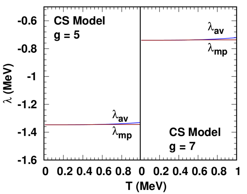
which is valid for all models and not just for the CS model. For , very nearly coincides with , whereas is slightly below for as shown in Fig. 8.

In Fig. 9, the most probable average paring gaps, and , vs are compared. Also shown are results for the standard deviation and the gaps . In each case, the appropriate was calculated with a numerical evaluation of the derivative . The discontinuity at that occurs for is absent for and . Furthermore, in the latter cases finite values of gaps persist for indicating that some high-energy quasi particles continue to undergo pairing. As first noted in Ref. [20], these results imply that the second order phase transition present for is considerably altered by fluctuations. We have verified that the qualitative features of these results are not changed when the degeneracy of each single-particle energy level is increased to 4 (for the same and ).

The excitation energies vs are shown in Fig. 10 for the various gap values shown in Fig. 9. The inset in Fig. 10 shows an expanded version of the same results in the vicinity of . Notice that the kink present in at is absent in all other cases as a consequence of smooth variations in ’s around at and around , further indicating the lack of a strong second order phase transition. The derivative , required in the evaluation from Eq. (19), is straightforwardly calculated numerically.


The influence of fluctuations in is particularly evident in the behavior of the specific heats, ’s, with respect to shown in Fig. 10 (b). Although the ’s with and exhibit multiple extrema, the sharp discontinuity of at is absent. Whether a similar behavior is exhibited in the RS and HFB models will be the subject of the next two subsections.
The RS Model
We turn now to examine the effects of fluctuations in for the RS model, first with degeneracy and thereafter to mimic shell-model-like configurations for . In both cases, the uniformly distributed random sp energy levels were sorted in ascending order. The mean level spacing , where is the mean level density, was chosen to be much smaller than MeV to facilitate a proper comparison with results of the CS model. For each set of random sp energy levels, the level separation and its probability distribution enables the calculation and thus of .
Degeneracy
The overall calculational scheme remains the same as for the CS model described above. Our results to be discussed below are for independent realizations of sp energy levels. The probability distribution vs in each case looks very similar to that of the CS Model in Fig. 7 and is therefore not shown.

Figure 11 shows the most probable gap and the average gap vs for independent realizations of sp energy levels. The standard deviations and were also calculated but are omitted for visual clarity. The band structures for and establish statistical bounds for each quantity. As for the CS model, lacks the sharp discontinuity at and persists with a non-vanishing gap above .


The excitation energies calculated using and from Eq. (19) are shown in Figs. 12(a) and (b), respectively. Particle number was conserved at every stage of the calculation by using the extended number equation Eq. (18). The kinks in at are absent in (Figs. 12 (a) and (b) ), again signifying the lack of a second order phase transition.


The corresponding specific heats, calculated by taking numerical derivatives, are shown in Figs. 13(a) and (b). The discontinuity in present for all different sets sp energy levels when using is absent when , likely more appropriate for systems with small number of particles for which fluctuations are large, is used. The discontinuity is replaced by a so-called “shoulder-like” structure, which points to the persistence of pairing correlations but not a second order phase transition. Note that the qualitative features for all thermodynamic quantities in the RS model with are similar to those of the CS Model.
Degeneracy
Inclusion of angular momentum degeneracy in the sp levels of the RS model makes the model to better mimic nuclei. In what follows, 36 sp energy levels were generated between using a uniform sequence random number generator and then sorted in ascending order so that the lowest energy level is at the bottom. The sorted energy levels were then assigned individual shell model-like degeneracies 2, 4, 6, etc. For each set of a large number of such realizations, the number and gap equations were then solved for and MeV for a fixed using the sp energy levels to extract the corresponding pairing strength and Fermi energy . To ensure pairing as a Fermi surface phenomenon, approximately equal number of energy levels are needed above and below the Fermi energy. Consequently, all the energy levels were then shifted by a constant energy so that the shifted Fermi energy is slightly below 0 MeV as a hole state.
The results of and for two such calculations as described above among hundreds of individual random realizations of sp energy levels are shown in Fig. 14. The latter two quantities were calculated following the procedure described at the beginning of this section. For the cases shown, the average level spacing was found to be and MeV, respectively, which are slightly less than the zero temperature gaps MeV. These numbers make a semiclassical treatment of fluctuations valid, albeit on the borderline of requiring a quantum treatment needed for cases in which as found for many nuclei. Note that the qualitative features in Fig. 14 are similar to those in Fig. 9 of the CS Model.

The excitation energies and specific heats corresponding to the results in Fig. 14 are shown in Fig. 15(a)-(d). Although the overall features in this figure seem very similar to those of the CS Model, values of and its slope with respect to ( are different owing to the different bunching and degeneracy of the individual sp energy levels of the RS model. As the number of particles in the two cases are fixed at , differences between the two cases reflect the different dispositions of the sp energy levels which can arise due to use of different energy density functionals in describing the same nucleus. One noticeable feature is that the curve calculated using - obtains slightly negative values for near zero temperatures. There is a possibility of similar occurrence even for for other sp energy realizations. This behavior can be attributed to the failure of a semiclassical treatment in the very low temperature region.


The specific heat curves in Figs. 15(c)-(d) again show the smoothing effect of fluctuations. The “shoulder-like” structures evident when fluctuations are incorporated as opposed to the sharp discontinuity in indicate the absence of a second order phase transition. This is a very close representation of the situation in nuclei as found in experiments.
HF calculations for Nuclei
In this section, results of HF calculations for the odd-even nucleus are compared with those of the CS and RS models. Pairing properties were calculated within the BCS formalism with a constant force for illustrative purposes. Neutrons and protons were treated as two separate systems, but owing to the linearity of thermodynamic quantities they can be simply added to obtain the same thermodynamic quantities for the whole nucleus. Figure 16 shows the proton and neutron gaps vs . The most probable gaps for protons and neutrons at were calculated by fixing the coupling strengths so that the gaps conform to the systematics indicated by Eqs. (8) and (9). Also shown are along with their standard deviations as a function of temperature. These results have qualitative resemblance with those of the CS and RS models.

The excitation energy and specific heat curves shown in Fig. 17 also show similar qualitative behavior to those of the RS Model. A noticeable feature is the larger fluctuations than for the RS Model. This is owing to being & MeV, respectively, for protons and neutrons. These values of are larger than the corresponding ’s which indicate that improvement over the mean field BCS treatment, which advocates use of most probable gaps, is necessary [17, 18, 21, 20, 19]. Results of our semiclassical treatment of fluctuations in the RS Model as well those in the HF+BCS calculations with a constant force highlights that pairing correlations persist even if a second order phase transition disappears. A similar semiclassical treatment of pairing correlations with similar results for using Nilson model sp energy levels can be found in Ref. [32]. Analogous results have been obtained with more advanced treatments that include improvements such as HFB calculations beyond mean field theory and a quantum treatment of fluctuations (see below and the many articles in Ref. [33]).


Detailed comparisons with experiments are premature at this development stage of the RS model. The influence of additional sources of fluctuations such as beyond mean field effects, collective effects and those from rotation should be considered in a fully quantum treatment to provide a comparison with the semiclassical treatment adopted in this work. We expect further modifications of the shoulder-like or the S-Shaped structure when these and additional sources of fluctuations are included.
Beyond mean field theory
The HF theory includes pairing in nuclei using the BCS approximation by treating the pair correlations through time-reversed orbital wave functions. In this approach, the HF equations are self-consistently solved to find variational minima using an underlying energy density functional. But the minima (HF wave functions) so obtained using HF/BCS could be different from that of HFB [8]. This is due to the more complete wave functions of the Bogoliubov transformation in contrast to the small configuration space HF wave functions. Hence, HFB is more inclusive of physical effects than HF.
In the HFB/BCS approach, broken symmetries which are artifacts of the mean field approximation appear. Beyond mean field techniques restore the number symmetry and treat fluctuations in the BCS order parameter; see Ref. [8] and references therein. Other popular techniques include the random phase approximation (RPA) and their derivatives [34]. Even then, many technical difficulties, such as the sign of the overlap of HFB wave functions and additional difficulties with odd-A nuclei, arise [8]. Correlations beyond the mean field have also been treated in Ref. [19] by using the Hubbard-Stratonovich (HS) transformation which can be incorporated in many different ways, e.g., the static-path approximation (SPA) in which only the thermal fluctuations are addressed. The SPA coupled with RPA includes time-dependent quantal fluctuations in addition to thermal effects. Advanced, but computationally intensive methods such as the Auxiliary-Field Monte Carlo (AFMC) approach include additional fluctuations [19]. This reference gives an account of the various methods employed to treat fluctuations at the quantum level.
While the static (BCS or HFB) mean field approximation is an adequate treatment for a spherical or non-rotating nucleus, dynamic effects (such as pairing vibrations) need to be included on top of the static mean field for a rotating nucleus. The effect of pairing on rapidly rotating nuclei is to significantly reduce the rigid body moment of inertia. The formation of Cooper pairs means having two nucleons with time-reversed conjugate orbits. In rapidly rotating nuclei, nucleons are forced to align their angular momenta with the rotation axis which leads to the breaking of Cooper pairs. This results in a gradual decrease of the effective pairing gap (static gap + dynamic gap) as opposed to a sharp disappearance of the static gap, see, e.g., [34].
In this work, we have examined the role of thermal fluctuations in the RS model using a semiclassical treatment. A quantitative comparison with a quantum treatment that includes additional sources of fluctuations within the RS model is beyond the scope of this paper, but will be reported in a separate work.
V Summary and Conclusions
We turn now to summary and conclusions. In the medium-to-heavy mass region, spherical and deformed nuclei accessible to laboratory experiments, and particularly those only realized in the highly neutron-rich environments encountered in astrophysical phenomena, are characterized by an assortment of bunched single-particle (sp) energy levels owing to shell and pairing effects. Laboratory experiments performed on various nuclei have revealed a shoulder-like structure around the critical temperature expected from a second order phase transition from the BCS formalism of the pairing phenomenon involving fermions, but not a discontinuous jump in the specific heat from the paired to the normal phase [12, 13, 14, 15].
The main contribution of this work is the introduction of the random spacing (RS) model in which the sp energy levels are distributed around the Fermi energy to mimic those of nuclei obtained via the use of different energy density functionals. The distributions of these sp energy levels closely resemble those of randomly generated levels around the Fermi surface. Exploiting this similarity, we have calculated the basic characteristics of the pairing correlations in the RS model and compared the results with those of select nuclei. Aspects of the RS model are studied in two distinct stages as summarized below.
In the first stage, the BCS formalism, which employs the most probable pairing gaps to calculate the critical temperature, the behaviors of the entropy and specific heat at constant volume as functions of temperature (excitation energy) and angular momentum, is used for the sp energy levels of the RS model. Comparisons with results of the Fermi gas, constant spacing models and nuclei are provided. Our principal results at this stage are as follows. From the statistically-based bounds obtained, we find that the ratio of the critical temperature to the zero-temperature pairing gap is close to its Fermi gas value, and appears to be a robust result. However, the ratio of the paired to normal phase specific heats at the critical temperature differs significantly from its Fermi gas counterpart. The scatter around the mean value for the discontinuity in the specific heat at the critical temperature is largest when a couple of sp levels lie closely on either side of the Fermi surface, but other levels are far away from it.
In the second stage, the role of fluctuations, expected to be large for systems with small number of particles, is studied. Based on a semiclassical treatment of thermal fluctuations first developed in Ref. [20] for the CS model and later applied with some improvements in Ref. [32] for , applications are considered here to the RS model. The chief result of this investigation is that the second order phase transition, a consequence of using the most probable values for the paring gaps in the BCS formalism, is suppressed and replaced by a shoulder-like structure around when the average values for the pairing gaps are used indicating the lasting presence of pairing correlations. Such a structure is indeed observed in experiments performed on several nuclei [12, 13, 14, 15]. We note, however, that a semiclassical treatment is strictly valid only when the mean sp level spacing around the Fermi surface is smaller or nearly equal to the zero temperature pairing gap and a fully quantum treatment of fluctuations becomes necessary otherwise to overcome the limitations of the BCS formalism [17, 18, 21, 20, 19]. Contrasting the semiclassical and quantum treatments of fluctuations as well as investigations of fluctuations in highly neutron-rich isotopes with more advanced techniques in the context of the RS model will be undertaken in future works.
To the extent that the sp levels of the RS model resemble those of nuclei that exhibit considerable dependence on choices of the energy density functionals and pairing schemes used, our results indicate the variation to be expected in the basic characteristics of the pairing phenomenon in nuclei. These results can help to perform sensitivity tests in astrophysical settings which harbor exotic nuclei.
acknowledgments
We thank P.-G. Reinhardt for providing us with computer programs to generate single-particle energy levels for nuclei based on various pairing schemes. Beneficial conversations with Steve Grimes, Alexander Voinov and Tom Massey are gratefully acknowledged. This work was performed with research support from the U.S. DOE grant No. DE-FG02-93ER-40756.
References
- [1] J. Bardeen, L. N. Cooper, and J. R. Schrieffer, Phys. Rev. 106, 162 (1957).
- [2] J. Bardeen, L. N. Cooper, and J. R. Schrieffer, Phys. Rev. 108, 1175 (1957).
- [3] A. Bohr, B. M. Mottelson, and D. Pines, Phys. Rev. 108, 936 (1958).
- [4] A. Bohr and B. R. Mottelson, Nuclear Structure, Vol. I: Single-Particle Motion (World Scientific Publishing, 1969).
- [5] H. A. Bethe, Phys. Rev. 50, 332 (1936).
- [6] T. Ericson, Adv. Phys. 9, 425 (1960).
- [7] A. Migdal, Nucl. Phys. A 13, 655 (1959).
- [8] L. M. Robledo and G. F. Bertsch, Pairing in finite systems: Beyond the HFB theory, in 50 years of Nuclear BCS: Pairing in Finite Systems, edited by R. A. Broglia and V. Zelevinsky, Singapore, 2013, World Scientific.
- [9] D. J. Dean and M. Hjorth-Jensen, Rev. Mod. Phys. 75, 607 (2003).
- [10] D. M. Brink and R. A. Broglia, Nuclear Superfluidity: Pairing in Finite Systems (Cambridge University Press, Cambridge, 2005).
- [11] K. H. Benneman and J. B. Ketterson, editors, Novel Superfluids, Vol. I and II (Oxford University Press, Oxford, 2015).
- [12] A. Schiller et al., Phys. Rev. C 63, 021306 (2001).
- [13] U. Agvaanluvsan et al., Phys. Rev. C 79, 014320 (2009).
- [14] H. K. Toft et al., Phys. Rev. C 81, 064311 (2010).
- [15] H. K. Toft et al., Phys. Rev. C 83, 044320 (2011).
- [16] M. Guttormsen, private communication.
- [17] P. W. Anderson, J. Phys. Chem. Solids 411, 26 (1959).
- [18] G. Falci, R. Fazio, F. W. J. Hekking, and A. Mastellone, Journal of Low Temperature Physics. 118, 355 (2000).
- [19] Y. Alhassid, Thermal signatures of pairing correlations in nuclei and metal nanoparticles, in 50 years of Nuclear BCS: Pairing in Finite Systems, edited by R. A. Broglia and V. Zelevinsky, p. 608, Singapore, 2013, World Scientific.
- [20] L. G. Moretto, Phys. Lett. B 185, 1 (1972).
- [21] L. D. Landau and E. M. Lifshitz, Statistical Physics Part 1 (Pergamon Press, Oxford, 1980).
- [22] K. Langanke, J. A. Maruhn, and S. E. Koonin, editors, Computational Nuclear Physics I (Springer-Verlag, London, UK, 1991), Chap. 2.
- [23] J. Friedrich and P.-G. Reinhard, Phys. Rev. C 33, 335 (1986).
- [24] P.-G. Reinhard et al., Phys. Rev. C 60, 014316 (1999).
- [25] L. G. Moretto, Nuclear Physics A 185, 145 (1972).
- [26] M. Sano and S. Yamasaki, Progr. Theor. Phys. 29, 397 (1963).
- [27] J. Blomquist and A. Molinari, Nucl. Phys. A106, 545 (1967).
- [28] G. F. Bertsch, Nuclear pairing: Basic phenomena revisited, in 50 years of Nuclear BCS: Pairing in Finite Systems, edited by R. A. Broglia and V. Zelevinsky, Singapore, 2013, World Scientific.
- [29] M. Abramowitz and I. A. Stegun, Handbook of Mathematical Functions, Applied Mathematical Series 55 (National Bureau of Standards, Washington D.C., 1972).
- [30] L. F. Richardson and J. A. Gaunt, Phil. Trans. R. Soc. A 226, 229 (1927).
- [31] E. M. Lifshitz and L. P. Pitaevskii, Statistical Physics Part 2 (Pergamon Press, Oxford, 1980).
- [32] Z. Kargar and V. Dehghani, J. Phys. G: Nucl. Part. Phys. 40, 045108 (2013).
- [33] R. A. Broglia and V. Zelevinsky, editors, 50 years of Nuclear BCS: Pairing in Finite Systems (World Scientific, Singapore, 2013).
- [34] Y. R. Shimizu, P. Donati, and R. A. Broglia, Phys. Rev. Lett. 85, 2260 (2000).