Deciphering the nonlocal entanglement entropy of fracton topological orders
Abstract
The ground states of topological orders condense extended objects and support topological excitations. This nontrivial property leads to nonzero topological entanglement entropy for conventional topological orders. Fracton topological order is an exotic class of models which is beyond the description of TQFT. With some assumptions about the condensates and the topological excitations, we derive a lower bound of the nonlocal entanglement entropy (a generalization of ). The lower bound applies to Abelian stabilizer models including conventional topological orders as well as type I and type II fracton models, and it could be used to distinguish them. For fracton models, the lower bound shows that could obtain geometry-dependent values, and is extensive for certain choices of subsystems, including some choices which always give zero for TQFT. The stability of the lower bound under local perturbations is discussed.
I Introduction
Topological order [1] is a gapped quantum phase of matter beyond the description of the Landau-Ginzburg theory of symmetry breaking. Many of the early examples of topological orders (which we will refer to as conventional topological orders) share the following properties: robust ground state degeneracy which depends on the topology of the manifold [1], the ground states are locally indistinguishable [1, 2, 3], the existence of integer dimensional condensates and logical operators that can be topologically deformed [4], nontrivial braiding statistics of anyons or other topological excitations (or topologically charged excitations) e.g., excitations which could not be created alone by local operators [5, 6], they are effectively described by topological quantum field theory (TQFT) at low temperatures [1], and they can be used to do fault-tolerant quantum information processing [7]. And it is well known that, in 2D, a suitable linear combination of entanglement entropy with local contributions canceled is a topological invariance called the topological entanglement entropy [8, 9]. Topological entanglement entropy is a property of the ground state wave function and it has been used to identify quantum spin liquid phases [10]. It also contains information about the ground state degeneracy [11] and the forms of low-energy excitations [12]. Generalizations of topological entanglement entropy into 3D bulk [13] and boundary [12] are studied.
On the other hand, there are recently discussed 3D exotic topological ordered models [14, 5, 15, 16, 17, 18, 19, 20, 21, 22, 23, 24] that do not fit very well into the pictures above. These models have recently been classified into fracton topological orders [18]. While fracton models have locally indistinguishable ground states when placed on nontrivial manifolds and the ground state degeneracy is robust under local perturbations [2, 3], the ground state degeneracy depends on the system size (geometry) rather than merely the topology of the manifold [5, 6, 16]. While fracton models possess topological excitations [5, 6], these topological excitations are constrained to move in lower dimensional submanifolds rather than the whole system [17, 18]. The condensates and logical operators can be fractal dimensional [16, 18] instead of integer dimensional. These models are beyond the description of TQFT.
There are type I and type II fracton topological orders. The type I fracton models include the Chamon-Bravyi-Leemhuis-Terhal (CBLT) model [14, 5], the Majorana cubic model [17], and the X-cube model [18], etc.; they have integer dimensional condensates and logical operators. The type II fracton models include Haah’s code [15] and many of the fractal spin liquid models [16] (see Sec.III.4). Type II fracton models possess fractal condensates and logical operators and the excitations are fully immobile [18].
For the ground state entanglement properties of fracton models, a relation to the ground state degeneracy is implied in [11] and the entanglement renormalization group transformation of Haah’s code is studied in [25]. In this work, we construct a direct analogy of topological entanglement entropy by doing linear combinations of entanglement entropies of different subsystems in such a way that the local contributions (from each boundary or corner of the subsystems) are canceled, and we call the linear combination , the nonlocal entanglement entropy. While is topologically invariant for conventional topological orders, it is geometry-dependent for fracton models.
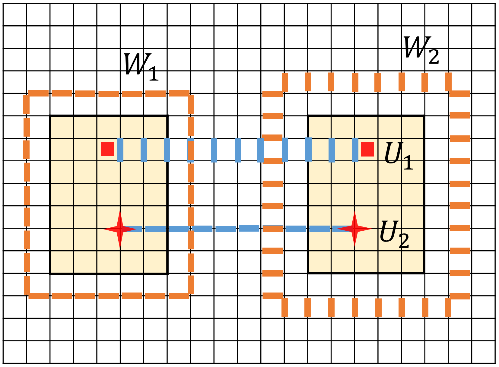
Explicitly, we choose a conditional mutual information form used by Kim and Brown [12] and define the nonlocal entanglement entropy . Where with being a ground state. The whole system is the union of subsystems , , , and with and separated by distance , the correlation length. One can check that the local contributions from the boundaries are canceled, and this is why we use the name “nonlocal entanglement entropy.” This construction can be used in any dimensions and an example in 2D is shown in Fig.1. With several assumptions about the condensates and topological excitations, a lower bound of is derived.
When applied to known conventional Abelian topological orders e.g. the 2D toric code model and the 3D toric code model [26], the lower bound is topologically invariant and it is identical to the exact result, i.e. the lower bound is saturated. When applied to fracton models [14, 5, 15, 16, 17, 18], the lower bound depends on the sizes and relative locations of the subsystems. For fracton models, there exist choices of subsystems for which the lower bound is nonzero and extensive. It is possible to have for subsystem choices, that are expected to have if TQFT holds.

This method observes an intimate relation between and topological excitations created in by a unitary operator stretched out in which could be “deformed” into a unitary operator in , and since deformable is intimately related to condensate operator (for more details of , and condensate operator see Sec.II.4), this method observes an intimate relation between and ground state condensates as well. This method allows a lower bound of to be obtained without calculating the entanglement entropy of any individual subsystem. Furthermore, it provides us with a unified viewpoint to understand the topology-dependent in the conventional topological orders and the geometry-dependent in fracton topological orders. Also discussed is the stability of the lower bound under local perturbations.
Two additional papers appeared after our work which also study the entanglement entropy of fracton phases, using explicit computation [27] and tensor network [28].
For non-Abelian models, some of our assumptions breakdown, and our original method does not apply. Nevertheless, a variant of our lower bound is applicable to non-Abelian models [29].
The structure of the paper is as follows: In Sec.II we provide a derivation of the lower bound from some assumptions about topological excitations and condensates; In Sec.III we apply our lower bound to several exactly solved Abelian stabilizer models of 2D, 3D conventional topological orders and type I, type II fracton topological orders. In Sec.IV we discuss the stability of the lower bound under local perturbations. Sec.V is discussion and outlook.
II The lower bound
II.1 A few notations and definitions
We will consider a infinite system without boundaries. The system is divided into subsystems , , , (nonoverlapping regions in real space, the union of which is the whole system). Each subsystem has a size large compared to the correlation length , and the subsystems and are separated by a distance much larger than the correlation length. One example is shown in Fig.1, and similar constructions can apply to any dimensions. For all the examples in this paper, we have chosen , , to be local subsystems while is not, but there exist other possible choices, say , , local. A local subsystem is a subsystem which can be contained in a ball-shaped subsystem of finite radius. , are the boundaries of the subsystems. We use to denote the complement of .
We will use , to represent density matrices. In this paper we always use for the ground state density matrix, , and is the ground state. We use , when we want to specify the subsystems. The entanglement entropy is defined in terms of the (reduced) density matrix as usual . We use and to distinguish the entanglement entropy on region with different density matrices , . Define conditional mutual information
and we use when we want to specify a density matrix. It is known that the conditional mutual information is always nonnegative . We say is conditionally independent if .
For unitary operators and which create excitations in when acting on the ground state , we say or is similar to if the states and have identical reduced density matrices on , i.e. . Otherwise, we say and are distinct.
II.2 Prepare for the lower bound
If there is a density matrix which is related to the ground state density matrix by and , then we have:
| (1) |
and the “” happens if and only if . For a proof, observe that and has only a single different term, and that .
For a pure state, the entanglement entropy of a subsystem equals the entanglement entropy of its complement, e.g. for any subsystem . Therefore:
Observe that the local contributions of the entanglement entropy get canceled due to the fact that and are separated. Let us define the nonlocal entanglement entropy (of the ground state)
| (2) |
The nonlocal entanglement entropy is just another way to write down the conditional mutual information, , and therefore . The form in Eq.(2) has the advantage that it involves only local systems , , . When the system is placed on a torus or other nontrivial manifolds instead of a infinite manifold, the system may have several locally indistinguishable ground states, this form of in terms of local subsystems is more convenient, and even if is a mixed state density matrix of different locally indistinguishable ground states, still has the same value.
II.3 The key idea about the lower bound
The discussion above suggests a way to obtain a lower bound of . For any satisfying and ,
| (3) |
The density matrix does not have to be a density matrix of a pure state. If we could find a satisfying the above requirement and , a nonzero lower bound is obtained, and then the existence of nonzero nonlocal entanglement entropy is established.
Now, let us assume that we could find a set of with such that and . Then we can do superpositions and define with being a probability distribution, i.e. and . The is a new density matrix which satisfies and . So we have a whole parameter space of to try.
If lucky, we may even be able to find a which is conditionally independent (satisfying ) and we have an exact result
| (4) |
Or, if we find the lower bound is saturated, we know the we used to obtain the lower bound is conditionally independent. We note that, in the quantum case (unlike the classical case), it is not always possible to find a conditionally independent such that and for being a general density matrix [30]. Therefore, the existence of such in some system might be interesting by itself. On the other hand, the conditional independent state is known to exist for models satisfying simple conditions (I)(II) in [31].
II.4 Calculate the lower bound for Abelian models employing assumptions
We make a few assumptions about the condensates and operators creating topological excitations in order to develop a way to find and calculate a lower bound of . These assumptions are applicable to Abelian models with commuting projector Hamiltonians (with each term acting on a few sites localized in real space), including conventional models e.g. the toric code model in various dimensions [26], quantum double models with any Abelian finite group, and fracton models [14, 5, 15, 16, 17, 18] of type I and type II which we will be focusing on in this work. In the context of fracton models, Abelian means no protected degeneracy associated with excitations.
Our way of employing the operators is inspired by a method by Kim and Brown [12], where an interesting connection between conditional mutual information and deformable operator is obtained. While the subsystems we choose have only an unimportant difference from [12], our result is different. The result in [12] shows that if , there will be no topological excitations, and therefore, is needed for the existence of topological excitations. The result is very general since very small amount of assumptions was used. Nevertheless, the result was not powerful as a lower bound for . In this work, on the other hand, we use more detailed properties of topological excitations and condensates to obtain a powerful lower bound of . Our method shows that the key to have in these models is the nonlocal nature of the ground state condensates and the operators creating topological excitations. can be extensive in the subsystem size and it is not necessarily topologically invariant. Whether is topologically invariant or not depends on whether the operators can be deformed topologically.

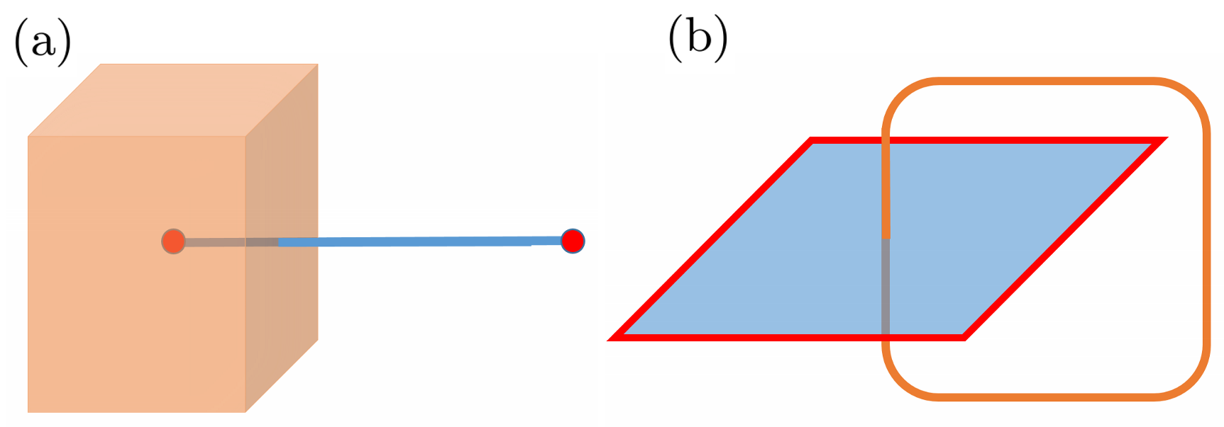
Before rigorously stating the assumptions and deriving the lower bound, here are a few words about the physical picture. The ground states of topological orders condense extended objects. If a unitary operator (which has an extended support) acting on the ground state gives you , we call the operator a condensate operator with eigenvalue . Whenever confusion can be avoided, we may call a condensate for short. Let us further assume to be a tensor product of operators acting on each site. Then, a suitably defined “truncation” of a condensate operator onto a subsystem gives you a new operator . is an excited state with topologically excitations located around , and can be deformed in the sense that you could choose a “truncation” of onto and call it , which creates the same topological excitations and satisfies . One the other hand, if we have unitary operators and satisfying , then , and therefore is a condensate operator with eigenvalue . Intuitively, a condensate operator can be “truncated” into a deformable operator which creates topological excitations, and a pair of deformable operators and can be “glued together” into a condensate operator . Therefore and are closely related. Some examples of condensate operator and deformable operator , are shown in Fig.2. Once we have condensate operators and deformable operators , we use to create topological excitations in which result in some states which is identical to the ground state on and . If the excitations created in are topological excitations, they can not be created by an operator supported on , and and will have some difference. The difference is detected by a change of the eigenvalue of condensate operator supported on . Then, we use to obtain a lower bound of .
The following are our assumptions -1, -2, -3; -1, -2:
Assumption -1: There exists a set of unitary operators supported on and a set of unitary operators supported on , with . See Fig.3 for an example. When acting on the ground state , can be “deformed” into , i.e.:
| (5) |
Assumption -2: For any subsystem , the unitary operator can always be written as a direct product of unitary operators and which act on the subsystem , respectively:
| (6) |
Assumption -3: There are integers such that , and when multiple act on a ground state , we have the following:
| (7) |
where integer , and we allow possible phase factors .
Assumption -1: There exists a set of unitary operators {} supported on subsystem such that
| (8) |
Assumption -2: The following relation between and holds:
| (9) |
where is the Kronecker delta.

Comments about the assumptions:
1) -1 implies that when is acting on the ground state, it can create excitations only in , but not in .
2) We do not assume , to be string operators and not even assume , to be integer dimensional operators. In fact, we will apply this method to fractal operators later.
3) In -1 we assumed can be deformed without changing the excitations. Nevertheless, we do not assume can be deformed into all topologically equivalent configurations, and we do not assume can be deformed continuously. As we will see below, in fracton models, deformations exist in weird form, may not be topologically deformed (i.e. deformed continuously into any topologically equivalent configuration), and can sometimes be deformed in discontinuous ways into topologically inequivalent configurations.
4) -2 is not true when a local perturbation is added. We will address the stability of the lower bound under local perturbations separately in Sec.IV.
5) For the non-Abelian case, the entanglement entropy of an excited state could depend on the quantum dimension of the anyon [8, 29], and -2 does not apply. On the other hand, the idea in Sec.II.3 still holds, a saturated lower bound for non-Abelian models is recently discussed in [29].
6) For systems with boundaries, one may choose being region attached to boundaries, as is done in [12]. An alternative way is to identify with a boundary region ; in this case, -1 should be understood as: being an operator supported on and attached to , and being an operator supported on and attached to .
7) According to -2, and are eigenstates of with different eigenvalues, where is the ground state. Since is supported on , this implies that is distinct from the identity operator. Similarly, and are distinct for . We will refer to this change of eigenvalue of as a detection, e.g. is detected by . The requirement is not crucial, and it can be replaced by other numbers as long as the operator set can detect the difference among the set of operators .
8) For a relatively simple class of models, which has the Hamiltonian , and , there is an obvious class of operators that satisfy Eq.(8) in -1, namely , where is a subset of the stabilizer generators. For the ground state , we have , it follows that . As could not flip stabilizers in , must contain some in . It turns out that this simple observation applies to all the Abelian stabilizer models we will use as examples in Sec.III. However, we do not provide a general procedure to find the subset for fracton models. On the other hand, our method works for models not in this simple class also, such as quantum double models [7, 32] with Abelian finite groups.
Define the set of states
with being integers. Define . Note the total number of is . Relabel using a new index with and call them . One immediately varifies that
1) -1, -3 and ;
2) -1, -2 for ;
3) -2 and .
Where is some unitary operator acting on subsystem and recall that is the ground state density matrix.
Let with probability distribution , one derives that
“=” if and only if for all . From Eq.(3) we find
| (10) |
II.5 When is the lower bound topologically invariant?
It is instructive to think of the conditions under which our lower bound of is topologically invariant.
Consider a chosen set of subsystems , , , and the operator sets , and . Let us do “topological deformations” of the subsystems and the operator sets. Here, by “topological deformation” of the operator sets we mean that we can topologically deform the support of each operator to get new operator sets which preserve the algebra in Eq.(5,6,7,8,9). Note that, these deformations generally change the positions of the excitations, which should be contrasted with the type of deformation in -1, in which the positions of the excitations never change. When these conditions are satisfied, the lower bound for the two topologically equivalent choices of subsystems are the same. If such conditions are satisfied for each pair of topologically equivalent choices of subsystems, then our lower bound will be topologically invariant.
III Applications
In this section, our lower bound is applied to several stabilizer models of Abelian phases: the 2D and 3D conventional topological orders and type I, type II fracton phases.
III.1 The 2D Toric Code Model
For a 2D topological order, choose the subsystems , , , of the same topology as is shown in Fig.1. From the well-known results [8, 9], one derives where is the topological entanglement entropy.
For the 2D toric code model [7]: On a square lattice with a qubit on each link, the Hamiltonian is
where is a product of of a “star” or vertex, is a product of of a plaquette.
where , are Pauli operators acting on the qubit on link .
The ground state of toric code model condenses two types of closed string operators, and the corresponding open string operators (which could be regarded as truncations of closed string operators) create topological excitations at the endpoints.
We find the following unitary operators , , , as is shown in Fig.4. and are products of ; and are products of . Also notice the feature that the closed string operators () can be written as a product of stabilizers () on a 2D disk region surrounded by the corresponding closed strings.
-1, -2, -3, -1, -2 can be checked. The operators satisfy:
Therefore , and . Using the result in Eq.(10), one derives . By comparing with the known result , , we find that our lower bound is saturated.
A by-product of a saturated lower bound is an explicit construction of a conditionally independent . In the toric code case:
| (11) |
and satisfies:
1) , ;
2) .
Where is the ground state density matrix.
The observation in Sec.II.5 explains why the lower bound is topologically invariant in the toric code model: the operators and can be topologically deformed together with the subsystems , , and , without changing the algebra in Eq.(5,6,7,8,9).
This method can be applied to other 2D Abelian topological orders, e.g., quantum double models with Abelian finite groups, and the lower bounds are saturated. For a variant of the method for non-Abelian models, see [29].
III.2 The 3D Toric Code model
The 3D toric code model [33] is defined on a cubic lattice, with one qubit on each link. The Hamiltonian is of exactly the same form as the one of the 2D toric code model:
Here a star includes the 6 links around a vertex, and a plaquette is a square consistent of 4 links.
The ground state of the 3D toric code model condenses one type of closed string and one type of closed membrane. There is one type of open string operator that creates point-like topological excitations at the endpoints and one type of open membrane operator which creates loop-like topological excitations at the edge of the membrane, see Fig.5.
III.2.1 Subsystem types for 3D models
The 3D toric code model is the first 3D model we discuss, and it is a good place to introduce subsystem types for 3D models which will be discussed for all 3D models. We focus on the following three topologically distinct subsystem types, i.e. the type-,, shown in Fig.6, although other choices are possible. We will use the notation , , to distinguish the nonlocal entanglement entropy for the three topological types.
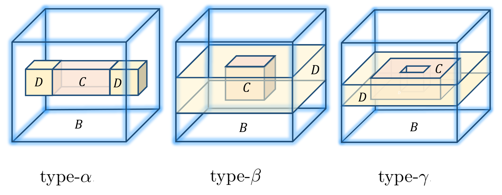
Type- has , which consists of two disconnected boxes, while is connected, and it can be used to detect open string-like , which is attached to the two boxes of . Type- has of the topology of a solid torus (and therefore is not simply connected), while is simply connected. It can be used to detect open membrane-like supported on which create excitations in as noncontractible loops. Type- has and of the same topology, e.g. the topology of a solid torus, and is simply connected.
Type- and type- have already been implied in paper by Kim and Brown [12], in which, similar subsystems types are used to study different types of boundaries of 3D models.
For type-, for models satisfying the assumptions in [13], e.g. the entanglement entropy of a general subsystem (which has large size compared to correlation length) can be decomposed into local plus topological parts:
Therefore, a model with is a model beyond the description of [13]. Fractal models do have for some choices of the subsystems and the value can be extensive. Furthermore, the contribution of () is not necessarily from open string-like (open membrane-like) .
III.2.2 The 3D Toric Code model has saturated lower bounds for each subsystem type
Let us go back to the 3D toric code model.
For type-, we find , where the operator is an open string operator which creates a point-like topological excitation in each box of and is a closed membrane operator. Therefore and .
For type-, we find , where the operator is an open membrane operator which creates a loop-like topological excitation at the edge of the membrane (the loop could not continuously shrink within into a point), and is a closed string operator. Therefore and .
For type-, operators supported on , which create excitations in , could always be deformed into . This is because, for 3D toric code, the operators that create topological excitations can be topologically deformed keeping the excitations fixed. Therefore we obtain a lower bound .
III.3 The X-Cube Model
The X-cube model is a 3D exactly solved stabilizer model, and it is an example of type I fracton phase [18]. The model is defined on a cubic lattice with one qubit on each link. The Hamiltonian is
| (12) |
where is a product of on a cube (which includes 12 links), and , , and are products of of 4 links around a vertex which are parallel to the -plane, -plane, -plane respectively.
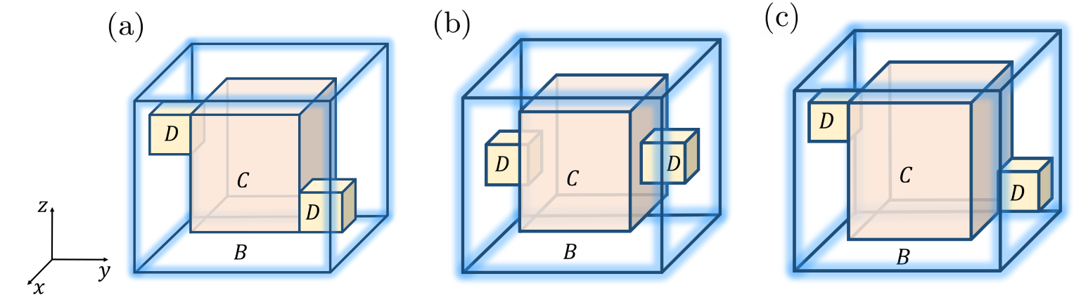
Here we focus on type- and consider the geometry dependence of , see Fig.7. We find the following lower bounds:
Fig.7a, ;
Fig.7b, ;
Fig.7c, .
Where denotes order one contributions which dependent on the detailed shapes of the subsystems, which is not crucial for our discussion.
The types of that contribute to the in Fig.7a are illustrated in Fig.8a, each stretches out in directions parallel to the -plane and creates a pair of “dimension-2 anyons.” The translations of the operators in Fig.8a in direction give you distinct operators (while translations in or directions do not give you distinct operators). This gives .
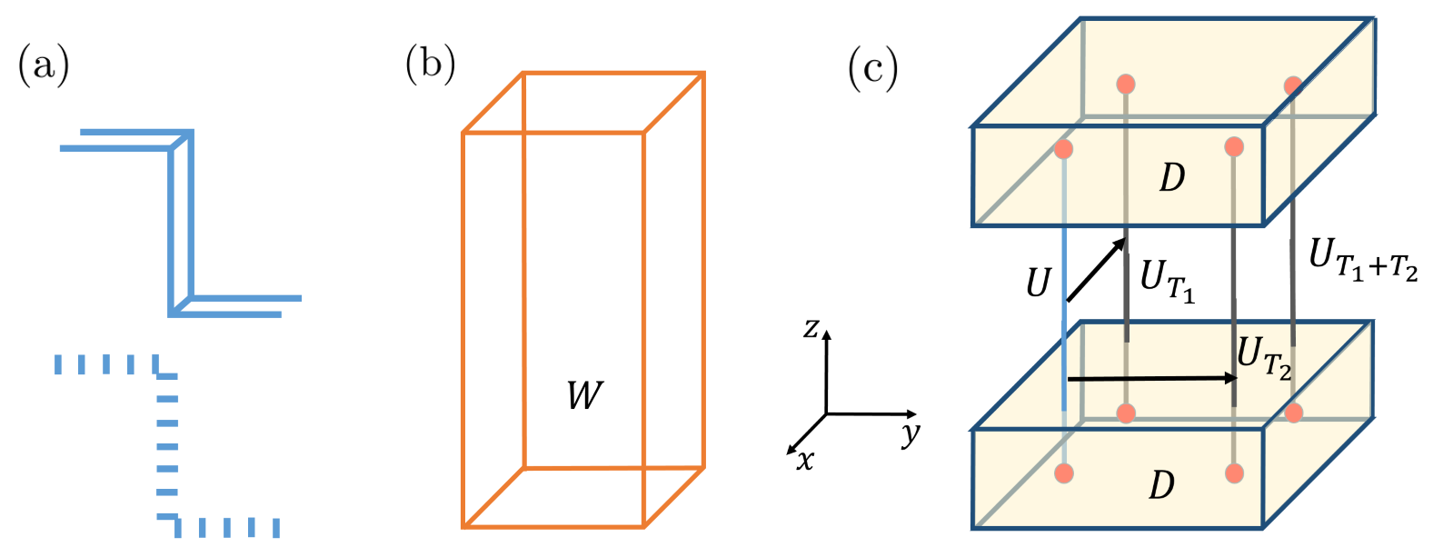
Translations can produce distinct operators, this indicates a breakdown of topological deformation: in the X-cube model, is deformable but not topologically deformable. Another nice example of the breakdown of topological deformation is shown in Fig.8c, in which and its translations , , and are distinct; nevertheless, by thinking of the condensate in Fig.8b, one can show .
The result for Fig.7b can be understood by thinking of contributions from operators parallel to the -plane and the -plane, which gives . The result in Fig.7c comes from the fact that the types of discussed above could not connect the two boxes of separated by a displacement vector with and the inability to find gives .
These results for may also be calculated using the method in [34] and an independent estimation agrees with our lower bounds up to contributions.
The lower bounds of for all the cases in Fig.7 depend on the length scale and the displacement vector but are not sensitive to other details. This is due to the fact that we have chosen “big enough” , so that they do not block any . If we consider another extreme, say the subsystem has a very narrow neck, then will be sensitive to the geometry of the neck which determines how many could pass through.
One may also apply the same idea to subsystems of type- and type- and find extensive values of and for certain choices of subsystems.
III.4 Fractal spin liquids
Fractal spin liquids [16] is a generalization of Haah’s code [15]. A common feature of fractal spin liquid models is the existence of fractal condensates. Fractal structures have discrete scale symmetries, and this results in a more complicated dependence of the ground state degeneracy on the system size [6, 16] compared to the type I fracton models.
Some of the fractal models possess “hybrid” condensates having both 1D parts and fractal parts, and the truncations of the condensates give you which can be either a string-like operator or a fractal operator. Note that, they do not fit into the definition of type I due to the existence of fractal operators. On the other hand, they do not fit into type II because the excitations created by the string-like operator are mobile excitations. Some fractal models have only fractal condensates, and no string-like exists. These models are type II fracton models.
Discussed in the following are ways to detect string-like and fractal using condensates. Then, is shown to be extensive for certain choices of subsystem geometry.
III.4.1 The Sierpinski Prism Model

As an example, we consider the model (d) in Yoshida’s paper [16]. Let us call this model the Sierpinski prism model, named after the shape of the condensate in Fig.9a, which looks like a prism with three legs decorated with Sierpinski triangles. This model lives on a 3D cubic lattice with two qubits ( and ) on each site. The Hamiltonian can be written as
| (13) |
where are integers labeling the sites on cubic lattice, and the Hamiltonian involves all the translations of the operator and . Explicitly, in terms of Pauli operators acting on each and qubit on different sites, we have
It is easy to check that all terms in the Hamiltonian commute and .
Using Yoshida’s notation:
Where , and . In terms of polynomials , with coefficients over , i.e. the coefficients can take 0 or 1:
Here and for the Sierpinski prism model. The polynomials with coefficients indicate the locations and the numbers of Pauli or operators in the product; the upper row is for qubits and the lower row is for qubits.
Choosing other polynomials , or changing into ( prime number) will generally give you other fractal models.
The Sierpinski prism model possesses hybrid condensates which consist of 1D parts and fractal parts, see Fig.9. The condensates in Fig.9a and Fig.9b can be constructed as a product of and the condensate in Fig.9c can be constructed as a product of . As is suggested by the discrete scaling symmetry of fractal structure and the continuous scaling symmetry of a 1D line: the upper and lower surfaces can be separated by an arbitrary distance in -direction (without changing the size of upper/lower surfaces), and under a rescaling the condensates look similar. Under other rescaling factors, the condensates look different but they could be constructed using a product of condensates that looks similar to the ones in Fig.9.
While this model does not have any logical qubits under periodic boundary conditions on an lattice, i.e. , it does have logical qubits under some “twisted” boundary conditions (say , , with , , and integer ), or under open boundary conditions.
Despite the fact that the Sierpinski prism model is one of the simplest fractal models, it nicely illustrates all the important ingredients needed in order to understand how our method works in fractal models. To be specific, it illustrates the following three types of detections:
1) The detection of a string-like using a fractal .
2) The detection of a fractal using a string-like .
3) The detection of a fractal using a fractal .
III.4.2 The detection of sting-like by fractal
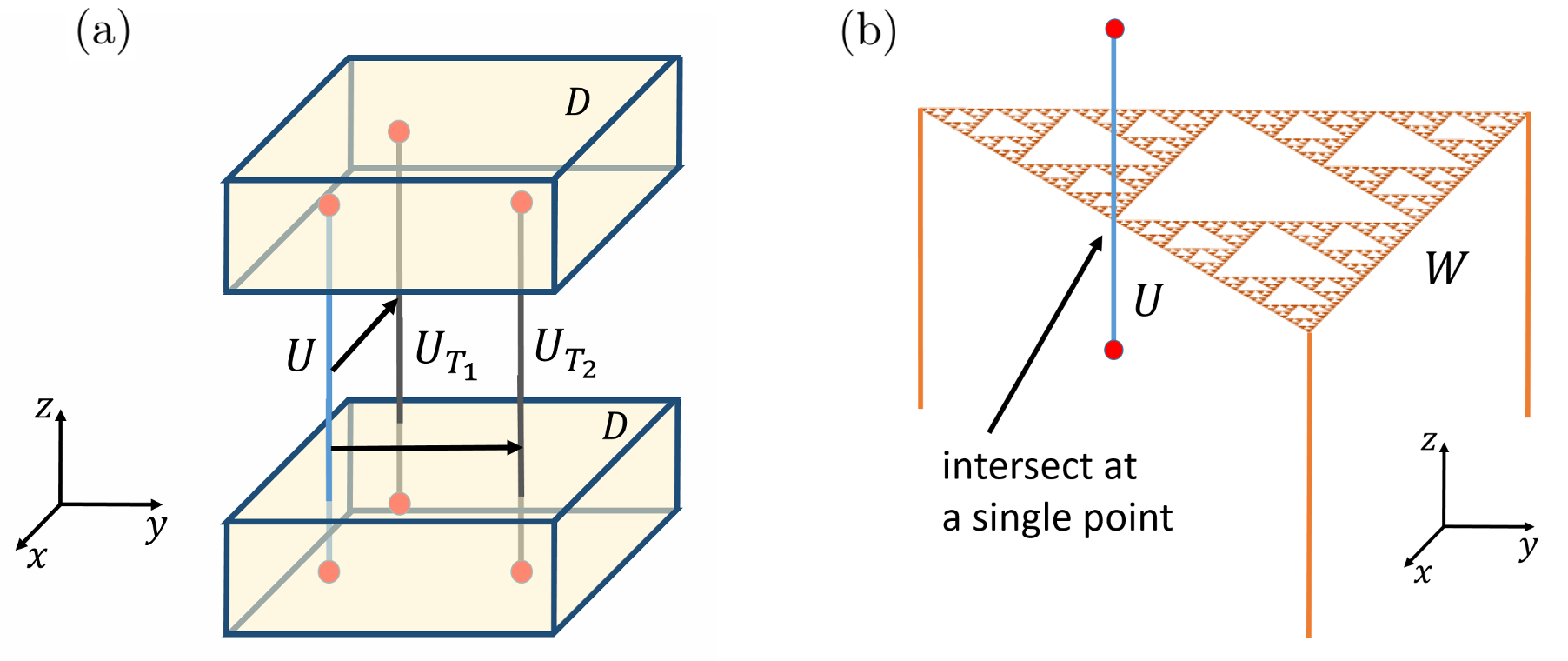
As is shown in Fig.9, we have condensates with string-like parts and fractal parts. String-like can be obtained from a truncation of the condensates. In Fig.10a, translations of a string-like , e.g. and (with , and an integer ) are distinct from , but . It is different from what happens in conventional topological orders but similar to what happens in type I fracton models, see Fig.8.
The distinctness of a string-like and its translations indicates a lower bound of extensive in the subsystem size, and indeed we can use the fractal part of to detect different string-like , see Fig.10b, and get an extensive lower bound.
III.4.3 The detection of fractal by string-like

Very similarly, fractal can be detected by string-like parts of , see Fig.11a. It is clear that a translation of a fractal will be a distinct operator if it anticommutes with a different . Therefore, by suitably choosing the geometrical shapes of subsystems , it is possible to get an extensive lower bound of . and .
III.4.4 The detection of fractal by fractal
Another way to detect fractal is to use a fractal part of a condensate , see Fig.11b, and it is the only way to detect for those fractal models without string operators i.e., when the condensates contain only a fractal structure without string-like parts (i.e., type II). Therefore, it is important to understand this case.
The key features, which can be observed in Fig.11b are the following.
1) The fractal condensates are supported on 2D surfaces with “holes” of different (discrete) length scales, in other words it is less than 2D.
2) Fractal and fractal (part of) lie in distinct intersecting surfaces, and it is possible to make the operators intersecting at a point. Certain translation of has a non-overlapping support with and therefore it commutes with . This implies that translations of can give you distinct operators.
After some thought, one finds it is possible to get an extensive lower bound of , and by suitably choosing the geometrical shapes of the subsystems . A choice of for type- or type- is shown in yellow color in Fig.11b.
III.4.5 Further comments
1) One may consider other subsystem types, for example: type- with consists of three disconnected boxes, and suitably chosen . When putting the three boxes on the positions of the three excitations of a in Fig.11, .
2) When rescaling the subsystem sizes according to the discrete scale symmetries (for the Sierpinski prism model, it is ), the change of could be investigated using entanglement renormalization group transformation [25]. For a rescaling by a factor which is not in the discrete scaling group, may change in more complicated way.
3) It is possible to have a fractal model with a unique ground state on a , in which case, there still exists nonzero . This indicates that is in some sense more universal than the ground state degeneracy.
4) For models with only fractal condensates (i.e. type II), although it is possible to find for some choices of , we get a lower bound when, for example, the two boxes of of length are separated by a displacement vector satisfying with some constant depending on the model. It might be a general exact result that when no matter how you choose but we do not have a proof. The case for Haah’s code is a conjecture by Kim 11 1 I. H. Kim, private communication. . If the conjectured results are true, this may be used to make a clear distinction between type I and type II fracton models.
IV Perturbations
The stability of quantities under local perturbations is an extremely important topic. If some property of an exactly solved model is totally changed when a tiny local perturbation is added, this property could never be observed in real systems.
The ground state degeneracy of topological orders is robust (stable) to arbitrary local perturbations. It is known that the toric code model is stable under arbitrary local perturbations [7]. The stability of ground state degeneracy is proved [2, 3] for a very general class of models which satisfy assumptions TQO-1 and TQO-2. In the proof, Osborne’s modification [35] of the quasi-adiabatic continuation [36] is employed. This proof is applicable to both conventional and fracton topological orders.
We would like to understand the stability of under local perturbations. It turns out that the stability of is a trickier problem compared to the stability of the ground state degeneracy. The corresponding problem for the conventional topological orders, e.g. the stability of topological entanglement entropy is not solved completely without additional assumptions. It is known from Bravyi’s counterexample (see [37] for a published reference) that the arguments provided in the original works [8, 9] about the invariance of the topological entanglement entropy under perturbation are not complete. Kim obtained a bound of the change of topological entanglement entropy with a st order perturbation [38] assuming the conditionally independence of certain subsystems.
Here we study the stability of our lower bound of under a finite depth quantum circuit for simplicity, since it is known from the viewpoint of quasi-adiabatic evolution [36] that local perturbations for gapped systems can be approximated by finite depth quantum circuit [39, 40].
Assumption : For subsystems , , as is shown in Fig.12. is a unitary operator which has support intersecting with and . is separated from by a distance . is a density matrix of a state with correlation length and replica correlation length [37] and . And is a density matrix such that
| (14) |
where “” means there is a correction that is negligible when is large compared to and .
The assumption should be understood as an assumption about the density matrix . It is trivial to check that “” can be replaced by “” when , and it may seem intuitive that the difference between the left-hand side and the right-hand side of Eq.(14) should decay as . Nevertheless, the original suggestion [8] that is true for is violated in Bravyi’s counterexample. It is observed in [37] that this is due to the fact that the replica correlation length is infinity for the cluster state in Bravyi’s counterexample. When the cluster state is deformed, becomes finite. For generic local perturbations without symmetry requirement, it is fine-tuned to have but can be arbitrarily large compared to . Judging from a recent conjecture [37] , may be the condition required for to be true.

In the following, we discuss the stability of our lower bound of under a depth- quantum circuit which creates a perturbed ground state satisfying . We take , and assume and much smaller than the length scales of the subsystems. This analysis does not cover all possible local perturbations (especially those with ), but we believe it covers a large class of interesting local perturbations.
Let be the depth- quantum circuit () which is responsible for the local perturbation. In other words, we assume the following objects in the perturbated model are related to the corresponding objects in the unperturbed model by
1) The new Hamiltonian: ;
2) The new (dressed) operators: , , and ;
3) The new ground state: ;
4) The new density matrices: and .

The dressed operators typically have a “fatter” support than the corresponding operators in the unperturbed stabilizer model, see Fig.(13) for an illustration. It is possible that the support of some will overlap with , the support of some will overlap with and the support of some will overlap with . For those operators, we need to throw them away, and supply with other operators if possible. We label the remaining operators using , , where , and we call the remaining density matrices , with , where .
With -1, -2, -3, -1, -2 satisfied for the unperturbed system, we supply with in order to complete a result about the stability of the lower bound. With these assumptions, one could verify the following results:
) -1, -3 and ;
) -1, -2 for ;
) -1, -2, -, .
The derivation of ) and ) are parallel to what is done in Sec.II.4. The derivation of ) follows. There exists a unitary operator supported on a region within a distance around , See Fig.14, such that , and . is some unitary operator supported on . It is always possible to find such and given that -2 is satisfied for the unperturbed case.
Therefore, .
Then, by applying -, -, and we find that
After simple algebra one arrives at the result ) i.e. .

Assuming the error caused by “” could be neglected, one could apply the same method as Sec.II.4 to arrive at a lower bound
| (15) |
For models with topologically deformable operators, like the 2D, 3D toric code models, our lower bound is invariant under perturbation. Because we can always move the excitations deep inside , such that the distance from any excitation to the boundary . For large subsystems, we would have and we do not lose any , and .
For models with not topologically deformable, e.g. the X-cube model and fractal spin liquids. There is usually some excitation that could not be moved deep inside subsystem . Therefore, after adding perturbations, we typically lose a few and , such that and . But for large subsystems which possess extensive before perturbation is added, this modification is small comparing to the leading contribution.
To summarize, for local perturbations satisfying assumption , and subsystem sizes much larger than and we expect:
| (16) |
For conventional topological orders , and for fracton topological orders being a number depends on the model and subsystem geometry.
V Discussion and Outlook
In this paper, we have obtained a lower bound of the nonlocal entanglement entropy from assumptions about the topological excitations and the ground state condensates of Abelian topological orders and applied our method to several examples. For conventional topological orders, e.g. the 2D toric code model and the 3D toric code model, our lower bounds are saturated and topologically invariant. Whenever the lower bound is saturated, we get an explicit construction of a conditionally independent density matrix . For fracton topological orders [14, 5, 15, 16, 17, 18], e.g. the X-cube model and the Sierpinski prism model, our lower bound depends on the geometry of the subsystems and is extensive for certain subsystem choices.
This method observes an intimate relation between and the topological excitations and the ground state condensates, and it obtains a lower bound of without calculating the entanglement entropy of any subsystem. A nonzero lower bound of is a result of the nonlocal nature of topological excitations, i.e. the fact that topological excitations could not be created alone by local operators. This nonlocal nature of topological excitations does not guarantee the operators which create the topological excitations to be topologically deformable and is not necessarily a topological invariance. Geometry-dependent is what appears in fracton models. It is beyond an established paradigm, i.e., the topological entanglement entropy, and should be treated as its generalization. The stability of the lower bound is discussed for local perturbations satisfying assumption , which should cover a large class of interesting local perturbations.
The different behaviors of may be used to distinguish fracton topological orders from conventional topological orders. Together with other methods being developed so far [11, 25], our result provides a better understanding of the entanglement properties of fractal models. Furthermore, the lower bound suggests (but not prove) different behaviors of between type I and type II fracton models. These different behaviors may be proven or disproven by later works.
Some of the assumptions in our method do not apply to non-Abelian models, a variant of our lower bound of for non-Abelian models is presented in [29]. Also, it might be interesting to investigate possible implications of our method on relations among topological order, topological entanglement entropy and quantum black holes [41, 42].
Acknowledgement
B.S. would like to thank Fuyan Lu for a comment on one assumption, Jeongwan Haah for providing a reference about Bravyi’s counterexample, Isaac H. Kim for a discussion and sharing one conjecture, and Michael Levin for a discussion about the entanglement in non-Abelian phases. This work is supported by the startup funds at OSU and the National Science Foundation under Grant No. NSF DMR-1653769 (BS,YML).
References
- [1] X. G. Wen and Q. Niu, Phys. Rev. B 41, 9377 (1990), URL http://link.aps.org/doi/10.1103/PhysRevB.41.9377.
- [2] S. Bravyi, M. B. Hastings, and S. Michalakis, Journal of mathematical physics 51, 093512 (2010).
- [3] S. Bravyi and M. B. Hastings, Communications in mathematical physics 307, 609 (2011).
- [4] M. A. Levin and X.-G. Wen, Phys. Rev. B 71, 045110 (2005), URL https://link.aps.org/doi/10.1103/PhysRevB.71.045110.
- [5] S. Bravyi, B. Leemhuis, and B. M. Terhal, Annals of Physics 326, 839 (2011).
- [6] J. Haah, Communications in Mathematical Physics 324, 351 (2013), ISSN 1432-0916, URL http://dx.doi.org/10.1007/s00220-013-1810-2.
- [7] A. Kitaev, Annals of Physics 303, 2 (2003), ISSN 0003-4916, URL http://www.sciencedirect.com/science/article/pii/S0003491602000180.
- [8] A. Kitaev and J. Preskill, Phys. Rev. Lett. 96, 110404 (2006), URL http://link.aps.org/doi/10.1103/PhysRevLett.96.110404.
- [9] M. Levin and X.-G. Wen, Phys. Rev. Lett. 96, 110405 (2006), URL http://link.aps.org/doi/10.1103/PhysRevLett.96.110405.
- [10] S. V. Isakov, M. B. Hastings, and R. G. Melko, Nature Physics 7, 772 (2011).
- [11] I. H. Kim, Phys. Rev. Lett. 111, 080503 (2013), URL http://link.aps.org/doi/10.1103/PhysRevLett.111.080503.
- [12] I. H. Kim and B. J. Brown, Phys. Rev. B 92, 115139 (2015), eprint 1410.7411.
- [13] T. Grover, A. M. Turner, and A. Vishwanath, Phys. Rev. B 84, 195120 (2011), URL http://link.aps.org/doi/10.1103/PhysRevB.84.195120.
- [14] C. Chamon, Phys. Rev. Lett. 94, 040402 (2005), URL http://link.aps.org/doi/10.1103/PhysRevLett.94.040402.
- [15] J. Haah, Phys. Rev. A 83, 042330 (2011), URL http://link.aps.org/doi/10.1103/PhysRevA.83.042330.
- [16] B. Yoshida, Phys. Rev. B 88, 125122 (2013), URL http://link.aps.org/doi/10.1103/PhysRevB.88.125122.
- [17] S. Vijay, J. Haah, and L. Fu, Phys. Rev. B 92, 235136 (2015), URL http://link.aps.org/doi/10.1103/PhysRevB.92.235136.
- [18] S. Vijay, J. Haah, and L. Fu, Phys. Rev. B 94, 235157 (2016), URL http://link.aps.org/doi/10.1103/PhysRevB.94.235157.
- [19] D. J. Williamson, Phys. Rev. B 94, 155128 (2016), eprint 1603.05182.
- [20] M. Pretko, Phys. Rev. B 95, 115139 (2017), URL https://link.aps.org/doi/10.1103/PhysRevB.95.115139.
- [21] S. Vijay, ArXiv e-prints (2017), eprint 1701.00762.
- [22] H. Ma, E. Lake, X. Chen, and M. Hermele, ArXiv e-prints (2017a), eprint 1701.00747.
- [23] T. H. Hsieh and G. B. Halász, ArXiv e-prints (2017), eprint 1703.02973.
- [24] K. Slagle and Y. B. Kim, ArXiv e-prints (2017), eprint 1704.03870.
- [25] J. Haah, Physical Review B 89, 075119 (2014).
- [26] E. Dennis, A. Kitaev, A. Landahl, and J. Preskill, Journal of Mathematical Physics 43, 4452 (2002), eprint quant-ph/0110143.
- [27] H. Ma, A. T. Schmitz, S. A. Parameswaran, M. Hermele, and R. M. Nandkishore, ArXiv e-prints (2017b), eprint 1710.01744.
- [28] H. He, Y. Zheng, B. A. Bernevig, and N. Regnault, ArXiv e-prints (2017), eprint 1710.04220.
- [29] B. Shi and Y.-M. Lu, ArXiv e-prints (2018), eprint 1801.01519.
- [30] B. Ibinson, N. Linden, and A. Winter, Communications in Mathematical Physics 277, 289 (2008), ISSN 1432-0916, URL http://dx.doi.org/10.1007/s00220-007-0362-8.
- [31] K. Kato, F. Furrer, and M. Murao, Phys. Rev. A 93, 022317 (2016), eprint 1505.01917.
- [32] H. Bombin and M. Martin-Delgado, Physical Review B 78, 115421 (2008).
- [33] A. Hamma, P. Zanardi, and X.-G. Wen, Physical Review B 72, 035307 (2005a).
- [34] A. Hamma, R. Ionicioiu, and P. Zanardi, Phys. Rev. A 71, 022315 (2005b), URL http://link.aps.org/doi/10.1103/PhysRevA.71.022315.
- [35] T. J. Osborne, Physical review a 75, 032321 (2007).
- [36] M. B. Hastings and X.-G. Wen, Physical review b 72, 045141 (2005).
- [37] L. Zou and J. Haah, Physical Review B 94, 075151 (2016).
- [38] I. H. Kim, Phys. Rev. B 86, 245116 (2012), URL http://link.aps.org/doi/10.1103/PhysRevB.86.245116.
- [39] X. Chen, Z.-C. Gu, and X.-G. Wen, Physical review b 82, 155138 (2010).
- [40] J. Haah, Communications in Mathematical Physics 342, 771 (2016).
- [41] L. McGough and H. Verlinde, Journal of High Energy Physics 2013, 208 (2013), ISSN 1029-8479, URL http://dx.doi.org/10.1007/JHEP11(2013)208.
- [42] A. Rasmussen and A. Jermyn, arXiv preprint arXiv:1703.04772 (2017).