The origin of radio pulsar polarisation

I assume that radiation observed at any pulse longitude results from coherent combination of linearly polarised natural mode waves. These are represented as two monochromatic sinusoids:

where $\Delta\phi$ is the phase delay between the modes. The Stokes parameters for such waves are calculated from:

(Rybicki & Lightman 1979). The polarisation fractions and angle are calculated in the usual way:

It is assumed that the observed polarisation results from an intrinsic signal (likely produced directly by the emission mechanism) which has propagated through some intervening magnetospheric plasma, possibly located at the polarisation limiting radius (PLR, e.g. Petrova & Lyubarskii 2000). The intervening matter is represented by a polarisation basis $(\vec{x},\vec{y})$ and the signal enters the basis at a polarisation angle $\psi_{in}$ given by:

where $R$ is the mode amplitude ratio,

and $E$ is the incident wave amplitude. The PA observed in single pulses typically exhibits wide distributions at a fixed longitude, which are assumed to be caused by the stochastic nature of the input signal. I assume that typically a wide distribution of $\psi_{in}$, denoted $N_{\psi,in}$, which at some longitudes may possibly be even quasi-isotropic, enters the polarisation basis (different $\psi_{in}$ contribute at a given pulse longitude in different single pulses). The PA at which $N_{\psi,in}$ is maximum is denoted by $\psi_{pk}$, and the width of $N_{\psi,in}$ by $W_{\psi,in}$ .

The incident signal is split into components $E_{x}$ and $E_{y}$ parallel to the polarisation direction of the proper propagation modes in the intervening matter, which induces some phase lag $\Delta\phi$ between $E_{x}$ and $E_{y}$. The intervening matter is assumed to be highly modulated and irregular, hence the lag is also expected to be highly random, and represented by a wide distribution $N_{\Delta\phi}$ with the maximum at $\Delta\phi_{pk}$ and the width $W_{\Delta\phi}$. The whole propagation physics is parametrised with these two quantities.

It is assumed that the observed variations of polarisation as a function of pulse longitude²² 2 The capital letter $\Phi$ refers to the pulse longitude in the profile, and should not be mistaken with the small $\phi$ which denotes oscillation phase in the wave given by eq. (1). Hereafter I always use the word ‘longitude’ to refer to $\Phi$, whereas ‘phase’ is used for $\phi$. $\Phi$, mostly result from the longitude dependence of the mode ratio and phase lag, i.e.:

The function $\psi_{pk}(\Phi)$ is determined by the relative orientation of a distribution of incident PAs and the intervening basis, as described in Section 4.5. Since the emission and propagation physics is neglected, the other functions need to be found by a guess, hopefully guided by the qualitative properties of available data. Equations (11)-(14) make the Stokes parameters dependent on the pulse longitude.

Hereafter I will be interested in polarisation fractions and angle, since they depend only on the ratio $R=E_{2}/E_{1}$. This makes it possible to ignore the absolute profiles of $I$, $L$ and $V$, i.e. the incident wave amplitude $E=1$ in eqs. (10).³³ 3 Unfortunately, in observational works usually only the observed $I$, $L$ and $V$ are published. This makes it very difficult to assess $L/I$ and $V/I$ whenever $I$ is changing steeply or is very low. This plotting tradition seriously hampers any attempts to interpret the observed pulsar polarisation.

The polarisation angle $\psi$, as given by eq. (8), so far only includes the effects of mode addition, without the likely variations caused by the changes of projected magnetic field with $\Phi$. If these regular RVM variations of PA are denoted as $\psi_{\scriptscriptstyle RVM}(\Phi)$, the observed PA is:

i.e. $\psi_{\scriptscriptstyle RVM}$ serves as a reference value for the non-RVM effects.

It is then assumed that the input wave becomes split into components parallel to the natural polarisation directions, then the components acquire some phase lag $\Delta\phi$, and finally combine. Fig. 2 presents the polarisation characteristics for $\Delta\phi$ values within one full wave oscillation period, and for a set of mode amplitude ratios that correspond to the input PA values separated by $5^{\circ}$. The bottom panel presents the PA as a function of the phase lag, with $\psi_{in}$ fixed on each curve of $\psi(\Delta\phi)$. For each point in the bottom panel, $\psi_{in}$ can be established by following the closest curve of $\psi(\Delta\phi)$ towards the left vertical axis, i.e. $\psi_{in}=\psi(\Delta\phi=0)$. The PA of the natural modes of the intervening polarisation basis is shown with the dot-dashed horizontal lines at $\psi=\pm 90^{\circ}$ and $0^{\circ}$ (the latter is overlapping with $\psi(\psi_{in}=0)$). The straight lines that correspond to equal mode amplitudes (incident PA of $\pm 45^{\circ}$, hereafter called intermodes) consist of separate sections that jump discontinously to orthogonal values at $\Delta\phi=90^{\circ}$ and $270^{\circ}$ (as marked with ticks and thick line sections). This corresponds to the transformation of the polarisation ellipse into a circle, and further into an orthogonally oriented ellipse (as shown near the top of the figure). Changes of $L/I$ and $V/I$ for this equal amplitude case ($\psi_{in}=45^{\circ}$) are shown in the top panel with thick lines, which clearly demonstrate the anticorrelation of $L/I$ and $|V|/I$ inherent for the CMA.

The orthogonal polarisation modes of radio pulsar emission clearly stand out at the locations where several different curves of $\psi(\Delta\phi)$ cross at the same point. In single pulse observations, at a fixed pulse longitude, different points of this figure are quasi randomly sampled, with some spread in the input PA ($N_{\psi,in}$, shown left of the plotting box) and some spread in the phase lag ($N_{\Delta\phi}$, shown below the plot).

The origin of these OMPs, emerging as the nodes in the lag-amplitude ratio diagram, is simple: the input signal which is polarised at an arbitrary $\psi_{in}$, produces polarisation ellipses parallel to either natural polarisation mode, whenever the lag $\Delta\phi=\pi/2$. That mode will be observed, which corresponds to the larger component of the split input vector.

The phenomenon is presented in Fig. 3a, in which components of a dotted electric field vector, tilted at an arbitrary input angle of $\psi_{in}=25^{\circ}$ combine at $\Delta\phi=90^{\circ}$ into the dotted polarisation ellipse, whereas another input vector at $\psi_{in}=65^{\circ}$ (solid), similarly produces the solid ellipse. This way the two orthogonal modes, always polarised at $0^{\circ}$ or $90^{\circ}$ are produced.⁴⁴ 4 The PA, $L$, and $V$ of the elliptically polarised radiation are determined assuming decomposition into the fully circular part, and the phase coherent linear part in the direction of the major axis of the ellipse. If $\Delta\phi$ is slightly different from $90^{\circ}$, the polarisation ellipses are no longer strictly parallel to the $\vec{x}$ or $\vec{y}$ vector of the basis, however, for most $R$ the misalignment is small (this can be seen by making a vertical cut through Fig. 2, e.g. at $\Delta\phi=80^{\circ}$). If the input vectors appear on both sides of the dashed diagonal in Fig. 3a, the two orthogonal modes will be present in the observed signal whenever the medium imposes phase delays in the vicinity of $\pi/2$ on the propagating signal. If $\Delta\phi\neq\pi/2$, variety of PA values will be observed, however, their fixed-longitude distributions will reveal maxima at the modes. This can be understood by considering the local line density along some vertical cut of Fig. 2 (any vertical slice which is not at a multiple of $\Delta\phi=\pi$). Thus, the modes will emerge statistically in the observations, even for phase lags much different from $90^{\circ}$, although in such case they will form a distribution with wide peaks connected with bridges. Therefore, if the lag and $\psi_{in}$ are sampled from a wide or random distribution, the modes stand out clearly in statistical sense, i.e. appear frequently.

When both the distributions ($N_{\psi,in}$ and $N_{\Delta\phi}$) are uniform, the bottom panel of Fig. 2 will not be uniformly covered by samples. Instead, the PA observed in different samples will bunch at the orthogonal modes, following the density of the lines in the figure. In spite of the pure randomness of input polarisation parameters, the orthogonal modes will anyway stand out in single pulse observations with equal strength, but the average profile will be fully depolarised. The apparent OPMs generated through the coherent mode combination are then an extremely robust feature, easily surviving most of sampling styles that can be imagined for Fig. 2. Only the zero lag, or a multiple of $\pi$, does not produce the OPMs.

In other words, the density of lines in Fig. 2 presents the probability of measuring a given PA for a totally random orientation of the input polarisation and for a random (uniform) distribution of phase lags (by ‘measuring’ I mean the measuring of PA at short time samples always taken at a fixed pulse longitude). Equations (8), (3), and (4) give

A square equation $R^{2}+2KR-1=0$ gives the solution for $\psi_{in}(K)$, which provides the input PA for any point in Fig. 2: $\psi_{in}(\Delta\phi,\psi)$. The above-described probability distribution (for the uniform $N_{\psi,in}$ and $N_{\Delta\phi}$) is then calculated as the rate at which the lines of fixed $\psi_{in}$ are crossed vertically:

and is presented in Fig. 4.

If $N_{\Delta\phi}$ in Fig. 2 is narrow, whereas $N_{\psi,in}$ is very wide (or isotropic) then clearly defined OPMs will be observed when $N_{\Delta\phi}$ peaks near $\Delta\phi=90^{\circ}$ or $270^{\circ}$. If the peak of $N_{\Delta\phi}$ is at $\Delta\phi=0^{\circ}$, $180^{\circ}$, or a multiple of thereof, the quasi-uniform distribution of the input PA will be observed. Intermediate cases produce wide observed PA distributions, with broad tracks of quasi-orthogonal modes, and many PA values between them. Inclusion of a narrow PA distribution (shown on the left in Fig. 2) further modifies the picture, as will be described below.

For a symmetrical orientation of input vectors with respect to $\psi_{in}=45^{\circ}$, equal amounts of same-handedness circularly polarised signal are produced (Fig. 3a). It is important to note that this case is different from the case when the input signal is split into two natural orthogonal modes which are elliptically polarised and reach the observer without being combined on the way. In the last case the handedness of $V$ is opposite (Fig. 3c) and the resulting $V=0$. A symmetrical distribution of the input PA, centered at $\psi_{in}=45^{\circ}$ (marked with the dashed line in Fig. 3a) will produce equal amounts of the two OMPs plus strong $V$. The same distribution centered at $\psi_{in}=90^{\circ}$ (or $0^{\circ}$) will produce one strong polarisation mode with little $V$, as illustrated in Fig. 3b. This is again different from the elliptical mode case, in which a single mode signal should reveal the elliptical polarisation intrinsic to the natural propagation mode.

It is a notable feature that for the vectors located on different sides of $\psi_{in}=45^{\circ}$ (Fig. 3a) the orthogonal OPMs are produced with the same handedness of circular polarisation. This phenomenon is observed in the single pulse emission, where samples of the same handedness appear on both orthogonal mode PA tracks. This is well illustrated in Figs. 1 and 2 of Mitra et al. (2015) who plot opposite-handedness samples in different colors.

Another very important point is that in the case of the coherent mode addition $V$ changes sign when the peak of the input PA distribution moves across one of the natural modes (Fig. 3b). Therefore, different samples of the same polarisation mode may have opposite sign of $V$, as can also be seen in Figs. 1 and 2 of MAR15.

Both the above-described properties are opposite to what is known about the noninteracting elliptically polarised propagation modes.

As shown in Fig. 3a the answer to the question of which mode will be detected, depends on the orientation of the input polarisation vector with respect to the separating angle of $45^{\circ}$. Accordingly, in the case of symmetrical $N_{\psi,in}$ distributions that peak at $\psi_{pk}$, the predomination of a given mode depends on the position of $\psi_{pk}$ relative to $45^{\circ}$.

To learn what Stokes parameters contribute at a given pulse longitude, $N_{\psi,in}$ and $N_{\Delta\phi}$, shown on the margins of Fig. 2, must be convolved with the line density distribution on the lag-PA diagram. The convolution of $N_{\Delta\phi}$ is simple: the lag distribution selects the whole vertical area in Fig. 2, located directly above $N_{\Delta\phi}$, and the contribution of different phase lags to the average signal is weighted by $N_{\Delta\phi}$. The PA distribution on the left, however, is convolved indirectly: for the input PA of, say, $40^{\circ}$, it is necessary to start at this value on the left axis of Fig. 2, and follow the fixed $\psi_{in}$ line rightwards, until the vertical region selected by the lag distribution is reached. This implies that whenever the PA distribution extends to both sides of $\psi_{in}=45^{\circ}$, both OPMs are produced and they may appear in single pulse data (at a given phase in different rotation periods, i.e. they may be visible as the parallel tracks of orthogonal PA).⁵⁵ 5 The visibility of both OPMs is known to depend on the question of whether the two OPMs, i.e. the different results of the coherent addition, can simultaneously contribute to a single time sample (Stinebring et al. 1984; McKinnon & Stinebring 2000). For $N_{\psi,in}$ which does not extend beyond the interval of $[-45^{\circ},45^{\circ}]$ (or beyond $[135^{\circ},215^{\circ}]$), a single OPM will be observed.

An arbitrary example of combined effects of $N_{\psi,in}$ and $N_{\Delta\phi}$ is shown in Fig. 5, where a moderately wide PA distribution peaking at $\psi_{in}=30^{\circ}$, and a lag distribution peaking at $\Delta\phi=60^{\circ}$, generate two approximately orthogonal polarisation modes of unequal magnitude (at $\Delta\phi\approx 90^{\circ}$). The thickness of $\psi(\Delta\phi)$ curves in that figure is made proportional to the product of appropriate values in the distributions: $N_{\psi,in}(\psi_{in})N_{\Delta\phi}(\Delta\phi)$, where $\psi_{in}$ should be understood as $\psi_{in}=f(\psi,\Delta\phi)$. The imperfect orthogonality of OPMs, often observed in pulsars, is a natural consequence of the convolution presented in Fig. 5.

The PA and lag distributions do not necessarily need to be as narrow as shown in Fig. 2. In particular, $N_{\Delta\phi}$ can span much more than $2\pi$. The resulting polarisation characteristics are then a residual effect determined by the horizontal misalignment of $N_{\Delta\phi}$ with respect to vertical symmetry lines of the lag-PA pattern (e.g. $\Delta\phi=90^{\circ}$, or $180^{\circ}$). Possible asymmetry of the lag distribution wings could also be in such case decisive for the ensuing PA.

The PA curve of B1913$+$16 (Weisberg and Taylor 2002, reproduced here in Fig. 1), if considered alone, looks quite innocuous: there are three PA flattenings that seem to present the two natural OPMs separated by two gradual transitions between them. However, $|V|/I$ astonishingly peaks at the transitions (instead of crossing zero), and both the transitions are gradual. Equally strange, $L/I$ is high everywhere (top grey line in Fig. 1). Instead of reaching zero, $L/I$ decreases near the trailing PA jump from $0.65$ to $0.45$.

Since generally $|V|/I>0$ in the profile, the peak $\Delta\phi_{pk}$ of the $N_{\Delta\phi}$ distribution must either be displaced from zero, or the distribution must be asymmetric, because otherwise $V$ would vanish (e.g. see Fig. 3b, and note that a change of the lag from $\pi/2$ to $-\pi/2$ is equivalent to a change of sign in one component of the incident vector). Two examples of such distributions (denoted $N_{\Delta\phi}$) are shown on the left margin of Fig. 6. The asymmetric $N_{\Delta\phi}$ with only positive $\Delta\phi$ is expected for the PLR scenario (Cheng & Ruderman 1979; Lyubarskii & Petrova 1998; ES04) although both the distributions often produce similar results if the symmetric one is not too wide and is displaced to some $\Delta\phi_{pk}>0$.⁶⁶ 6 The observation of slightly elliptical modes by ES04 in B0329$+$54 is not necessarily inconsistent with the PLR effects on the purely linear natural modes, because the observed OPMs are the net result of the coherent combination of the natural propagation modes with some $N_{\psi,in}$ and $N_{\Delta\phi}$. A slight asymmetry of $N_{\psi,in}$ (and $N_{\Delta\phi}$) around zero is sufficient for the observed mode to acquire some ellipticity even when the natural modes are perfectly linear (Fig. 3b). Still, the natural elliptical modes are supported by the observed OPM jumps at which $V$ does change the sign. For simplicity I ignore this ellipticity in this paper.

If the small positive $V/I$ on the leading edge of the profile is ignored ($\Phi\approx-20^{\circ}$ in Fig. 1), a sinusoid-like $V/I$ is observed in the rest of the pulse window, i.e. $V/I$ decreases from zero to a negative minimum at $\Phi=-7^{\circ}$, crosses zero at $7^{\circ}$, reaches maximum at $\Phi=15^{\circ}$ and finally drops to zero at the trailing edge. Since $V$ should change sign whenever $\psi_{pk}$ coincides with one of the natural modes, the observed $V$ profile suggests that the input vector must rotate by slightly more than $180^{\circ}$, say between the values of $-100^{\circ}$ and $100^{\circ}$ in Fig. 6. This interval of $\psi_{in}$ is hereafter assumed to be cast onto the observed pulse window of B1913$+$16. The initial position of the $N_{\psi,in}$ distribution is shown at the bottom of the figure, and it is assumed to roughly correspond to the leading edge of the observed profile. While the pulsar rotates, $N_{\psi,in}$ moves rightwards.

The top panel of Fig. 6 shows the probability distribution that needs to be convolved with $N_{\psi,in}$ and $N_{\Delta\phi}$ to determine the polarisation characteristics at a given longitude. In a general case of arbitrary distributions, the procedure is as follows: for each pulse longitude (i.e. for a given position of $N_{\psi,in}$ at $\psi_{pk}$) the Stokes parameters, as determined by $\Delta\phi$ and $\psi_{in}(\Delta\phi,\psi)$, need to be integrated over $N_{\Delta\phi}$ to obtain the observed distribution of PA (i.e. $\psi$) at a fixed $\Phi$ (or distributions of $L/I$ and $V/I$ at that $\Phi$). To obtain a single value of PA in an average profile, the integration needs to be done over both $N_{\Delta\phi}$ and $N_{\psi,in}$.

For B1913$+$16 I employ moderately narrow distributions, which makes it possible to read out the result directly from Fig. 6. The modal peaks, located at $\psi_{in}=0$ and $\pm 90^{\circ}$ in the $P$ distribution (top panel) are very strong features. Therefore, when $N_{\psi,in}$ (i.e. $\psi_{pk}$) coincides with one of the modal PA values at some pulse longitude $\Phi$, that OPM value statistically dominates in single pulse samples observed at that $\Phi$. In other words, the peak of the convolved net probability distribution will be located close to the modal peaks. However, if $N_{\psi,in}$ is located at an intermode (e.g. $\psi_{pk}=45^{\circ}$), then the modal points are located in the low-level wings of both $N_{\psi,in}$ and $N_{\Delta\phi}$. The strongest (most likely) contribution then comes from the location in the $(\psi,\Delta\phi)$ diagram which corresponds to the peaks of $N_{\psi,in}$ and $N_{\Delta\phi}$. For the symmetric $N_{\Delta\phi}$ distribution shown on the left margin of Fig. 6, this corresponds roughly to $(\psi,\Delta\phi)=(45^{\circ},40^{\circ})$.

Therefore, the steady motion of $N_{\psi,in}$ along the horizontal axis of the diagram (as caused by the pulsar rotation) translates into the wavy thick arrow marked in the bottom part of all panels in Fig. 6. The observed polarisation will be dominated by the Stokes parameters recorded along this thick wavy line. Accordingly, Fig. 6 provides $L/I$ (middle panel) and $V/I$ (bottom panel) with the same wavy track as in the top panel.

In agreement with the observed properties of B1913$+$16, at both OPM transitions ($\psi_{in}=\pm 45^{\circ}$) the wavy line omits the region of low $L/I$ (bright in the middle panel), staying much larger than zero for all the time. $|V|/I$ is maximum at the OPM transitions ($\psi_{in}=\pm 45^{\circ}$), and $V$ changes sign in the middle ($\psi_{in}=0$), in the region dominated by one polarisation mode.

A numerical code which convolves Gaussian distributions of $N_{\psi,in}$ and $N_{\Delta\phi}$ gives the result shown in Fig. 7.⁷⁷ 7 For each longitude $\Phi$, i.e. for a given $\psi_{pk}$ and $\Delta\phi_{pk}$, the code simply runs over the $\psi_{in}$ and $\Delta\phi$ loops and calculates the Stokes parameters scaled by $N_{\psi,in}N_{\Delta\phi}$. A calculation of $\psi$ then makes it possible to gather the Stokes in separate arrays indexed by $\psi$ and $\Phi$. It is obtained for $\Delta\phi_{pk}=40^{\circ}$, $\sigma_{\Delta\phi}=70^{\circ}$ and $\sigma_{\psi,in}=30^{\circ}$ (parameters selected to obtain a rough by eye fit). The value of $\psi_{pk}$ changes linearly as defined by the horizontal axis. This is likely unrealistic, but appears sufficient to reproduce the observed polarisation approximately (the full length of the $\psi_{pk}$ axis must be cast onto the pulse window of B1913$+$16). Modelled single pulse PA distributions (grey patches in Fig. 7) have the familiar form of OPM bands observed in other pulsars. In the intermode region (near $\psi_{pk}=\pm 45^{\circ}$) these bands overlap in $\Phi$, because one wing of $N_{\psi,in}$ distribution extends across the intermode value. Similar result is obtained for the $N_{\Delta\phi}$ distribution shown with the thin line on the left margin of Fig. 6. This is because in both cases one wing of $N_{\Delta\phi}$ reaches the modal points at $\Delta\phi=90^{\circ}$, and $\Delta\phi_{pk}$ is close to zero. Even if this last distribution is made symmetric around $\Delta\phi=0^{\circ}$, the PA would not change much, but $V$ would vanish.

The direction of the step-wise PA variations in B1913$+$16 (Fig. 7) is determined by the steady motion of $N_{\psi,in}$ towards larger $\psi_{in}$ with the increasing $\Phi$. The direction of OPM transition is not accidental in the model: within the modal transition the derivative $d\psi/d\Phi$ has the same sign as $d\psi_{pk}/d\Phi$. This tells us that $\psi_{pk}$ increases monotonically within the full pulse window of B1913$+$16, as marked in Fig. 6.

Although no RVM effect is included in the model, the PA curve is fairly similar to the observed one. The RVM PA (which may be considered constant at this stage of calculation) can be imagined as a perfectly horizontal line at $\psi=0$. It can be seen that neither the average PA nor the grey single-pulse PA track follow the horizontal line. This slope is introduced by the steady motion of $N_{\psi,in}$ across the natural mode at $\psi=0$. Therefore, in B1913$+$16 the slope of RVM PA is likely biased by the mode coherency effects, and is unlikely to be determined through the RVM fitting, unless a precise model of the coherent mode combination is included as a part of the RVM fitting procedure. Unlike in Fig. 7, the full span of the observed PA ($195^{\circ}$, as noted by Weisberg & Taylor 2002) exceeds $180^{\circ}$, which is the maximum possible value for the equatorward viewing geometry. This slight vertical extension is likely caused by the RVM, which only partially contributes to the PA slope observed in the middle of the profile.

If the $N_{\Delta\phi}$ distribution is very wide ($W_{\Delta\phi}\ga\pi$) or centered close to the modal points ($\Delta\phi\approx 90^{\circ}$) then thin well-defined bands of both OMPs extend for most of the profile at a longitude-dependent strength ratio (see Fig. 8). This is because the modal points on the $P(\psi,\Delta\phi)$ plane are always within the reach of $N_{\Delta\phi}$ and keep to be selected by $N_{\Delta\phi}$ for any $\psi_{pk}$. In Fig. 8 $V/I$ is close to zero because $\Delta\phi_{pk}=40^{\circ}$ is much smaller than $\sigma_{\Delta\phi}=130^{\circ}$ (symmetry of $N_{\Delta\phi}$ with respect to $\Delta\phi=0$ suppresses $V$). $L/I$ has the profile of $|\cos{2\psi_{pk}}|$ with deep minima at sharp OPM jumps.⁸⁸ 8 $L/I$ has the profile of $|\cos{2\psi_{pk}}|$, because the input signal of amplitude $E$, linearly polarised at an angle $\psi_{pk}$ with respect to one of the natural modes, produces two waves of amplitudes $E_{x}=E\cos\psi_{pk}$, and $E_{y}=E\sin\psi_{pk}$. If $N_{\Delta\phi}$ is very wide, i.e. the waves combine incoherently, then $L/I=|E_{x}^{2}-E_{y}^{2}|/(E_{x}^{2}+E_{y}^{2})=|\cos(2\psi_{pk})|$, i.e. $L/I$ vanishes four times per a single revolution of $\psi_{pk}$ (each time when the projected components are equal). As soon as $\sigma_{\psi,in}$ is increased above $\sim\negthinspace 50^{\circ}$, both sharp modes of similar amplitude are present at all $\Phi$ and there is a nearly complete depolarisation ($L/I=V/I\approx 0$). Overall, very wide distributions tend to depolarise for obvious reasons, however, the wide $N_{\psi,in}$ suppresses both $L$ and $V$ (at whatever width of $N_{\Delta\phi}$), whereas the wide $N_{\Delta\phi}$ suppresses $V$, but $L$ only at the modal transitions.

Moderately wide $N_{\psi,in}$ can produce broad clouds of PA centered at the modal values, with the average PA slowly traversing from one mode to another. The transition may occur at a small, but non-vanishing $L/I$ and $V/I$. Effects of this type are often observed (e.g. B0823$+$26 in Fig. 12 of MAR15, B2110$+$27 in Fig. 19 therein) and occur when $N_{\psi,in}$ is crossing the intermode and the widths of the distributions are moderate ($\sigma_{\psi,in}\sim 45^{\circ}$, $\Delta\phi_{pk}\sim 45^{\circ}$, $\sigma_{\Delta\phi}\sim 45^{\circ}$). Otherwise, i.e. for a large $W_{\Delta\phi}$, $N_{\Delta\phi}$ can reach the modal points on the lag-PA plane, and the observed modal tracks become narrow.

Two prototypical single pulse PA scatter plots are schematically presented in Fig. 9. The top one, based on B1237$+$25 (Fig. 1 in SRM13), shows the PA of an M-type profile (with multiple components, Rankin 1983; Backer 1976) and with a complicated PA distortion at the profile center. Similar distortions, associated with the core component, are also observed in B1933$+$16 and B1857$-$26. Double ‘conal’ profiles (Fig. 9b), on the other hand, exhibit the well defined S-shaped PA swing following a single OPM across the full profile, with roughly symmetric patches (short fragments of a PA track) of the secondary OPM in the profile peripheries. As shown in Fig. 9a, similar orthogonal PA patches also appear in the pulsars with the complex core properties (e.g. B1237$+$25). Unfortunately, in these objects the complexity of the central PA distortion often makes it difficult to consistently identify a single OPM throughout the whole pulse window. In B1933$+$16 the loop-like PA distortion converges back at the original (strong) mode. In B1237$+$25, however, the core PA loop spreads from the primary mode, but appears to converge at another, secondary mode, as identified by the short PA patch marked in Fig. 9a. Moreover, Mitra & Rankin (2008) note that flat sections of the PA curve observed in B1857$-$26 imply equatorward viewing geometry for which the full span of the RVM PA cannot exceed $\pi$, contrary to what seems to be observed, if the RVM is consistently attributed to the primary (strong) mode. The authors were then tempted to present a PA fit based on ‘unsavory assumption’ that the primary (brighter) mode on the leading side continues into the ‘patch mode’ on the right.

In principle, however, such change of mode identity (with the RVM continuing from the primary into the secondary mode) occurs naturally in the CMA model, whenever $N_{\psi,in}$ moves across $45^{\circ}$ and starts to mostly contribute to the other polarisation mode. This is because for a phase lag increasing from zero, the lines of fixed-$\psi_{in}$ in the lag-PA diagram (Fig. 10) diverge upwards for $\psi_{in}\ga 45^{\circ}$, whereas they diverge downwards for $\psi_{in}\la 45^{\circ}$. Thus, at an intermode the strength of the modes is exchanged and the primary mode becomes the patch mode. Such inversion of the mode amplitude ratio is also explained in Fig. 3a. This possibility allows one to construct a naive polarisation model of pulsars such as B1237$+$25 and B1857$-$26, which resembles the generic case shown Fig. 9a.

The core PA distortions look like fast modal transitions which have got reversed, or failed to be completed. As can be seen in Fig. 2, any manipulations with $N_{\Delta\phi}$ (displacements of $\Delta\phi_{pk}$ along the $\Delta\phi$ axis) do not allow us to leave the single mode space between the consecutive intermodes. On the other hand, a single passage of $\psi_{pk}$ through one of the intermodes (at $\pm 45^{\circ}$ or $\pm 135^{\circ}$) produces both the orthogonal transition of PA and a change of the modal amplitude ratio, thus redefining which mode is primary and which is secondary.

Still, such replacement of the mode illumination requires an odd number of intermode crossings, whereas the core PA loops have the ‘up-and-down’ form, which suggests an even number (on the way to another mode and back). Even in B1237$+$25 the odd-numbered transition of the core PA (from the primary to the secondary mode) is followed by one more PA transition back to the primary mode, at a trailing-side longitude where the core emission seems to cease and subdue to the peripheric emission.

In B1933$+$16 the core loop opens and closes at the same (say primary) mode, so it will now be interpreted in terms of the reversed mode transition with no mode identity replacement, as caused by nonmonotonic variations of $\psi_{pk}$. On the left side of the PA loop in B1933$+$16 (see Fig. 1 in MRA16) one polarisation mode dominates which means that $\psi_{pk}\sim 0$ and the observed $\psi$, $V/I$, and $L/I$ can be represented by the values at the median line of Fig. 7 (assuming similar $N_{\Delta\phi}$ distribution for B1933$+$16 and B1913$+$16). Let us assume that within the loop of B1933$+$16 $\psi_{pk}$ changes with $\Phi$ nonmonotonically, in the way which is presented by the backward-bent arrow in Fig. 7b. This qualitatively reproduces the major observed properties of the loop: while moving leftward $L/I$ decreases, $|V|/I$ increases, and the average PA almost makes the full OPM transition. Shortly after passing through the minimum in $L/I$ (at $\psi_{pk}=-45^{\circ}$), $\psi_{pk}$ starts to increase, immediately passing again through the $L/I$ minimum, and $|V|$ starts to drop.

Numerical simulation of such case is shown in Fig. 11, where simple linear changes of $\psi_{pk}$ were asumed ($\psi_{pk}$ in radians is shown in the bottom panel with a dashed line). Despite such linear variations of $\psi_{pk}$ are far from those expected at an even-numbered intermode crossing in pulsar magnetosphere (see Section 4.5) they produce polarisation similar to that observed. In particular, the modelled minima in $L/I$ have the characteristic twin-like look as in the data: they are close to each other, and connected with only a slightly increased $L/I$ in between them. The sharp tip at the center of $L/I$ and the slanted PA on both sides of the V-shaped PA feature (Fig. 11) are artifacts of the linear $\psi_{pk}$.

The V-shaped distortion of Fig. 11 does not extend beyond $\Delta\psi=90^{\circ}$ hence it does not have the loop-shaped form. The observed shape may be caused by a more complicated structure of $N_{\psi,in}$ than the Gaussian form assumed above. However, the observed loop can also be interpreted purely in terms of $N_{\Delta\phi}$ displacement, with a fixed $\psi_{pk}\sim 45^{\circ}$ within the entire feature. The PA curve distortion is then bidirectional, i.e. the primary PA track bifurcates into a loop.

Previous sections suppose and imply that the input PA distribution rotates with respect to some intervening polarisation basis. A possible interpretation of this is to place the intervening basis at the PLR and orient it along the sky-projected local magnetic field. The maximum of $N_{\psi,in}$, on the other hand, is attributed to the projected direction of magnetic field line planes in a low-altitude emission region. When the emitted beam is propagating outwards through the rotating magnetosphere, it bends backwards in the reference frame which corotates with the star (Fig. 15). With the increasing radius $r$, dipole axis moves out of the beam in the forward direction.

This suggests the structure of two displaced $B$-field line patterns (Fig. 16), one of which represents the symmetry at the low altitude of emission (radial distance $r_{em}$), whereas the other – at the PLR. Lines in both these patterns rotate at different rate while they are probed by the horizontally passing line of sight. As marked in the figure, the input polarisation angle $\psi_{in}$ is determined by the angle at which the lines in these patterns cut each other at a point selected by the line of sight.

The material of previous sections implies that the average PA observed at a given $\Phi$ usually coincides with the OPMs of the intervening basis, hence the observed RVM curves must be attributed to the PLR. The low-$r$ emission, on the other hand, is only backliting the PLR polarisation basis. The polarisation direction of the low-$r$ emission determines the flux ratio of observed modes, e.g. it can produce the orthogonal mode transitions, but otherwise does not affect the observed PA value.

Fig. 15 suggests that the PLR line structure should be positioned on the left hand-side (the leading side) of the emitted beam. However, this would move the RVM PA curves towards the leading side of profiles, in conflict with most observations (Blaskiewicz et al. 1991; Krzeszowski et al. 2009). Therefore, below I risk the assumption that dynamics of plasma at the PLR is influenced by noninertial effects of corotation, in such a way that the effective ‘$B$-field line’ structure¹⁰¹⁰ 10 Actually the structure of electron trajectories in the observer reference frame, see Fig. 2 in Dyks et al. (2010), cf. Blaskiewicz et al. (1991), Dyks (2008), and Kumar & Gangadhara (2012). is displaced rightwards with respect to the sky-projected structure of the low-$r$ $B$-field.

To gain a quick insight into the phenomenon, a flat geometry of Fig. 16 is assumed (instead of the spherical). If the radio beam center (and the center of an observed pulse profile) is placed at $\Phi=0$, the beam and PLR polarisation angles are:

where $\beta=\zeta-\alpha$ is the impact angle i.e. the angle of closest approach of sightline to the magnetic pole, and $\Delta_{plr}$ is the angular displacement between the poles at $r_{em}$ and PLR. The input PA is equal to

and is shown in Fig. 17 for a set of $\beta$ values ranging between $0.1\Delta_{plr}$ and $5\Delta_{plr}$.

As might be expected, the curves keep close to $\psi_{pk}=0$ at large $|\Phi|$ and are symmetric with respect to the midpoint between the beam center at $\Phi=0$ and the PLR symmetry point at $\Phi=\Delta_{plr}=5^{\circ}$. For a nearby pole passage, $\psi_{pk}$ follows the upper curves (hereafter I refer to the curves’ position at the midpoint $\Phi$), which extend vertically for a large fraction of $\pi$. Some of them cut the intermodes (at $45^{\circ}$ or $135^{\circ}$) twice or four times. For $\beta=0.2\Delta_{plr}$ (second line from top) the top intermode (at $\psi_{pk}=135^{\circ}$) is approached from below with a subsequent retreat. For a more distant polar passage, $\psi_{in}$ can approach the $45^{\circ}$ intermode from below, or stay close to zero throughout the profile. In the extreme case of $\beta\ll\Delta_{plr}$, the geometry shown in the bottom of Fig. 16 holds, with $\psi_{pk}\approx\pi-\psi_{bm}$, i.e. $\psi_{pk}$ increases monotonically. In the last case the intermodes (at $\psi_{pk}=45^{\circ}$ and $135^{\circ}$) are cut twice at two longitudes located symmetrically on both sides of $\Phi=0$. This resembles the case of B1913$+$16. If the location of $r_{em}$ (or PLR) changes with the observation frequency $\nu$, then $\Delta_{plr}$ can change which leads to an increase (or a decrease) of $\psi_{pk}$ consistently at all longitudes (dotted lines in Fig. 16).

The black portions of lines in Fig. 17 mark which parts of the $\psi_{pk}$ curves are detectable, if the radio emission is limited to a dipole-axis-centred cone with a half-opening angle $\rho=0.5$, $1$, and $3\Delta_{plr}$ (panels a, b, and c, correspondingly). As can be seen in Fig. 17, the detectable variations of $\psi_{pk}$ can either be monotonic or have a maximum located asymmetrically in the profle. When the PLR displacement is small ($\Delta_{plr}\ll\rho$, Fig. 17c), fast symmetric changes of $\psi_{pk}$ are located in the center of the profile.

Even for the large displacement of the PLR line structure ($\Delta_{plr}=5^{\circ}$ in Fig. 17), the tendency to cross intermodes near the center of the profile is clearly visible. If $\Delta_{plr}$ is five times smaller (and equal to $1^{\circ}$) the curves are horizontally compressed as shown in Fig. 18, which puts all the intermode crossings really near the profile center (in the ‘core’ region). The passage of sightline which is sufficiently close to the pole to cross at least the lower intermode is then less likely. A simple calculation shows that $\psi_{pk}(\Phi)$ crosses the lower intermode (at $\psi_{in}=45^{\circ}$) two times for $\beta<0.5\tan(3\pi/8)\Delta_{plr}=1.21\Delta_{plr}$. Both intermodes (at $45^{\circ}$ and $135^{\circ}$) are crossed when $\beta<0.5\tan(\pi/8)\Delta_{plr}=0.21\Delta_{plr}$ (in which case there may be up to four detectable crossings). Thus, to produce a complicated, loop-like PA feature in the profile, the line of sight must pass at about the same distance from the pole as $\Delta_{plr}$ (or closer).

When $\beta\ga 1.2\Delta_{plr}$, the increasing $\psi_{pk}$ approaches the lower intermode and drops to the original low value without the crossing (5th line from bottom in Figs. 17 and 18). Moreover, if the angular radius $\rho$ of the emission cone is much larger than $\Delta_{plr}$ (Figs. 17c and 18c) then the number of intermode crossings is even, which implies no replacement of the mode illumination or identification in the profile peripheries. Therefore, the presence of the PA loop under the core component does not necessarily mean that the primary mode on one side of the profile should continue into the secondary (patch) mode on the other side. However, for the bottom black cases in Fig. 17a and b, such replacement of the mode identification does occur at the lower intermode crossing near the center of the pulse window.

If the $\psi_{pk}$ profiles of Fig. 17 are considered as a valid model for the motion of $N_{\psi,in}$ across the lag-PA diagram of Fig. 2, then a problem appears with the above described interpretation of D-type profiles. Namely, the symmetric PA patches in the outer profile region (see Fig. 9b) have been attributed to the proximity of $N_{\psi,in}$ to the intermodes, whereas for the distant polar passage $\psi_{pk}$ approaches $\sim 45^{\circ}$ in the middle of the profile. A double traverse through $45^{\circ}$ matches the behaviour of B1913$+$16 (with its ‘another’ mode at the center), but not B0301$+$19, or B1133$+$16.

The magnetospheric interpretation (Figs. 16 and 17) suggests that $\psi_{pk}$ should be close to zero in the profile periphery, and closer to $45^{\circ}$ in the center. A possible way out is to assume that $\beta\gg\Delta_{plr}$ in D type pulsars, which is consistent with the peripheric viewing geometry. Then $\psi_{pk}$ follows the lowest curves shown in Fig. 17, staying close to zero throughout the entire profile. The $N_{\psi,in}$ distribution is then pinned at $\psi_{pk}\approx 0$ and a method to produce the peripheric secondary mode is needed. A natural solution is to assume that $N_{\psi,in}$ becomes much wider in the profile periphery. Both wings of $N_{\psi,in}$ extend across both intermodes (at $\pm 45^{\circ}$) thus producing the peripheric patches of the secondary mode.

This interpretation is supported by the single pulse observations of D pulsars, which demonstrate intense clouds of PA samples filling in the space between the peripheric OPM tracks (HR10; Young & Rankin 2012; MAR15). Most importantly, in the PA distributions observed at a fixed $\Phi$, the modal peaks are bridged with wings that seem to extend at equal strength towards both the larger and smaller PA. This is a signature of a broadenning of the incident $\psi_{in}$ distribution, not a displacement.

Similar effects are involved in the peripheric double mode PA tracks observed in the M type pulsars. The widening of the incident $N_{\psi,in}$ is revealed by thick PA blobs centered at the PA track of the primary mode in B1237$+$25 (at $\Phi=-4.7^{\circ}$ and $3.7^{\circ}$ in Fig. 1 of SRM13, also shown with bullets in Fig. 9a). The incident $N_{\psi,in}$ distribution must become wider right at these longitudes. Closer to the profile edge the primary mode track becomes apparently thin again, most likely because $N_{\psi,in}$ has become even wider and the power of the primary mode is leaking into the secondary mode.¹¹¹¹ 11 Hence only the thin topmost part of the primary track leaves a visible trace in the figure. It should be noted that diversity of $\Delta\phi$ values at a given $\Phi$ can spread even a single input $\psi_{in}$ value into a wide PA distribution (see Fig. 2), however, the phase lags alone usually cannot make the secondary mode to appear.¹²¹² 12 Unless the intermodes are misidentified as the natural modes, which might happen for the case shown in Fig. 12. A widening of $W_{\Delta\phi}$ can also switch on the secondary mode track if $\psi_{pk}\sim 0$ and $W_{\psi,in}$ reaches across $\pm 45^{\circ}$, cf. Fig. 20. Therefore, the increase of the observed PA distribution, noted already by SRM13, likely needs that the intrinsic $N_{\psi,in}$ becomes wider.

The core PA distortions may then be also associated with a fast increase of $W_{\psi,in}$, as evidenced by the low $L/I$. Fig. 18 shows that $\psi_{pk}$ is really likely to shoot up in the center of the profile, which directly contributes to the increase of $W_{\psi,in}$. The fast motion of $N_{\psi,in}$ and the large $W_{\psi,in}$ are then positively corellated. It is then found that the width $W_{\psi,in}$ of the incident $N_{\psi,in}$ distribution is an important parameter which can vary strongly across the pulse window and influence the PA observed in single pulse data.

The tools of previous sections may now be used to interpret the polarisation of the core component in PSR B1237$+$25.

At $\Phi=-3^{\circ}$ in the profile of B1237 (see Fig. 1 in SRM13) $L/I$ is almost equal to $1$ and $V/I$ is negligible which means that the observed radiation is totally confined in a single polarisation mode, with $\psi_{pk}\sim 0$ and $W_{\psi,in}$ not extending beyond $\pm 45^{\circ}$. This corresponds to the locus $(\psi_{in},\Delta\phi)=(0^{\circ},45^{\circ})$ on the lag-PA diagram of Fig. 6. While moving towards the core, i.e. rightwards in Fig. 6, at $\Phi\approx-2^{\circ}$ (in Fig. 1 of SRM13), the observed $L/I$ decreases and $V/I$ increases in roughly reciprocal relation, because $N_{\psi,in}$ starts to deviate from $\psi_{pk}=0$, as implied by Fig. 18 (the $\psi_{pk}(\Phi)$ curves are more clear in Fig. 17, so below I refer to the third from top case in Fig. 17b). The anticorrelation of $L/I$ and $|V|/I$ is characteristic of the coherently combined modes, since the minima of $L/I$ clearly overlap with the maxima of $|V|/I$ in the whole parameter space (compare the locations of the “oval” contours in the two bottom panels of Fig. 6). At $\Phi\approx-0.9^{\circ}$, $N_{\psi,in}$ approaches the intermode crossing ($\psi_{pk}\sim 45^{\circ}$) and becomes wider, so $L/I$ nearly vanishes,¹³¹³ 13 In the context of the CMA model, the following statement from SRM13: ‘the deep linear minimum just prior to the core shows that the core and the [adjacent] emission represent different OPMs’ is understood as a statement about components of a single incident polarisation vector, i.e. only involves a single input polarisation mode. and the top branch of the PA loop detaches from the primary PA track (or the primary PA track bifurcates, see Sect. 4.7.1). The large width of the $N_{\psi,in}$ distribution keeps the $L/I$ at a low level throughout the entire core. At $\Phi=0$, i.e. slightly on the left side of the core maximum, the peak of $N_{\psi,in}$ passes through the natural mode at $\psi_{in}=90^{\circ}$ which produces the sign change of $V$, and the slight increase of $L/I$ in between the twin minima. In Fig. 9a this corresponds to the passage of the ‘a’ branch of the core loop through the dotted RVM curve of the secondary polarisation mode. Then, while following the third from top curve in Fig. 17b, $\psi_{pk}$ keeps increasing up to a maximum value (larger than $90^{\circ}$ but smaller than $135^{\circ}$), which is reached at the minimum observed $V$ (i.e. at the maximum amplitude of the negative $V$).

So far we can imagine that we moved horizontally across the oval centered at $(\psi_{in},\Delta\phi)=(45^{\circ},90^{\circ})$ in Fig. 6, and that we stopped near the tip of the wavy arrow. According to the third from top line in Fig. 17b, $\psi_{pk}$ is now decreasing towards the vicinity of the $90^{\circ}$ mode, i.e. $V/I$ comes back to zero, and the distorted PA track (marked ‘b’ in Fig. 9a) approaches the RVM curve of the secondary (patch) mode. At this longitude the core emission appears to cease, consistently with the third from top case in Fig. 17b. Therefore, the average observed PA leaves the loop-shaped distortion and jumps to the primary mode of the peripheric (“conal”) emission. Thus, the mode identity replacement in B1237$+$25 occurs only within the core component, and does not propagate onto the peripheric emission. The primary mode on both sides of the profile must then follow the same RVM track.

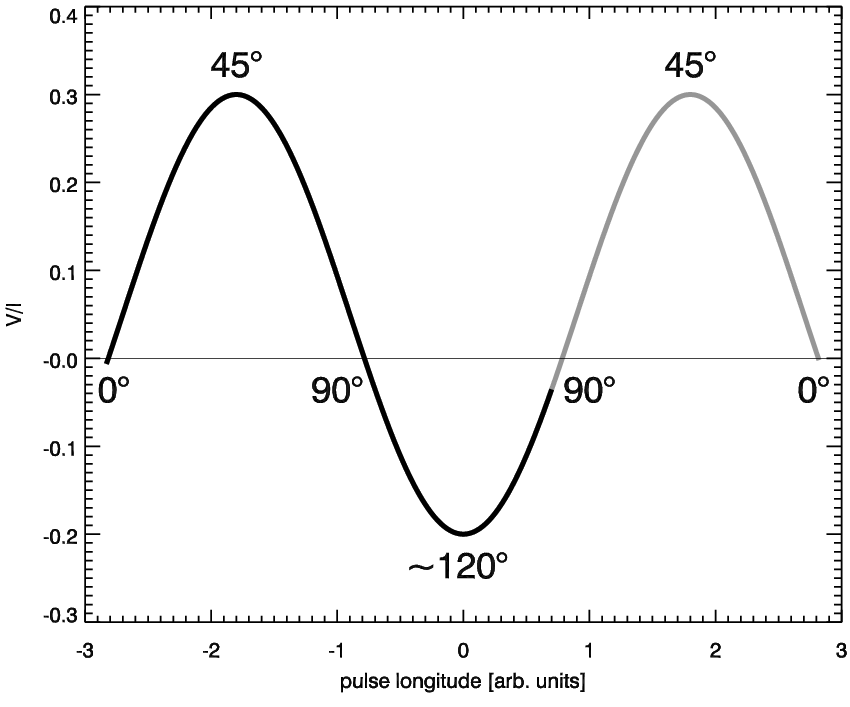
A full derotation of $\psi_{pk}$ back to $0^{\circ}$ would produce a positive $V$ on the right-hand side of the core. This would create a symmetric feature shown in Fig. 19, with two humps of positive $V$ separated by a negative $V$ in the middle. However, in B1237$+$25 the core beam is narrow in comparison to $\Delta_{plr}$ and the right hand side of the $\psi_{pk}(\Phi)$ profile is missing, as implied by Figs. 17b and 18b. Such interpretation is supported by the polarisation profiles of B1541$+$09 at 430 MHz, and B1839$+$09 at 1.4 GHz (see Figs. 8 and 9 in HR10) which exhibit the full symmetric $V$ profile, with the negative $V$ surrounded by the positive maxima of $V$.

The coherent nature of the observed non-RVM PA distortions implies that the incoherent separation of pulsar emission into OPMs, which is based on RVM fits, may not give meaningfull results in the presence of strong PA distortions. Moreover, since the flux ratio of the OPMs mostly reflects the relative magnitude of components of the input polarisation vector (and the width of $N_{\psi,in}$), the intensity profiles of separated OPMs tell little on the OPMs themselves. McKinnon & Stinebring (2000) provide other arguments against the modal separation of profiles.

The complicated loop-like distortions of the core PA are then a result of fast and multiple intermode crossing that occurs when the sightline is passing near the pole, and the projected $B$ field rotates with respect to the PLR basis (which is also rotating). Similar fast variations of $\psi_{pk}$ may be expected when the magnetic field in the radio emission region has a complicated multipolar structure (e.g. Petri 2017).

The CMA model implies that such multipolar distortions of $B$ do not leave a direct imprint of this local $B$ in the observed PA curves. As in the core case, the multipolar $B$ barely changes the illumination of the PLR basis, so the resulting PA distortions appear as transitions between (or departures from) the RVM tracks. These ‘transitional’ distortions are caused by the intermode crossing and reflect the relative orientation of $B$ in the emission and PLR regions, not the absolute direction of $B$ in the multipolar emission region. The numerous distortions of a single PA curve observed in millisecond pulsars (e.g. J0437$-$4715) may be caused by such multipolar $B$.

A rare but striking polarisation effect is presented by pulsars B1919$+$21 (Fig. 18 in MAR15) and B0823$+$26 (Fig. 7 in Everett & Weisberg 2001), in which the PA makes a $45^{\circ}$ jump and follows a continuous PA curve associated with a very weakly polarised emission.

The low $L/I$ suggests that $\psi_{pk}$ is close to $45^{\circ}$ or that $N_{\psi,in}$ is very wide. The first case is shown in Fig. 20, in which $\psi_{pk}=40^{\circ}$ and $\sigma_{\psi,in}=30^{\circ}$. At the profile edges in B1919$+$21, $N_{\Delta\phi}$ must be wide enough to reach the modes at $\Delta\phi=90^{\circ}$, as suggested by the orthogonal PA patches observed at $\Phi\approx-1.5$ in Fig. 18 in MAR15. This is presented in the top panel of Fig. 20, where $\sigma_{\Delta\phi}=90^{\circ}$. Since $N_{\psi,in}$ is not perfectly aligned with $\psi_{pk}=45^{\circ}$, one of the OPM spots is slightly stronger, which defines which OPM is observed as the average PA. In the middle of the profile of B1919$+$21, $N_{\Delta\phi}$ becomes narrower, as shown in the bottom panel of Fig. 20. Therefore, the intrinsic (input) PA distribution (also shown with the line thickness at $\Delta\phi=0$) dominates there. Since $N_{\psi,in}$ peaks near $45^{\circ}$, the average PA offset by $\sim\negthinspace 45^{\circ}$ is observed, and the single pulse samples reveal the variety of incident PAs in the intrinsic $N_{\psi,in}$ distribution. The ‘dirty’, erratic single pulse PA observed in the inner parts of B1919$+$21 profile must then represent the intrinsic (incident) PA, or at least be closer to the intrinsic PA than in the profile edges where the OPMs dominate. Needless to say, the $45^{\circ}$ jumps also appear when $N_{\Delta\phi}$ stays narrow, but moves from $\Delta\phi\sim 0$ to $\sim\negthinspace 90^{\circ}$ (as in Fig. 5).

The transition from the wide to narrow $N_{\Delta\phi}$ should in general be associated with a change of $L/I$ at the $45^{\circ}$ jump. This is because for the wide $N_{\Delta\phi}$ (top in Fig. 20) the two OPM spots of comparable strength produce nearly total depolarisation, whereas for the narrow $N_{\Delta\phi}$ (bottom) $L/I$ has the intrinsic value, which can be large if $N_{\psi,in}$ is narrow. The magnitude of $L/I$ observed on both sides of the $45^{\circ}$ jump in B0823$+$26 (Fig. 7 in Everett & Weisberg 2001, $\Phi=-2^{\circ}$) is indeed very different. If, on the other hand, the incident $N_{\psi,in}$ is wide (and centred close to $45^{\circ}$), then $L/I$ is low on both sides of the $45^{\circ}$ jump. This must be the case of B1919$+$21 which seems to have low $L/I$ both at the edges and in the middle of profile.

References

- Backer (1976) Backer D. C., 1976, ApJ, 209, 895
- Barnard & Arons (1986) Barnard J. J., Arons J., 1986, ApJ, 302, 138
- Beskin & Philippov (2012) Beskin V. S., Philippov A. A., 2012, MNRAS, 425, 814
- Blaskiewicz et al. (1991) Blaskiewicz M., Cordes J. M., Wasserman I., 1991, ApJ, 370, 643
- Cheng & Ruderman (1979) Cheng A. F., Ruderman M. A., 1979, ApJ, 229, 348
- Craig (2014) Craig H. A., 2014, ApJ, 790, 102
- Dyks (2008) Dyks J., 2008, MNRAS, 391, 859
- Dyks (2017) Dyks J., 2017, arXiv:astro-ph/1705.05133
- Dyks et al. (2010) Dyks J., Wright G. A. E., Demorest P., 2010, MNRAS, 405, 509
- Edwards & Stappers (2004) Edwards R. T., Stappers B. W., 2004, A&A, 421, 681
- Everett & Weisberg (2001) Everett J. E., Weisberg J. M., 2001, ApJ, 553, 341
- Gangadhara (2010) Gangadhara R. T., 2010, ApJ, 710, 29
- Gould & Lyne (1998) Gould D. M., Lyne A. G., 1998, MNRAS, 301, 235
- Hankins & Rankin (2010) Hankins T. H., Rankin J. M., 2010, AJ, 139, 168
- Johnston & Weisberg (2006) Johnston S., Weisberg J. M., 2006, MNRAS, 368, 1856
- Karastergiou & Johnston (2006) Karastergiou A., Johnston S., 2006, MNRAS, 365, 353
- Krzeszowski et al. (2009) Krzeszowski K., Mitra D., Gupta Y., Kijak J., Gil J., Acharyya A., 2009, MNRAS, 393, 1617
- Kumar & Gangadhara (2012) Kumar D., Gangadhara R. T., 2012, ApJ, 746, 157
- Lyubarskii & Petrova (1998) Lyubarskii Y. E., Petrova S. A., 1998, Astrophysics and Space Science, 262, 379
- Manchester & Han (2004) Manchester R. N., Han J. L., 2004, ApJ, 609, 354
- McKinnon & Stinebring (2000) McKinnon M. M., Stinebring D. R., 2000, ApJ, 529, 435
- Melrose (2003) Melrose D., 2003, in Bailes M., Nice D. J., Thorsett S. E., eds, Radio Pulsars Vol. 302 of Astronomical Society of the Pacific Conference Series, What Causes the Circular Polarization in Pulsars?. p. 179
- Melrose et al. (2006) Melrose D., Miller A., Karastergiou A., Luo Q., 2006, MNRAS, 365, 638
- Michel (1991) Michel F. C., 1991, Theory of neutron star magnetospheres. University of Chicago Press
- Mitra et al. (2015) Mitra D., Arjunwadkar M., Rankin J. M., 2015, ApJ, 806, 236 (MAR15)
- Mitra & Rankin (2017) Mitra D., Rankin J., 2017, arXiv:astro-ph/1703.09966
- Mitra et al. (2016) Mitra D., Rankin J., Arjunwadkar M., 2016, MNRAS, 460, 3063 (MRA16)
- Mitra & Rankin (2008) Mitra D., Rankin J. M., 2008, MNRAS, 385, 606
- Pétri (2017) Pétri J., 2017, MNRAS, 466, L73
- Petrova & Lyubarskii (2000) Petrova S. A., Lyubarskii Y. E., 2000, A&A, 355, 1168
- Rankin (1983) Rankin J. M., 1983, ApJ, 274, 333
- Rankin & Ramachandran (2003) Rankin J. M., Ramachandran R., 2003, ApJ, 590, 411
- Rybicki & Lightman (1979) Rybicki G. B., Lightman A. P., 1979, Radiative processes in astrophysics. New York, Wiley-Interscience
- Smith et al. (2013) Smith E., Rankin J., Mitra D., 2013, MNRAS, 435, 1984
- Sokolov & Ternov (1968) Sokolov A. A., Ternov I. M., 1968, Synchrotron Radiation. New York: Pergamon
- Stairs et al. (1999) Stairs I. H., Thorsett S. E., Camilo F., 1999, ApJS, 123, 627
- Stinebring et al. (1984) Stinebring D. R., Cordes J. M., Rankin J. M., Weisberg J. M., Boriakoff V., 1984, ApJS, 55, 247
- Tiburzi et al. (2013) Tiburzi C., Johnston S., Bailes M., Bates S. D., Bhat N. D. R., Burgay M., Burke-Spolaor S., Champion D., Coster P., D’Amico N., et al., 2013, MNRAS, 436, 3557
- Wang et al. (2010) Wang C., Lai D., Han J., 2010, MNRAS, 403, 569
- Weisberg & Taylor (2002) Weisberg J. M., Taylor J. H., 2002, ApJ, 576, 942
- Weltevrede & Johnston (2008) Weltevrede P., Johnston S., 2008, MNRAS, 391, 1210
- Xilouris et al. (1998) Xilouris K. M., Kramer M., Jessner A., von Hoensbroech A., Lorimer D. R., Wielebinski R., Wolszczan A., Camilo F., 1998, ApJ, 501, 286
- Young & Rankin (2012) Young S. A. E., Rankin J. M., 2012, MNRAS, 424, 2477