Non-parametric estimation of
Jensen-Shannon Divergence in
Generative Adversarial Network training
Abstract
Generative Adversarial Networks (GANs) have become a widely popular framework for generative modelling of high-dimensional datasets. However their training is well-known to be difficult. This work presents a rigorous statistical analysis of GANs providing straight-forward explanations for common training pathologies such as vanishing gradients. Furthermore, it proposes a new training objective, Kernel GANs, and demonstrates its practical effectiveness on large-scale real-world data sets. A key element in the analysis is the distinction between training with respect to the (unknown) data distribution, and its empirical counterpart. To overcome issues in GAN training, we pursue the idea of smoothing the Jensen-Shannon Divergence (JSD) by incorporating noise in the input distributions of the discriminator. As we show, this effectively leads to an empirical version of the JSD in which the true and the generator densities are replaced by kernel density estimates, which leads to Kernel GANs.
1 INTRODUCTION
Generative Adversarial Networks (GANs), introduced by Goodfellow et al. [9], have become a widely popular framework for generative modeling using deep neural networks. While practitioners find that GANs – particularly for image data – produce sharp and realistic samples, it is well recognized that GANs are difficult to train. Key challenges are: vanishing gradients, local optima leading to mode collapse, high sensitivity to hyperparameters, and finding the right balance between generator and discriminator training in the adversarial set-up (Dinh et al. [5], Goodfellow [8], Goodfellow et al. [10], Metz et al. [21], Radford et al. [24], Salimans et al. [26]).
Various authors have proposed practical modifications of GAN training to address these issues. However, only recently have authors begun to analyze them mathematically and develop principled solutions. An important step in this direction was the work by Arjovsky and Bottou [1], which led to the idea of Wasserstein GANs elaborated in Arjovsky et al. [2] and further developed by Gulrajani et al. [12]. Two important insights were: 1) training the discriminator in GANs till optimality may provably result in vanishing gradients, and 2) the Jensen-Shannon Divergence (JSD) doesn’t yield meaningful information about convergence of distributions if their intersection with the support of the limit-distribution has measure zero. Another important contribution was the work by Metz et al. [21], who proposed to unroll discriminators in the GAN training objective in order to avoid degenerate optima and vanishing gradients.
Our contributions. This work has three major contributions.
- •
First, a rigorous mathematical framework to analyze GANs, which yields a remarkably simple explanation of the vanishing gradient problem.
- •
Second, a novel training objective, Kernel GANs, backed with a principled theoretical analysis along with an empirical study that highlights practical aspects of Kernel GAN training.
- •
Finally, experimentation with different training setups that scale Kernel GANs to large datasets and establish their practical usefulness.
Our rigorous mathematical framework allows us to formulate the results in Arjovsky and Bottou [1] more generally, and it addresses obscurities in the original theory developed in [9]. It appears that a major source of confusion has been the missing distinction between the GAN training objective with respect to the (unknown) target density, and its empirical counterpart used in practical training. This was recently independently pointed out by Arora et al. [3], however, without deriving the implications stated in the present work.
To overcome GAN training pathologies, we analyze approaches for smoothing the JSD in the GAN training objective. We pursue the idea of adding noise terms to the inputs of the discriminator. As we show, this leads to an empirical version of the JSD in which the true and the generator densities are replaced by kernel density estimates. We establish almost sure convergence of this Kernel GAN objective and conditions under which it is asymptotically unbiased.
We support the theoretical analysis with extensive experimentation. Particular emphasis is on understanding the effect of the kernel bandwidth in the training algorithm. We also study the generalization of Kernel GANs by an evaluation of both the fidelity and the diversity of generated samples, also in comparison with baseline methods. Furthermore, we extend the Kernel GAN training setup to enable generative modelling of large-scale real-world datasets.
Related work. In its attempt to establish a rigorous mathematical framework for understanding properties of GANs, this work is related to Arjovsky and Bottou [1]. However, the framework here is more general, e.g., many of the results cover both discrete and continuous distributions, and no parametric family assumptions are imposed on the generators. Moreover we clarify the consequences of working with empirical distributions in practical GAN training, which leads to a remarkably simple explanation of the pathologies discussed in [1]. Plugging kernel density estimates into the objective function bears some similarity with the work by Dziugaite et al. [6], Li et al. [19] and, most recently, [18]. However, these authors optimize generative models with respect to the Maximum Mean Discrepancy (MMD) criterion. Contrastingly, our approach retains the adversarial setup; in fact, it can be regarded as unrolling the discriminator in the GAN training objective till optimality, which is similar in spirit to the methodology proposed by Metz et al. [21].
Outline of this paper. The mathematical framework and theoretical findings are established in Section 2, which also introduces the novel training objective. Section 3 provides practical aspects of training with respect to that objective, and discusses experimental results. Section 4 concludes the paper. Proofs, implementation details and additional experiments are included in the Appendix.
2 THEORETICAL ANALYSIS
2.1 Preliminaries
Let be a probability space. Consider measurable spaces (the output space) and (latent space). Let denote the set of measurable functions (generators), and the set of measurable functions (discriminators). Let be a measure on . For the remainder of this paper, let and be fixed random variable from onto and , respectively. We will make frequent use of the following assumptions:
- (A1)
The distribution of is absolutely continuous with respect to .
- (A2)
For every , the distribution of is absolutely continuous with respect to .
As a consequence, has a -density and has a -density for every . Given iid samples , , …, from the distribution of , our goal is to learn a generator such that for all , or, equivalently, -almost everywhere. The next theorem establishes the existence of such a under the following assumptions:
- (A3)
is a Peano space, i.e., is a compact, connected, and locally connected metric space.
- (A4)
is the support of , i.e., there doesn’t exist an with an open neighborhood in the topology of such that .
Theorem 2.1.
Suppose that (A1)-(A4) hold. Moreover suppose that , is the Borel -algebra on , and is uniformly distributed on . Then there exists a continuous surjection such that for all .
Note that, equivalently, one could have assumed follows any real-valued distribution which is absolutely continuous with respect to the Lebesgue measure. There has been some confusion in the GAN literature about the exact conditions that are required to obtain this result. For example, Goodfellow [8] states the “the only requirements” for to have “full support” on are that the dimension of be “at least as large as the dimension of ”, and be differentiable. This isn’t accurate as may have smaller dimension, as long as its cardinality is not smaller than the one of , and the distribution of is non-atomic. Differentiability of is not required in theory. To obtain an invertible and differentiable mapping , the dimension of must not be smaller than the dimension of . The result in Theorem 2.1 relies on a construction using space-filling curves, which aren’t differentiable.
2.2 GAN Training – Theoretical Case
The GAN approach (Goodfellow et al. [9]) for learning is as follows: for and let
| (1) |
The relation of to density ratio estimation (which becomes apparent in equation (4) below) is discussed in [22]. Intuitively, we wish the discriminator to be close to if is more likely under the distribution of , and close to if is more likely under the distribution of . Hence, the optimal given a fixed generator would attempt to maximize , and the optimal is the one which solves the minmax problem
| (2) |
The following theorem, which generalizes Proposition 1 and Theorem 1 in [9], shows that the max and (arg)min in (2) are well-defined. Note that our formulation neither requires to be differentiable, nor to be continuous.
Theorem 2.2.
Suppose (A1)-(A2) hold. Then
| (3) | |||||
for all and . Hence, for any fixed , any which maximizes has the form
| (4) |
for -almost every , implying that
| (5) | |||||
Assuming that (A3)-(A4) also hold, any generator that minimizes (5) is such that -almost everywhere, and .
The next theorem establishes further properties of the optimal discriminator in (4). It generalizes Theorem 2.1 and 2.2 in [1], which were stated for the special case of and being not-perfectly-aligned submanifolds of .
Theorem 2.3.
Suppose (A1)-(A3) hold. For fixed , let be such that and . Suppose , (where denotes the topological boundary) and . Then the optimal in (4) satisfies and . Moreover, without loss of generality, is continuous -almost everywhere and, in the special case , the gradient exists and for -almost every .
In practice, the discriminator being constant on and poses problems. In particular, when is fixed and is trained till optimality, the gradients may vanish and further updates of become impossible. In their Lemma 1 and 2, Arjovsky and Bottou [1] establish that this is almost surely going to occur whenever the dimension of is smaller than the dimension of , and is parameterized by a standard neural network. As we show next, it is more directly an inevitable consequence of using an empirical version of the objective (1) in practical GAN training.
2.3 GAN Training – Empirical Case
Let be a random variable following the empirical distribution of , …, . By we denote the indicator function which evaluates to if the statement in brackets is true, and to otherwise. Note that, conditionally on , …, , the distribution of is
for , and an analogous statement holds for the distribution of conditional on , …, . It is important to note that practical GAN training (such as in Algorithm 1 in [9]) is not with respect to the theoretical objective (1), but with respect to its empirical counterpart
| (6) |
It appears there has been a wideheld belief among GAN practitioners that optimizing leads to discriminators and generators with the same properties as stated in Theorem 2.3. As the following theorem shows, this isn’t true in general. We add subscripts and to emphasize the dependency of discriminator and generator on the sample size .
Theorem 2.4.
Theorem 2.4 reveals two insights: First, if and both have continuous distributions, then has the same properties as in Theorem 2.3. This suggests the primary reason for vanishing gradients in GAN training is the discrete nature of the empirical objective (6) – which is a remarkably simple explanation.
The second insight is that, when training with respect to (6), there is no theoretical guarantee that -almost everywhere for the optimal generator – which contradicts Proposition 2 in [9]. The only guarantee is that, when applied to , should reproduce the training samples . Note: this does not imply that will solely reproduce training samples; in theory, the samples generated on are arbitrary. Hence, in contrary to the reasoning in [21] and [2], the optimal is not necessarily a Dirac function at the to which assigns the highest values.
In practice, these undesirable properties could be mitigated for the following reasons: 1) the discriminator and generator function spaces and have limited capacity, hence the properties of and may only hold approximately; 2) similarly, alternate training of the generator and discriminator, or not training till optimality could alter the form of and , thereby circumventing pathologies. Limiting the capacity of the networks or finding the right balance between training the generator and discriminator, however, is challenging. This is why GAN training has been regarded as extremely difficult among practitioners.
2.4 Smoothing the Training Objective
A natural approach to avoid the issues pointed out in Theorem 2.3 and Theorem 2.4 is to smooth the Jensen-Shannon Divergence (JSD) in the GAN training objective by adding noise to the input distributions of the optimal discriminator.11 1 This was previously discussed in [1], however, the idea was not pursed beyond an initial analysis. In the following, let be a fixed random variable on which is absolutely continuous with respect to , hence has a -density . We use the following assumption:
- (A5)
In addition to (A3), is a topological group.
This allows us to consider the convolutions and , which are the -densities of and , respectively. The idea is to use, instead of the discriminator in (4), a modified version
| (8) |
If the support of is sufficiently large, then the supports of and will overlap. Hence, it is not possible to construct an optimal with the properties in Theorem 2.3. On the other hand, by the same arguments as in Theorem 2.2, the generator minimizing (8) is such that -almost everywhere, which implies -almost everywhere, i.e. the optimal generator with respect to the theoretical objective still recovers the distribution of . Next, we derive the form of the optimal discriminator for the modified empirical objective.
Theorem 2.5.
Suppose (A1)-(A5) hold and let be fixed. If we replace and in (6) by and , respectively, then the discriminator minimizing the objective has the form
| (9) | |||||
for . Same as in Theorem 2.4, if the cardinality of is greater than or equal to the cardinality of , then any minimizing the objective (6) for is such that .
Note that the smoothing of distributions outlined here is not equivalent to adding noise to the samples , …, or , …, before optimizing the empirical objective, which would lead to the same result as in (7).
As Theorem 2.5 shows, smoothing the empirical distributions and results in an optimal discriminator which, if the support of is sufficiently large, won’t cause vanishing gradients. However, there is still no guarantee that the optimal generator recovers the distribution of apart from reproducing training samples. In the following section we discuss a new training objective which addresses this issue.
2.5 Kernel GANs
Throughout the rest of the paper we assume , is absolutely continuous with respect to the Lebesgue measure on , , and for some . Moreover, we assume that is parameterized by . We write for the generator parameterized by , and for the density of .
It is instructive to note the resemblance of the optimal discriminator in (9) with a ratio of kernel densities: Let be a measurable, bounded and square-integrable function (kernel), and (bandwidth). For consider the kernel density estimates
| (10) | |||||
| (11) |
of and . Choosing , we can regard (9) as a kernel estimate of the density ratio . Our key idea is to plug the optimal discriminator (9) back into the empirical training objective (6), i.e., consider with . This results in the Kernel GAN training objective:
| (12) |
where is a regularizer to avoid underflow issues. In contrast to conventional GAN training, only the generator is explicitly updated when optimizing (12). The discriminator is updated implicitly through changes in the density estimates (11). Note that plugging the optimal discriminator in (9) into the training objective (6) can be regarded as unrolling the discriminator same as in Metz et al. [21], where in our case the discriminator is unrolled to closed-form optimality.
The following theorem establishes convergence of the objective (12).
Theorem 2.6.
Suppose (A1)-(A5) hold. Moreover, suppose and are bounded and uniformly continuous for all , and has compact support and is of the form , where is a polynomial and a bounded non-negative function with bounded variation. Let be a sequence asymptotically equivalent to for some finite constant and . Then
| (13) |
-almost surely for all and .
The regularizer is required for establishing the convergence in (13). It results in estimates of the theoretical JSD that are asymptotically biased. In particular, while converges to (which is the minimum value of JSD) if is such that , it may converge to smaller values for other values of . Hence, minimizing would not result in a generator recovering (although can be chosen arbitrarily small, hence the practical difference might be negligible). However, as we show in Appendix A.2, if , then can be modified such that its limit is minimized by a recovering the distribution of .
3 EXPERIMENTS
In this section, we discuss practical learning of Kernel GANs. First, we demonstrate the learning on small and mid-sized datasets – a Mixture-of-Gaussian (MOG) toy dataset ([21]) and MNIST ([16]). Further, we study the effect of kernel bandwidth along with practical approaches such as generating in a lower-dimensional feature space that is independently learned using an autoencoder.
Second, we establish practical usefulness of Kernel GANs by scaling them to two high-dimensional datasets: CIFAR-10 ([15]) and CelebA ([20]). We enable this with a modified training setup that involves kernel learning, similar to [18].
Finally, we conduct various evalutions of the performance of the trained generators. In a quantitative evaluation, we compare Kernel GANs with MMD-based models (Li et al. [19], Dziugaite et al. [6], Li et al. [18]), which also use kernel-based statistics, but in a non-adversarial fashion. Full details on the implementation and all the experiments can be found in Appendix A.3 and A.4.
3.1 Learning Kernel GANs
Algorithm 1 outlines our general training protocol for learning the generator parameters that minimize the training objective (12).
Hyperparameters.
Previously, Li et al. [19] and Dziugaite et al. [6] used RBF kernels in their training objectives for generative models. While [19] deploys a mixture of RBF kernels, [6] uses Bayesian Optimisation to determine a suitable bandwidth. Moreover, both works suggest to use the median-trick (Gretton et al. [11]) as a method to choose kernel bandwidths for computing MMD statistics. Intuitively, small bandwidths push the generator towards producing samples that are similar to the training set. However, initial bandwidths that are too small will not give gradients in areas that are far from the modes of the training set. We therefore explored gradual reductions of the bandwidth during training, similar to cooling schedules in simulated annealing (e.g., Hajek [13], Nourani and Andresen [23]). While the regularizer is required for deriving Theorem 2.6, we didn’t find it to play a crucial role in the practical experiments and therefore set it equal to zero. A further investigation of the practical effect of will be part of future work.
MOG Toy Dataset.
For the MOG dataset, was a 100-dimensional standard normal distribution, and the generator used was a three-layer fully connected network (128-relu-128-relu-128-tanh). Figure 1 shows the evolution of the generator during the training, as the bandwidth is gradually decreased. Initially the generated samples are dispersed randomly. As the bandwidth is decreased, they begin to concentrate around the modes of the MOG distribution.

MNIST.
We succesfully trained three different generative models for MNIST. Two of these were trained to sample directly in the space of greyscale images. The third model used an autoencoder to map the images onto a lower-dimensional feature space, in which the generator was trained.
The three models used following architectures: a fully connected network (FC); a deconvolutional network with batch normalisation (DC); a fully connected network for the feature space (FC-FS). We adopted the architectures proposed in [19] for FC and FC-FS, and the architecture proposed in [24] for DC. As latent variable , all models used samples from a 10-dimensional uniform distribution. We used a mixture of RBF kernels for training these models (see the appendix for details). For FC-FS, we also experimented with different bandwidths in simple RBF kernels.
Generated samples from FC, DC and FC-FS are shown in Figure 2 (a)-(c). We found that samples from FC-FS had a very smooth appearance. DC generated sharper samples than FC, but still produced some artifacts. The sharpness of the FC-FS samples with simple RBF kernels and different bandwidths is evaluated in the appendix. Quantitative measures of sample fidelity and diversity are discussed below.
We observed that training randomly initialized networks can be numerically unstable for very small bandwidths, leading to artifacts in the produced images. For very large bandwidths, we occasionally found the generator to collapse and produce undesired samples like mean images. We noticed, however, that the generator model recovered when we increased or decreased the bandwidth appropriately in subsequent training iterations. An analysis is provided in the appendix. This suggests that kernel bandwidths can be used as “knobs” for correcting over- or underfitting of generative models during the training process.
| FC | DC | FC-FS | GMMN-AE | GMMN | MNIST Test | |
|---|---|---|---|---|---|---|
| EE | 0.408 | 0.289 | 0.365 | 0.361 | 0.293 | 0.023 |
| ENN | 23.005 | 20.713 | 14.674 | 14.730 | 27.852 | 19.299 |
| LS | 6.601 | 7.464 | 6.916 | 6.948 | 7.408 | 9.752 |
| JSD | -1.384 | -1.385 | -1.371 | -1.372 | -1.383 | -1.386 |
| JSD-F | -0.740 | -0.740 | -0.769 | -0.776 | -0.689 | -0.693 |
| JSD-S | -0.644 | -0.645 | -0.603 | -0.596 | -0.694 | -0.693 |
| MMD | 0.019 | 0.017 | 0.084 | 0.091 | 0.005 | 0.000 |
3.2 Scaling Kernel GANs
Although being sufficient in theory, we found it difficult to train Kernel GANs for colored images using plain RBF kernels. To impose more structure in kernel-based training of generative models, [19] had suggested to use convolutional autoencoders to learn a lower dimensional feature space for colored images. [18] used this approach for training GMMN models on colored images both in feature and data space, however they observed quality issues in the generated samples. Instead they pursued an alternative approach where, much like a GAN setup, they learn a network which transforms the original space into a lower dimensional space over which the kernel is computed. We adopt their approach, leading to a modified Kernel GAN training objective, , which is the same as (12), except that the kernels operate on the space instead of :
| (14) | |||
| (15) |
The parameters are learned in a min-max fashion: . Similar to conventional GAN training, and are optimized alternatingly. In practice, we observed that additional regularization was required for stable learning. We used the experimental setup of [18], which models the function as the encoder of an autoencoder and regularizes the objective function with the autoencoder reconstruction loss.
CIFAR10 and CelebA.
We used this setup to successfully train Kernel GANs for the CIFAR10 and CelebA datasets. We adopted and appropriately rescaled hyperparameters and regularization weights of [18]. We trained a Deep Convolutional architecture for both datasets. The dimension of the encoded space was fixed to 100. While CIFAR10 was trained with a 128-dimensional standard normal distribution for , CelebA was trained with a 64-dimensional . Samples obtained from the trained generators are shown in Figure 3. We found that they were qualitatively comparable to the results in [18].
3.3 Quantitative Evaluation
MNIST.
Quantifying the performance of generative networks – particularly their ability to generalize and produce diverse samples – remains a challenging task ([28, 31]). In this paper, we report the following metrics:
Expected entropy (EE): As proposed in [26], we trained a probabilistic classifier (LeNet [17]) and computed the expected entropy of the classifier probabilities for samples . For all metrics, we used Monte-Carlo estimates of expected values, based on 10,000 samples from . Expected nearest-neighbour distance (ENN): To assess the similarity of generated samples with samples in the training set, we determined the expected value of the Euclidean distance between samples from and their nearest neighbor in the train set. LeNet score (LS): Similar to the Inception score proposed in [26], we computed the exponential of the expected Kullback-Leibler divergence between the predicted class probabilities for samples , and the frequency of classes (=digits) in the MNIST train set. Jensen-Shannon divergence (JSD): We estimated the JSD between the unknown data distributions and by computing (12) over the MNIST test set and samples produced by . We also report the corresponding values JSD-F and JSD-S of the first and second term in (12). Maximum Mean Discrepancy (MMD): Finally, we also report the MMD statistic ([11]).
Table 1 shows a comparison of different generators. GMMN and GMMN-AE are the data- and code-space Generative Moment Matching Networks (GMMN) proposed in [19]. The numbers in the MNIST Test column are obtained by using the MNIST test set instead of generated samples; hence they can be regarded as the performance of an ideal generator, with optimal trade-off between fidelity (EE), diversity (ENN, LS), and overall consistency (JSD). In this regard, we found DC performed the best among all trained generators: it achieved the lowest EE, comparable ENN, and the closest LS in comparison with MNIST Test. FC-FS and GMMN-AE also achieved high fidelity, but seemed to exhibit less diversity. Interestingly, the first and second term of the JSD were observed to be imbalanced for these models. We hypothesize that keeping JSD-F and JSD-S balanced during training is key to obtaining generators with good generalization capacity.
CIFAR10.
We computed the Inception score ([26]) mean and standard deviation for 5 10k samples obtained from a Kernel GAN that was trained for 5,000 iterations. The score for held-out CIFAR10 images (which can be regarded as gold standard) was 11.95 ( .20). Kernel GANs yielded a score of 4.22 ( .02), which is significantly higher than the scores for GMMN-AE and GMMN (3.94 .04 and 3.47 .03, respectively), but lower than for MMD-GAN (6.17 .07, see [18]). The latter finding can be explained by the fact that we did not optimize hyperparameters and regularization weights for Kernel GANs, which could lead to further improvements in future work.
4 CONCLUSIONS
We established a rigorous framework for analyzing statistical properties of Generative Adversarial Network training. To overcome potential pathologies (in particular, vanishing gradients), we introduced a novel training objective, which can be regarded as minimizing a non-parametric estimate of the Jensen-Shannon Divergence. We analyzed its asymptotic properties and showed its practical applicability.
We see several directions for future work: 1) Advance the design of optimal kernels and strategies for annealing the bandwidths. 2) Further analyze statistical properties of the proposed training objective, in particular, the effect of the regularizer. 3) Investigate the effect of imbalances between the first and second term in the training objective; we believe this could lead to the design of adaptive training protocols which ensure both fidelity and diversity of generator samples.
References
- [1] M. Arjovsky and L. Bottou. Towards principled methods for training generative adversarial networks. arXiv preprint arXiv:1701.04862, 2017.
- [2] M. Arjovsky, S. Chintala, and L. Bottou. Wasserstein gan. arXiv preprint arXiv:1701.07875, 2017.
- [3] S. Arora, R. Ge, Y. Liang, T. Ma, and Y. Zhang. Generalization and equilibrium in generative adversarial nets (gans). arXiv preprint arXiv:1703.00573v2, 2017.
- [4] V. I. Bogachev. Measure Theory. Springer Verlag, Berlin, 2007.
- [5] L. Dinh, J. Sohl-Dickstein, and S. Bengion. Density estimation using real nvp. arXiv preprint arXiv:1605.08803, 2016.
- [6] G. K. Dziugaite, D. M. Roy, and Z. Ghahramani. Training generative neural networks via maximum mean discrepancy optimization. In Proceedings of the Thirty-First Conference on Uncertainty in Artificial Intelligence, UAI’15, pages 258–267, Arlington, Virginia, United States, 2015. AUAI Press. ISBN 978-0-9966431-0-8. URL http://dl.acm.org/citation.cfm?id=3020847.3020875.
- [7] E. Giné and A. Guillou. Rates of strong uniform consistency for multivariate kernel density estimators. Annales de l’Insitut Henri Poincaré, 38(6):907–921, 2002.
- [8] I. Goodfellow. Nips 2016 tutorial: Generative adversarial networks. arXiv preprint arXiv:1701.00160, 2016.
- [9] I. Goodfellow, J. Pouget-Abadie, M. Mirza, B. Xu, D. Wade-Farley, S. Ozair, and A. Courville. Generative adversarial nets. Advances in Neural Information Processing Systems, 27:2672–2680, 2014a.
- [10] I. Goodfellow, J. Shlens, and C. Szegedy. Explaining and harnessing adversarial examples. arXiv preprint arXiv:1412.6572, 2014b.
- [11] A. Gretton, K. M. Borgwardt, M. J. Rasch, B. Schölkopf, and A. Smola. A kernel two-sample test. Journal of Machine Learning Research, 13(Mar):723–773, 2012.
- [12] I. Gulrajani, F. Ahmed, M. Arjovsky, V. Dumoulin, and A. Courville. Improved training of wasserstein gans. arXiv preprint arXiv:1704.00028v1, 2017.
- [13] B. Hajek. Cooling schedules for optimal annealing. Mathematics of Operations Research, 13(2):311–329, 1988.
- [14] D. Kingma and J. Ba. Adam: A method for stochastic optimization. arXiv preprint arXiv:1412.6980, 2014.
- [15] A. Krizhevsky and G. Hinton. Learning multiple layers of features from tiny images. Technical report, University of Toronto, 2009.
- [16] Y. LeCun, L. Bottou, Y. Bengio, and P. Haffner. Gradient-based learning applied to document recognition. Proceedings of the IEEE, 86(11):2278–2324, 1998.
- [17] Y. LeCun et al. Lenet-5, convolutional neural networks.
- [18] C.-L. Li, W.-C. Chang, Y. Cheng, Y. Yang, and B. Póczos. Mmd gan: Towards deeper understanding of moment matching network. arXiv preprint arXiv:1705.08584, 2017.
- [19] Y. Li, K. Swersky, and R. S. Zemel. Generative moment matching networks. In ICML, pages 1718–1727, 2015.
- [20] Z. Liu, P. Luo, X. Wang, and X. Tang. Deep learning face attributes in the wild. CVPR, pages 3730–3738, 2015.
- [21] L. Metz, B. Poole, D. Pfau, and J. Sohl-Dickstein. Unrolled generative adversarial networks. arXiv preprint arXiv:1611.02163, 2016.
- [22] S. Mohamed and B. Lakshminarayanan. Learning in implicit generative models. arXiv preprint arXiv:1610.03483v4, 2016.
- [23] Y. Nourani and B. Andresen. A comparison of simulated annealing cooling strategies. J. Phys. A: Math. Gen., 31:8373–8385, 1998.
- [24] A. Radford, L. Metz, and S. Chintala. Unsupervised representation learning with deep convolutional generative adversarial networks. arXiv preprint arXiv:1511.06434, 2015a.
- [25] A. Radford, L. Metz, and S. Chintala. Unsupervised representation learning with deep convolutional generative adversarial networks. arXiv preprint arXiv:1511.06434, 2015b.
- [26] T. Salimans, I. Goodfellow, W. Zaremba, V. Cheung, A. Radford, and X. Chen. Improved techniques for training gans. Advances in Neural Information Processing Systems, 29:2226–2234, 2016.
- [27] A. H. Schoenfeld. Continuous measure-preserving maps onto peano spaces. Pacific Journal of Mathematics, 58(2):627–642, 1975.
- [28] L. Theis, A. V. D. Oord, and M. Bethge. A note on the evaluation of generative models. arXiv preprint arXiv:1511.01844, 2015.
- [29] T. Tieleman and G. Hinton. Lecture 6.5-rmsprop: Divide the gradient by a running average of its recent magnitude. COURSERA: Neural networks for machine learning, 4(2), 2012.
- [30] S. Willard. General Topology. Dover Publications, Mineola, New York, 1970.
- [31] Y. Wu, Y. Burda, R. Salakhutdinov, and R. Grosse. On the quantitative analysis of decoder-based generative models. 5th International Conference on Learning Representations, 2017.
A.1: Proofs
Proof of Theorem 2.1:
This is an immediate consequence of Theorem 1 in Schoenfeld [27], which builds on the classical result from Hahn-Mazurkiewicz that a metric space is the continuous image of the unit interval if and only if the space is compact, connected and locally connected.
Proof of Theorem 2.2:
The arguments are analogous to the proofs of Proposition 1 and Theorem 1 in Goodfellow et al. [9], using the change-of-variable formula for general pushforward measures (Bogachev [4]).
Proof of Theorem 2.3:
This is an immediate consequence of Urysohn’s Lemma (Section 15 in Willard [30]), and the assumption that is a compact Hausdorff space.
Proof of Theorem 2.4:
We first note that
where denotes the counting measure on , and and the -densities of conditional on , …, , and of conditional on , …, , respectively:
| and | (16) |
for . Hence, completely analogous to Theorem 2.2, we obtain that any maximizing has the form
for , and hence the result in (7) follows. Again completely analogous to Theorem 2.2, any generator minimizing the objective (6) for is such that for all , which holds if and only if .
Proof of Theorem 2.5:
Proof of Theorem 2.6:
Let and be fixed. First we note that the kernel , the densities , and the sequence satisfy conditions (K2), (D2), (W2) in Giné and Guillou [7]. Consequently, by Theorem 3.3 in [7],
-almost surely. Since is uniformly continuous and has compact support, it is easy to obtain from equation (1.3) in [7]:
Consequently, by the triangle inequality,
| (17) |
-almost surely. Using the same arguments, we obtain
| (18) |
-almost surely. Now let denote a finite upper bound both for and (which exists by our assumptions). Note that is uniformly continuous on . Hence, with (17) and (18), we obtain
-almost surely. Consequently,
| (19) |
-almost surely. Moreover, by the Strong Law of Large Numbers,
| (20) |
-almost surely. Hence, using (19), (20) and the triangle inequality, we obtain
-almost surely which is the desired result for the first term in (13). The result for the second term follows by analogous arguments, which proves the theorem.
A.2: Asymptotically unbiased estimation of
In order to establish , introduce the following function of and :
Note that is the Jensen-Shannon Divergence (multiplied by ) between the densities
| and |
Hence, is minimized for such that -almost everywhere, which is equivalent to -almost everywhere. Next, observe that is equal to the right-hand side in (13), plus the following two terms:
Now suppose , , …are sampled independently according to the probability density , and consider the estimators
Under the same assumptions as in Theorem 2.6, we obtain
-almost surely. Hence, converges to a limit which is minimized by such that the generator recovers .
A.3: Implementation details
MNIST Autoencoder. The autoencoder for Feasture Space (FS) based Kernel GANs of MNIST were trained to yield 32-dimensional feature vectors of images, as suggested in [19]. The architecture used was: 784-1024-sigmoid-32-sigmoid-32-sigmoid-1024-sigmoid-784. The model was trained with cross-entropy as the reconstruction loss, dropouts in the encoder layers, and Adam [14] for optimization.
MNIST Generators. The achitectures used for the generators were:
Training was performed with a minibatch size of (cf Algorithm 1), and RMSProp [29] (learning rate of 0.001) for optimization.
Classifier for LeNet score. A LeNet-like classifier was trained with the following architecture: (28,28,1)-conv(32,(3,3))-relu-maxpool(2,2)-conv(64,(3,3))-relu-maxpool(2,2)-fc(128)-relu-10-softmax. Training was performed using Adam and with dropout for regularization.
Generative Moment Matching Networks. We trained the data-space and code-space networks of [19], which they define as GMMN and GMMN-AE respectively. We used a mixture of RBF kernels (GMMN: , GMMN-AE: ).
CIFAR10 and CelebA. We trained models based on DCGAN ([25]) architecture for both CIFAR10 and CelebA. Similar to [18], we trained a network for which was modelled as an encoder of a convolutional autoencoder. The encoding dimension was fixed to 100. A mixture of RBF kernels () was used as kernels in equation 12. As mentioned in section 3.2, training of was regularised with autoencoder reconstruction loss (with a weight of 100). Additionally, the weights of the network were clipped to a range of after every update. This setup was identitical to the one used in [18]22 2 https://github.com/OctoberChang/MMD-GAN. For computing Inception Score, we used the script provided in the work of [12] 33 3 https://github.com/igul222/improved_wgan_training/blob/master/tflib/inception_score.py
Hyperparameters including the model architecture, values of kernel bandwidth were not optimised for any of the experiments. Further, we also believe that longer schedules for optimisation can affect the performance of generators.
A.4: Experiments
MNIST generated samples. Figure 6–8 show the generator samples for MNIST. For comparison, we include a sample from the MNIST test set in Figure 8.

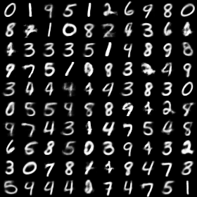


Effect of the kernel bandwidth. We conducted experiments with the FC-FS architecture and simple RBF kernels with different bandwidths. Figure 8 shows samples generated for the MNIST dataset. As can be seen, the sample quality is comparable to FC-FS, however, some digits appear to be over- and under-represented, respectively. Table 2 shows the EE and EEN metrics for on the MNIST dataset for different bandwidths. We note that smaller bandwidths result in generator samples with lower EE. Below we show EE values for samples generated over 2-dimensional manifolds in the latent space, illustrating that lower EE stems both from generated samples with higher visual fidelity, and sharper transitions between low-entropy regions in the latent space. Similarly, also the EEN values decrease with the bandwidth. This can be regarded as a loss of diversity, as generated samples become more and more similar to instances in the training set.
| sum-RBF | |||||||
|---|---|---|---|---|---|---|---|
| EE | 2.117 | 1.388 | 1.096 | 1.079 | 0.783 | 0.406 | 0.365 |
| ENN | 28.973 | 21.075 | 18.268 | 17.295 | 16.272 | 15.378 | 14.730 |
We observed that, for very large values of the kernel bandwidth , the generated samples have a tendency to collapse to the mean of the training instances. Figure 9 analyzes the behaviour of the training objective in (12) as a function of . We compare two different generators: an “ideal” one (black line), which is able – given 100 samples from the MNIST training set, to produce 100 different samples. The red line shows objective function values of a generator which simply produces the mean of the 100 training samples. As can be seen in (a), for large values of the latter generator performs better with regard to the training objective. For small values, the order is reverse. Interestingly, for large the objective function values of the generator producing the mean is below . As (b) and (c) show, this is due to a large imbalance of the first and second term in the training objective. Hence, we hypothesize that the training of meaningful generators should not only aim to minimize (12), but also aim to keep the first and second term in (12) balanced. A deeper investigation of the trade-off between these two terms will be future work.
Entropy carpets. Given a trained GAN and points , in the latent space , it is often instructive to inspect the generated images for . Recently, Dinh et al. [5] proposed an angle-based 2-dimensional manifold interpolation between four points . Here we explore more conventional convex combinations, given by
In practice, we let and vary along a mesh grid of a unit-length square. Figure 10-12 display the image manifolds generated by three different models, along with the “entropy carpets” which show the entropy of a probabilistic classifier (we use LeNet, see above) at each point of the manifold. Bright colors correspond to high-entropy regions, dark colors to low entropy. Entropy carpets can be regarded as a semi-qualitative-semi-quantitative way to relate the manifolds of generated images to the Expected Entropy (EE) metric reported in Tables 2 and 1. Of particular interest are the inter-digit transitions which coincide with high entropy. Typically, the output of the generator is uninterpretable in those regions. Hence, an ideal generator should have as few and as sharp transitions between different modes as possible.


Figures 15-15 show the entropy carpets for the FC-FS model trained with bandwidths . Beyond the Expected Entropy metrics reported in Tables 2, the entropy carpets give an idea of the fraction of points that result in meaningful versus non-meaningful images. Interestingly, even for , significant parts of result in high-fidelity images; however, there are large areas in between the modes in which the generator only generates “noise” from the point-of-view of the classifier. .


