The Lieb–Liniger model [18, 19] describes a system of $N$ indistinguishable bosons subject to a delta-function interaction potential in a one-dimensional geometry. The Hamiltonian is

$$\hat{H}=-\sum_{i=1}^{N}\frac{\partial^{2}}{\partial x^{2}_{i}}+2c\sum_{i<j}^{N}\delta(x_{i}-x_{j}),$$

(1)

where $c$ is the interaction strength, and we have set $\hbar=1$ and the particle mass $m=1/2$. The interactions are attractive for $c<0$, and repulsive for $c>0$. The eigenstates of Hamiltonian (1) in the ordered spatial permutation sector $R_{p}$ ($x_{1}\leq x_{2}\leq\dots\leq x_{N}$) are given by the coordinate Bethe ansatz in the form [22]

	$\displaystyle\zeta_{\{\lambda_{j}\}}(\{x_{i}\})$	$\displaystyle\equiv\langle\{x_{i}\}|\{\lambda_{j}\}\rangle$
		$\displaystyle=\,A_{\{\lambda_{j}\}}\sum_{\sigma}(-1)^{[\sigma]}\;a(\sigma)\;\mathrm{exp}\Big[i\sum_{m=1}^{N}x_{m}\lambda_{\sigma(m)}\Big],$		(2)

where the sum runs over all permutations $\sigma=\{\sigma(1),\sigma(2),\cdots,\sigma(N)\}$ of $\{1,2,\cdots,N\}$, $(-1)^{[\sigma]}$ denotes the sign of the permutation, and the scattering factors are

$$a(\sigma)=\prod_{k>l}\left(\lambda_{\sigma(k)}-\lambda_{\sigma(l)}-ic\right).$$

(3)

The quantities $\lambda_{j}$ are termed the rapidities, or quasimomenta of the Bethe-ansatz wave function. The normalization constant $A_{\{\lambda_{j}\}}$ is given by [22]

$$A_{\{\lambda_{j}\}}=\big[N!\;\mathrm{det}\{M_{\{\lambda_{j}\}}\}\;\prod_{k>l}[(\lambda_{k}-\lambda_{l})^{2}+c^{2}]\big]^{-1/2}\;,$$

(4)

where $M_{\{\lambda_{j}\}}$ is the $N\times N$ matrix with elements

	$\displaystyle[M_{\{\lambda_{j}\}}]_{kl}$	$\displaystyle=\delta_{kl}\Big(L+\sum_{m=1}^{N}\frac{2c}{c^{2}+(\lambda_{k}-\lambda_{m})^{2}}\Big)$
		$\displaystyle\qquad-\frac{2c}{c^{2}+(\lambda_{k}-\lambda_{l})^{2}}.$		(5)

Imposing periodic boundary conditions leads to a set of $N$ equations for the $N$ rapidities, the so-called Bethe equations

$$e^{iL\lambda_{j}}=\prod_{l\neq j}\frac{(\lambda_{j}-\lambda_{l})+ic}{(\lambda_{j}-\lambda_{l})-ic}\;,$$

(6)

where $L$ is the length of the periodic geometry. The rapidities determine the total momentum $P=\sum_{j=1}^{N}\lambda_{j}$ and energy $E=\sum_{j=1}^{N}\lambda_{j}^{2}$ of the system in each eigenstate. The ground state of the system for attractive interactions is an $N$–body bound state (the finite-system analogue of the McGuire cluster state [37]) and has purely imaginary rapidities [38, 39]. All eigenstates corresponding to bound states have some Bethe rapidities with imaginary components. This is in contrast to the repulsively interacting system ($c>0$), for which the solutions $\{\lambda_{j}\}$ to the Bethe equations (6) are purely real. These are usually parameterized by a set of quantum numbers $\{m_{j}\}$, which for $c\rightarrow+\infty$ are proportional to $\{\lambda_{j}\}$, see e.g. Ref. [22]. For the attractively interacting gas, it is more convenient to enumerate the solutions of the Bethe equations (6) by their corresponding $N$ ideal-gas (i.e., $c=0$) quantum numbers $\{n_{j}\}$, where $k_{j}=2\pi n_{j}/L$ are the quantized free single-particle momenta in the finite ring and $n_{j}$ is an integer²² 2 The energy of an eigenstate with $\{n_{j}\}$ for $c\rightarrow 0^{-}$ connects to the energy of the eigenstate with $\{m_{j}^{(0)}+n_{j}\}$ for $c\rightarrow 0^{+}$. Here, $\{m_{j}^{(0)}\}$ are the quantum numbers of the “Fermi-sea” ground state for $c>0$. In the remainder of this article, we will label states of the repulsive gas by their reduced quantum numbers $\{n_{j}\}\equiv\{m_{j}-m_{j}^{(0)}\}$. [39]. In this paper, in which we consider ground-state correlations and quenches from the ideal-gas ground state, we only need to consider eigenstates that are parity invariant, i.e., those for which we can order the $n_{j}$ such that $n_{j}=-n_{N+1-j}$ for $j\in[1,N]$. Thus, we can label all eigenstates by $\lfloor N/2\rfloor$ quantum numbers $\{n_{j}\}$, where $\lfloor\dots\rfloor$ is the floor function. By convention we choose these numbers to be the nonnegative values $\{n_{j}\}$, which we regard as sorted in descending order (for odd $N$, $n_{(N+1)/2}=0$).

Our results depend explicitly on the number of particles $N$ in our system, though the extent $L$ of our periodic geometry, and consequently the density $n\equiv N/L$ of the gas, is arbitrary. We follow Refs. [18, 19] in absorbing the density into the dimensionless interaction-strength parameter $\gamma=c/n$. Our finite-sized system is then identified by the specification of both $\gamma$ and $N$. The Fermi momentum $k_{F}=(2\pi/L)(N-1)/2$, which is the magnitude of the largest rapidity in the ground state in the Tonks–Girardeau limit of infinitely strong repulsive interactions [22], is a convenient unit of inverse length and so we specify lengths in units of $k_{F}^{-1}$, energies in units of $k_{F}^{2}$, and times in units of $k_{F}^{-2}$.

The static and dynamic behaviour of the Lieb-Liniger gas can be characterized by the normalized $m^{\mathrm{th}}$-order correlation functions

$\displaystyle g^{(m)}$

$\displaystyle(x_{1},\dots,x_{m},x_{1}^{\prime},\dots,x_{m}^{\prime};t)\equiv\frac{\left\langle\hat{\Psi}^{\dagger}(x_{1})\cdots\hat{\Psi}^{\dagger}(x_{m})\hat{\Psi}(x_{1}^{\prime})\cdots\hat{\Psi}(x_{m}^{\prime})\right\rangle}{\left[\langle\hat{n}(x_{1})\rangle\cdots\langle\hat{n}(x_{m})\rangle\langle\hat{n}(x_{1}^{\prime})\rangle\cdots\langle\hat{n}(x_{m}^{\prime})\rangle\right]^{1/2}},$

(7)

where $\hat{\Psi}^{(\dagger)}(x)$ is the annihilation (creation) operator for the Bose field, $\hat{n}(x)\equiv\hat{\Psi}^{\dagger}(x)\hat{\Psi}(x)$ is the particle-density operator, and $\langle\cdots\rangle\equiv\mathrm{Tr}\{\hat{\rho}(t)\cdots\}$ denotes an expectation value with respect to a Schrödinger-picture density matrix $\hat{\rho}(t)$. Due to the translational invariance of the system the density is constant [i.e., $\langle\hat{n}(x)\rangle\equiv n$] and the correlation functions are invariant under global coordinate shifts $x\to x+d$. Without loss of generality, we therefore set one of the spatial coordinates to zero and focus on the first-order correlation function $g^{(1)}(x)\equiv g^{(1)}(0,x)$, the second-order correlation function $g^{(2)}(x)\equiv g^{(2)}(0,x,x,0)$, and the local third-order correlation $g^{(3)}(0)\equiv\langle[\hat{\Psi}^{\dagger}(0)]^{3}[\hat{\Psi}(0)]^{3}\rangle/n^{3}$. We also consider the momentum distribution

$$\widetilde{n}(k)=n\int_{0}^{L}dx\;e^{-ikx}g^{(1)}(x),$$

(8)

which we evaluate at the discrete momenta $k_{j}$.

For a system in a pure state $|\psi(t)\rangle$, Eq. (7) reads

		$\displaystyle g^{(m)}(x_{1},\dots,x_{m},x_{1}^{\prime},\dots,x_{m}^{\prime};t)=\frac{1}{n^{m}}\langle\psi(t)|\hat{\Psi}^{\dagger}(x_{1})\cdots\hat{\Psi}^{\dagger}(x_{m})\hat{\Psi}(x_{1}^{\prime})\cdots\hat{\Psi}(x_{m}^{\prime})|\psi(t)\rangle,$
		$\displaystyle=N!\!\int_{0}^{L}\!\frac{dx_{m+1}\cdots dx_{N}}{n^{m}(N-m)!}\psi^{*}(x_{1},\dots,x_{m},x_{m+1},\dots,x_{N},t)\psi(x_{1}^{\prime},\dots,x_{m}^{\prime},x_{m+1},\dots,x_{N},t)\,.$		(9)

By expressing the wave function $\psi(\{x_{j}\},t)$ in terms of Lieb–Liniger eigenstates $\zeta_{\{\lambda_{j}\}}(\{x_{i}\})$ [Eq. (2)], we can calculate the integrals in Eq. (9) semi-analytically with the methodology of Ref. [33]. This approach also allows for the evaluation of the overlaps of the initial state with Lieb–Liniger eigenstates necessary for our nonequilibrium calculations in Sec. 4³³ 3 We note that direct evaluation of the normalization constant $A_{\{\lambda_{j}\}}$ via Eq. (4) is susceptible to catastrophic cancellations similar to those discussed in Appendix B. In practice, we therefore obtain the constants $A_{\{\lambda_{j}\}}$ by evaluating the self-overlaps of unnormalized Bethe eigenfunctions using the methodology of Ref. [33].. In Sec. 5, we consider the relaxed state of the system, as described by the diagonal-ensemble [73] density matrix $\hat{\rho}_{\mathrm{DE}}\equiv\sum_{\{\lambda_{j}\}}\rho^{\mathrm{DE}}_{\{\lambda_{j}\}}|\{\lambda_{j}\}\rangle\langle\{\lambda_{j}\}|$, for which Eq. (7) reads

		$\displaystyle g_{\mathrm{DE}}^{(m)}(x_{1},\dots,x_{m},x_{1}^{\prime},\dots,x_{m}^{\prime})=\frac{1}{n^{m}}\mathrm{Tr}\{\hat{\rho}_{\mathrm{DE}}\hat{\Psi}^{\dagger}(x_{1})\cdots\hat{\Psi}^{\dagger}(x_{m})\hat{\Psi}(x_{1}^{\prime})\cdots\hat{\Psi}(x_{m}^{\prime})\},$
		$\displaystyle=\frac{1}{n^{m}}\sum_{\{\lambda_{j}\}}\rho^{\mathrm{DE}}_{\{\lambda_{j}\}}\langle\{\lambda_{j}\}|\hat{\Psi}^{\dagger}(x_{1})\cdots\hat{\Psi}^{\dagger}(x_{m})\hat{\Psi}(x_{1}^{\prime})\cdots\hat{\Psi}(x_{m}^{\prime})|\{\lambda_{j}\}\rangle,$
		$\displaystyle=N!\sum_{\{\lambda_{j}\}}\rho^{\mathrm{DE}}_{\{\lambda_{j}\}}\!\int_{0}^{L}\!\frac{dx_{m+1}\cdots dx_{N}}{n^{m}(N-m)!}\zeta_{\{\lambda_{j}\}}^{*}(x_{1},\dots,x_{m},x_{m+1},\dots,x_{N})$
		$\displaystyle\hskip 28.45274pt\times\zeta_{\{\lambda_{j}\}}(x_{1}^{\prime},\dots,x_{m}^{\prime},x_{m+1},\dots,x_{N})\,.$		(10)

For repulsive interactions the solutions to the Bethe equations (6) are characterized by purely real rapidities $\{\lambda_{j}\}$, and finding these numerically is relatively straightforward — see, e.g., Ref. [32]. However, for attractive interactions solutions with complex rapidities are possible, and the associated Yang-Yang action [21] of the problem is nonconvex (see, e.g., Ref. [43]), which significantly complicates the root-finding procedure.

To find the rapidities for attractive interactions, we start our root-finding routine close to $\gamma=0$. Here the rapidities $\{\lambda_{j}\}$ are close to the free-particle momenta corresponding to $\{n_{j}\}$, and these can be used as an initial guess for a Newton-method root finder. We then decrease $\gamma$ in small steps, using linear extrapolation of the previous solutions to form initial guesses for the rapidities at each new value of $\gamma$. We have found that this procedure gives good convergence of the rapidities to machine precision.

Eigenstates with complex rapidities arrange themselves in so-called string patterns in the complex plane for large values of $|c|L\equiv N|\gamma|$, with deviations from these strings exponentially small in the system length $L$ [74, 23, 39, 42, 43]. For these states, some of the scattering factors $a(\sigma)$ in Eq. (3) become increasingly smaller with increasing $|\gamma|$, cancelling the extremely large exponential factor to give a finite result. Naïve evaluation of the wave function would therefore lead to numerical inaccuracies due to catastrophic cancellations as soon as the string deviations shrink to the order of machine precision. This problem can be overcome by using the Bethe equations (6) to rewrite the problematic factors in $a(\sigma)$ in terms of exponentials, thereby rendering the expressions more amenable to numerical calculation, as we discuss in Appendix B. For $N=4$, this enables us to calculate correlation functions for attractive interaction-strength values $\gamma\geq-40$ using standard double-precision floating-point arithmetic, with the exception of a single eigenstate that we treat with high-precision arithmetic, as we discuss in Appendix B.3. For larger values of $|\gamma|$, the bound states become increasingly localized, leading to factors in Eq. (2) that are too large to be represented with double-precision floating-point arithmetic. We could in principle treat systems with $\gamma<-40$ through extensive use of high-precision arithmetic, but find that the regime $\gamma\geq-40$ to which we restrict our analysis reveals many important features of the physics of the attractively interacting system.

In Fig. 1 we plot the first- and second-order correlation functions of the ground state for $N=7$ particles for a range of $\gamma$. Figure 1(a) shows the first-order correlation $g^{(1)}(x)$ in the spatial domain. For $\gamma=-0.1$ (red dashed line), the proximity to the noninteracting gas results in a nearly constant $g^{(1)}(x)$. For more attractive values of $\gamma$, $g^{(1)}(x)$ begins to decay towards zero at larger separations $x$. For $\gamma=-0.7$ (pink dot-dashed line), $g^{(1)}(x)$ comes close to zero for $x=3\pi k_{F}^{-1}$, which corresponds to $x=L/2$ for $N=7$. [Due to the periodic nature of our geometry, $g^{(1)}(x)$ is symmetric around $x=L/2$, and we therefore only show $g^{(1)}(x)$ up to this point.]

Mean-field theory predicts a crossover from a uniform mean-field wave function to a localized bright-soliton state at an interaction strength $\gamma_{\mathrm{crit}}=-\pi^{2}/N^{2}\simeq-0.201$ [44, 45, 46, 47]. In our exact quantum-mechanical treatment of the translationally invariant (and particle-number conserving) system, the density is necessarily constant. However, a signature of the bright-soliton-like state can be found in the first-order correlation function. In the finite-sized system the crossover is broad, but there is clearly a significant change in $g^{(1)}(x)$ between $\gamma=-0.1$ [red dashed line in Fig. 1(a)] and $\gamma=-0.3$ (blue dot-dashed line). In the mean-field description, the many-body wave function is approximated by a translationally symmetrized Hartree-Fock product of single-particle wave functions [79, 80]. In this approximation correlation functions for the small system sizes we consider here are comparatively straightforward to compute numerically, see Appendix A for details.

Whereas the mean-field analysis predicts a sharp transition to the localized regime at the threshold interaction strength, the inclusion of quantum fluctuations leads to a smooth crossover between the delocalized and localized regimes in a system of finite $N$ [44, 39]. To characterize the breadth of the crossover in our system, we calculate the single-particle entanglement entropy; i.e., the von Neumann entropy $S=-\rm{Tr}[\rho^{(1)}\log(\rho^{(1)})]$ of the single-particle density matrix $\rho^{(1)}(x,x^{\prime})=ng^{(1)}(x,x^{\prime})$ [82]. In translationally invariant systems $S=-\sum_{j}[\widetilde{n}(k_{j})/N]\log[\widetilde{n}(k_{j})/N]$, where the $\widetilde{n}(k_{j})$ are the momentum-mode populations.

In the (symmetrized) mean-field description, the ground state for $\gamma>\gamma_{\rm{crit}}$ is a pure product state, and hence $S=0$. For $\gamma<\gamma_{\rm{crit}}$, the ground state is a superposition of bright solitons, and $S>0$ [46]. This can indeed be seen in the inset of Fig. 1(d), where we plot the single-particle entanglement entropy of the exact solution (black line) and of the mean-field solution (grey line) for $N=7$ particles. The mean-field entropy $S(\gamma)$ exhibits a slope discontinuity at the crossover point, whereas the von Neumann entropy of the exact ground state (black line) varies smoothly.

For $\gamma>\gamma_{\rm crit}$ the mean-field wave function is uniform, leading to a constant $g^{(1)}(x)$. In Fig. 1(a) we compare our exact results to the mean-field solution just on the localized side of the crossover at $\gamma=-0.21$ (green crosses), and find that the exact many-body solution (green dotted line) is slightly more localized. By contrast, for $\gamma=-0.3$, i.e., further from the crossover point, the mean-field solution (blue diamonds) is more localized than the exact solution (blue dot-dashed line). For $\gamma=-0.7$ the mean-field solution (pink triangles) and the exact $g^{(1)}(x)$ (pink dot-dot-dashed line) are reasonably similar, though the mean-field solution is again somewhat more localized than the exact solution. We note that this behaviour is consistent with that of the entanglement entropy [inset to Fig. 1(d)], which is smaller for the exact solution than for the mean-field approximation for $|\gamma|\gtrsim 0.23$. By contrast, at weaker interaction strengths finite-size rounding of the crossover yields an entropy for the exact system larger than the mean-field value.

In Fig. 1(c), we plot the momentum distribution $\widetilde{n}(k)$ corresponding to the first-order correlations shown in Fig. 1(a). [For our system $\widetilde{n}(k_{j},t)\equiv\widetilde{n}(-k_{j},t)$ and hence we only plot positive momenta.] We note that for all interaction strengths we consider here, the exact momentum distributions exhibit a power-law decay $\widetilde{n}(k)\propto k^{-4}$ at high momenta — the universal large-momentum behaviour for systems with short-range interactions [83, 84, 85]. For the case of $\gamma=-0.1$ (red empty circles), interactions are sufficiently weak that no visible deviation from this scaling is visible at the smallest nonzero momenta $k_{j}$ resolvable in our finite geometry. By contrast, for $\gamma=-0.21$ (green triangles), less trivial behaviour of the momentum distribution can be seen, with the lowest nonzero momentum modes deviating visibly from the $\propto k^{-4}$ scaling. As $|\gamma|$ increases, the deviations from this scaling extend to higher momenta, and a broad hump in the momentum distribution develops. This broadening can be more clearly seen in Fig. 1(d), where we plot the momentum distribution for low momenta $k\leq 1k_{F}$ on a linear scale. For $\gamma=-0.1$ (red empty circles), the zero-momentum occupancy is close to its ideal-gas value of $\widetilde{n}(k=0)=N$. The zero-momentum mode occupation decreases with increasing $|\gamma|$ and much of this population is redistributed to the first few nonzero momentum modes, resulting in, e.g., a broad distribution $\widetilde{n}(k)$ for $\gamma=-0.7$ (pink empty squares).

The ground-state mean-field momentum distributions in Fig. 1(c) do not show the $\propto k^{-4}$ scaling for large $k$ — this feature appears with a first-order Bogoliubov analysis [86]. For an interaction strength $\gamma=-0.21$, i.e., close to the crossover point, the exact $\widetilde{n}(k)$ (green dotted line) and the mean-field solution (green crosses) are clearly different away from $k=0$. For larger attractive values of $\gamma$, however, the two momentum distributions start to agree more closely. For example, from Figs. 1(c) and 1(d) we observe reasonable agreement between the exact and mean-field results for the lowest three modes at $\gamma=-0.3$ (blue diamonds for mean-field solution, blue dot-dashed line for exact solution). Even closer agreement is observed for $\gamma=-0.7$, where the lowest six modes of the exact solution (pink dot-dot-dashed line) agree well with the mean-field solution (pink triangles), before the $\propto k^{-4}$ tail of the exact momentum distribution takes over.

In Fig. 1(b), we plot the second-order correlation $g^{(2)}(x)$ for the same values of $\gamma$ as before. For $\gamma=-0.1$ (red dashed line), $g^{(2)}(x)$ is close to the ideal-gas value $g^{(2)}_{\gamma=0}(x)=1-1/N$ (horizontal grey line). For $\gamma=-0.21$ (green dotted line), $g^{(2)}(x)$ is increased over the ideal-gas value at distances $x\lesssim 1.3\pi k_{F}^{-1}$ and correspondingly decreased at larger distances. This behaviour is even more pronounced for $\gamma=-0.3$ (blue dot-dashed line), and the trend continues for larger attractive values of $\gamma$, for which there is significant bunching of particles. Comparing the exact results to the mean-field solutions, we again observe a clear difference at $\gamma=-0.21$, where the exact solution (green dotted line) is more localized than the mean-field solution (green crosses). For $\gamma=-0.3$, the exact solution (blue dot-dashed line) has a slightly increased value at zero separation compared to the mean-field solution (blue diamonds), but at intermediate separations the latter is marginally broader. For $\gamma=-0.7$, the local value $g^{(2)}(0)$ of the exact solution (pink dot-dot-dashed line) is again slightly larger than the mean-field value (pink triangles). At separations $x\gtrsim\pi/4\;k_{F}^{-1}$, the mean-field and exact distributions show good agreement.

In Fig. 2, we plot the first- and second-order correlation functions of the ground state for $N=4$ particles and for a larger range of values of the interaction strength $-40\leq\gamma\leq-2$. For $N=4$, the mean-field critical interaction strength is $\gamma_{\rm{crit}}\simeq-0.617$, and all ground states we consider here are therefore well in the localized regime. Figure 2(a) indicates the first-order correlation function $g^{(1)}(x)$, which shows that the soliton-like state becomes increasingly tightly localized with increasing $|\gamma|$. This can also be observed in momentum space, Fig. 2(c), where the corresponding momentum distributions $\widetilde{n}(k)$ become broader with increasing $|\gamma|$. We note that the momentum distributions for the most strongly interacting systems considered here are much broader than the “hump” that forms in the ground-state momentum distribution of the repulsive gas in the strongly interacting Tonks limit, which extends to $\simeq 2k_{F}$ [87, 88, 33]. For comparison, we also plot the mean-field correlation functions for $\gamma=-40$ in Figs. 2(a) and (c) (grey diamonds). The mean-field first-order correlation function is similar to that of the exact solution but slightly more localized, and its momentum distribution is correspondingly somewhat broader than the exact distribution for small values of $k$. Nevertheless, the two momentum distributions agree well over a wide range of momenta up to $k\simeq 30k_{F}$, where the universal $\propto k^{-4}$ scaling of the exact momentum distribution begins.

Figure 2(b) shows the second-order correlation $g^{(2)}(x)$ for separations up to $x=\pi/4\;k_{F}^{-1}$ (which corresponds to $x=L/12$ for $N=4$). We again observe that the system becomes more tightly bound with increasingly attractive interactions. In order to ensure that the form of the correlation function at moderate separations $x$ is visible in this figure, we have limited the extent of the $y$ axis. The maximum value of the second-order correlation function for $\gamma=-40$ (solid black line), $g^{(2)}(x=0)=100$, is therefore not shown. The mean-field correlation function for $\gamma=-40$ (grey diamonds) shows good agreement with the exact solution, though its value at zero separation $g^{(2)}_{\rm{MF}}(x=0)=80$ (not shown) is reduced compared to that of the exact solution.

Figure 2(d) shows the local second- and third-order correlations for a wide range of interaction strengths. For small values of $|\gamma|$, these correlations are close to their respective ideal-gas values, $g^{(2)}(0)=1-1/N=0.75$ and $g^{(3)}(0)=N(N-1)(N-2)N^{-3}=0.375$ [89]. In the vicinity of the mean-field crossover point (indicated by the vertical grey line), both $g^{(2)}(0)$ and $g^{(3)}(0)$ begin to increase significantly with increasing $|\gamma|$. For larger values of $|\gamma|$, we observe a linear scaling of the second-order correlation $g^{(2)}(0)\propto-\gamma$ and a quadratic scaling of the third-order correlation $g^{(3)}(0)\propto\gamma^{2}$, both of which we indicate by black dot-dashed lines in Fig. 2(d). The former scaling can be understood by noting that the McGuire cluster energy scales as $E_{G}\propto-n^{2}\gamma^{2}$ [37], and that $g^{(2)}_{\gamma}(0)=n^{-2}N^{-1}dE_{G}(\gamma)/d\gamma$ [90].

In summary, the exact finite-system correlation functions show behaviour consistent with a broad crossover around the mean-field critical value. At stronger interactions, our exact results for small atom numbers are in close agreement with the predictions of mean-field theory.

Before investigating the detailed nonequilibrium dynamics of the Lieb–Liniger gas following a quench to attractive interactions, we first consider the populations $|C_{\{\lambda_{j}\}}|^{2}$ of the eigenstates of the postquench Hamiltonian, which are constant at all times $t>0$ [cf. Eq. (11)]. Comparing these populations to those resulting from quenches to repulsive interactions helps provide an understanding of the contribution of bound states to the nonequilibrium dynamics in the attractive case.

In Fig. 3 we plot the populations $|C_{\{\lambda_{j}\}}|^{2}$ of several representative Lieb-Liniger eigenstates following quenches of the interaction strength from zero to a wide range of final interaction strengths $\gamma$. [Recall from Sec. 2.1 that for $N=4$ there are two independent $n_{j}$ to be specified, which we indicate by the legend in Fig. 3(b)⁴⁴ 4 Note that for repulsive interactions the quantum-number pairs $\{n_{j}\}$ quoted here refer to the “reduced” quantum numbers, i.e., the excitation numbers relative to the Fermi-sea ground state (cf. Sec. 2.1)..] For attractive interactions [Fig. 3(a)] several eigenstates containing bound states have significant populations for small values of $|\gamma|\lesssim 5$. (Note that the number of particles in the bound state can be inferred from the distribution of the rapidities in the complex plane.) The populations of the ground state $\{n_{j}\}=\{0,0\}$ (red solid line), which is a four-particle bound state, and the three-particle bound state $\{n_{j}\}=\{1,0\}$ (green dotted line) are dominant for quenches to $\gamma\gtrsim-4$. However, their populations decrease rapidly with increasing absolute interaction strength beyond $|\gamma|=4$.

At intermediate interaction strengths $\gamma\simeq-5$, two-body bound states start to dominate the populations [e.g.,  the states with $\{n_{j}\}=\{2,0\}$ (blue dot-dashed line) and $\{n_{j}\}=\{1,1\}$ (pink dot-dot-dashed line)]. For increasingly attractive values of $\gamma$, the populations of gas-like states with no bound-state component grow [e.g., $\{n_{j}\}=\{3,1\}$ (black solid line) and $\{n_{j}\}=\{4,1\}$ (pink dotted line)]. Indeed, at $\gamma\simeq-24$, the population of the super-Tonks state $\{n_{j}\}=\{3,1\}$ — the lowest-energy gas-like state at strong interactions — begins to dominate. However, the two-body bound state with $\{n_{j}\}=\{2,0\}$ (blue dot-dashed line) still has a significant population in the strongly interacting regime⁵⁵ 5 We note that at $\gamma=-40$ this state has an energy of $E=-143.9k_{F}^{2}$, which is close to the energy of the two-particle McGuire cluster state with $E=-144.1k_{F}^{2}$ [37].. Consequently, we expect bound states to influence the dynamical evolution of correlation functions following a quench from the ideal gas to all attractive interaction strengths that we consider. Comparing the populations of eigenstates for attractive postquench interactions to those for repulsive interactions, Fig. 3(b), we can see that there is significantly less structure in the latter, which are all gas-like. We observe that the populations of excited gas-like eigenstates increase monotonically with increasing $|\gamma|$ for both repulsive and attractive interactions, whereas the results of Fig. 3(a) suggest that the populations of the eigenstates containing bound states all eventually decrease as $\gamma\rightarrow-\infty$. We note that although scattering states of the attractive gas connect adiabatically to states of the repulsive gas in the limit $\gamma\rightarrow\pm\infty$ [66], the quantum-number labels of the states differ on either side of the infinite-interaction-strength limit. For example, for $N=4$ particles, the super-Tonks state with $\{n_{j}\}=\{3,1\}$ connects on to the ground state for repulsive interactions, $\{n_{j}\}=\{0,0\}$.

To better understand the eigenstate contributions to the nonequilibrium dynamics following a quench to attractive interactions, we focus on quenches of $N=4$ particles from the ideal-gas ground state to attractive and repulsive interactions with $\gamma=\pm 40$, and plot in Fig. 4 the populations $|C_{\{\lambda_{j}\}}|^{2}$ of the contributing eigenstates against their energies $E_{\{\lambda_{j}\}}$. We see that there are additional families of populated states for the attractive gas (sequences of blue crosses that extend to negative energies) that are not present for the repulsive gas (red circles). These are due to four different types of contributing bound states, which we now describe.

The first two types of bound states are four-body and three-body bound states, and each of these types contains only a single populated state. These are, respectively, the ground state $\{n_{j}\}=\{0,0\}$ at $E\simeq-1441k_{F}^{2}$ with $|C_{0}|^{2}\simeq 10^{-5}$ and the first parity-invariant excited state $\{n_{j}\}=\{1,0\}$ at $E\simeq-576k_{F}^{2}$ with $|C_{1}|^{2}\simeq 3.7\times 10^{-3}$. We note that the parity invariance of eigenstates for quenches from the initial ideal gas [28] restricts the appearance of bound states with more than two bound particles to only these two states.

The third type is represented by the eigenstate with $\{n_{j}\}=\{2,0\}$, which has two bound particles and two free particles, and is the first in a family of similar states $\{2+l,0\}$ ($l$ a nonnegative integer) whose populations decrease gradually with increasing $l$. The fourth type is represented by the eigenstate with $\{n_{j}\}=\{1,1\}$, which contains two two-particle bound states, and is the first in a family with decreasing populations for higher excitations which alternate between the quantum numbers $\{1+l,1+l\}$ and $\{1+l,l\}$, with $l$ a positive integer. For larger $l$, the two two-body bound states have higher “centre-of-mass” momenta with opposite sign (recall that only eigenstates with total momentum $P=0$ have nonzero occupations following the quench), and for $l>12$ the corresponding positive centre-of-mass energy of the pairs exceeds their binding energy.

We can see from Fig. 4 that the distributions of populations over gas-like eigenstates are similar for quenches to $\gamma=\pm 40$, aside from a shift in energy and a small decrease in populations for the attractive gas due to the appearance of the additional bound states. In particular, the number of eigenstates with populations $|C_{\{\lambda_{j}\}}|^{2}\geq 10^{-10}$ is $7815$ ($7462$) for the attractive (repulsive) gas. The shift in energy can be explained by noting that for $\gamma=\pm 40$, the system is in the strongly interacting regime and the Bethe rapidities of scattering states (i.e. states with no bound particles) can be obtained by a strong-coupling expansion around the Tonks–Girardeau limit of infinitely strong interactions (see, e.g., Ref. [91]). This yields $\lambda_{j}\simeq(1-2/{\gamma})k_{j}$, where the $k_{j}$ are the Tonks–Girardeau values, implying opposite energy shifts in the attractive and repulsive cases.

We now consider the nonequilibrium dynamics following the quench. In Fig. 5(a) we plot the local second-order correlation $g^{(2)}(x=0,t)$ for $N=4$ particles following a quench from $\gamma=0$ to four representative final interaction strengths. Initially, $g^{(2)}(0,t=0)=1-1/N=0.75$ (cf. Sec. 3.1). For a quench to $\gamma=-0.5$ (pink dot-dashed line), $g^{(2)}(0,t)$ shows nearly monochromatic oscillatory behaviour. This is similar to the behaviour following quenches to small repulsive interaction strengths analyzed in Ref. [32]. Because the difference between the postquench energy $E\equiv\langle\psi(0^{+})|\hat{H}|\psi(0^{+})\rangle=(N-1)n^{2}\gamma$ [92, 32] and the ground-state energy of the system is small compared to the finite-size energy gap to the first (parity-invariant) excited state, the ensuing dynamics are dominated by these two states, and the energy difference between them determines the dominant frequency of the oscillations.

Quenches to more attractive values of $\gamma$ show the generic behaviour of an initially rising $g^{(2)}(0,t)$ that eventually fluctuates about a seemingly well-defined average value. The frequencies of the oscillations are determined by the energy differences between the Lieb-Liniger eigenstates with the largest populations. For example, for $\gamma=-40$ (solid red line), the postquench wave function is dominated by the super-Tonks state and the first two-body bound state, cf. Fig. 3, and the dominant frequency in the oscillations at early times matches the energy difference between these two eigenstates. At later times, the shape of $g^{(2)}(0,t)$ is more irregular, but the large oscillations due to the two dominant eigenstates persist.

In Fig. 5(b) we plot the local third-order correlation $g^{(3)}(x=0,t)$ for $N=4$ particles following a quench from $\gamma=0$ to the same four final interaction strengths as before. Initially, $g^{(3)}(0,t=0)=N(N-1)(N-2)N^{-3}=0.375$ (see Sec. 3.2). For small postquench interaction strengths, $\gamma=-0.5$ (pink dot-dashed line) and $\gamma=-2$ (blue dashed line), the evolution is similar to that of $g^{(2)}(x=0,t)$ for the same interaction strengths. For larger attractive values of the postquench interaction strength, on the other hand, the shape of $g^{(3)}(x=0,t)$ is more regular compared to $g^{(2)}(x=0,t)$, reflecting the fact that only one three-body bound state contributes to the postquench wavefunction, whereas multiple states containing bound pairs are present. Indeed for $\gamma=-10$ (green dotted line) and $\gamma=-40$ (solid red line), $g^{(3)}(0,t)$ is dominated by a single frequency, given by the energy difference between the three-body bound state $\{n_{j}\}=\{1,0\}$ and the predominant two-body bound state $\{n_{j}\}=\{2,0\}$. The initial rise of both $g^{(2)}(0,t)$ and $g^{(3)}(0,t)$ terminates on an increasingly shorter time scale with increasingly attractive postquench interaction strength. This time scale corresponds to about half the period of the ensuing oscillations and is proportional to $\gamma^{-2}$, corresponding to the scaling of the energy $E_{\{\lambda_{j}\}}\propto\gamma^{2}$ of eigenstates containing bound states [37].

For quenches from the ideal-gas initial state, we find that the population of the bound states leads to significantly increased values of both $g^{(2)}(0,t)$ and $g^{(3)}(0,t)$ — in stark contrast to the decay of the same quantities following quenches to repulsive interactions [32] due to the “fermionization” of the system. Such large values of these local correlation functions would lead to strong particle losses in experiments [7, 93, 94]. This is in contrast to the observations in the quench experiments performed in Ref. [7], where the quasi-one-dimensional gas was quenched from strongly repulsive interactions to strongly attractive interactions, and no significant losses were observed. In such a scenario the overlap of the initial strongly repulsive ground state with the super-Tonks state is dominant, and the bound states thus acquire only small populations in the course of the quench [7, 66, 64, 63].

To investigate the influence of the initial state on the populations of the two most dominant postquench eigenstates (cf. Fig. 3), we find the (correlated) ground state $|\psi_{0}\rangle$ of the system at $\gamma_{0}>0$ and then compute the populations of the eigenstates following a quench to $\gamma=-40$. In Fig. 6, we plot the populations $|\langle\{2,0\}|\psi_{0}\rangle|^{2}$ and $|\langle\{3,1\}|\psi_{0}\rangle|^{2}$ of the aforementioned two-body bound state and the super-Tonks state, respectively, for a wide range of initial values $\gamma_{0}$. Starting in the strongly interacting regime $\gamma=10^{3}$, the overlap between the initial (Tonks–Girardeau) state and the super-Tonks state is close to unity. As $\gamma_{0}$ is decreased, the population of the super-Tonks gas decreases, while the population of the bound state increases. At $\gamma_{0}\simeq 1$, the two populations are already near their respective values following a quench from the ideal-gas initial state (indicated by black arrows on the left-hand side). The results of Fig. 6 suggest that the postquench values of $g^{(2)}(0,t)$ and $g^{(3)}(0,t)$ would be much smaller for quenches from initial values of $\gamma_{0}\gtrsim 10$ compared to those from the noninteracting initial state.

We now turn our attention to the postquench dynamics of the momentum distribution. Quenches from the ideal-gas ground state with $N=4$ particles to three different values of $\gamma$ are compared in Fig. 7. In each case we plot the time evolution of the momentum-mode occupations $\widetilde{n}(k_{j},t)$ [cf. Eq. (8)] for the first six nonnegative momentum modes $k_{j}$ ($j=0,1,\dots,5$). Initially, all particles occupy the zero-momentum single-particle orbital, $\widetilde{n}(k_{j},t=0)=N\delta_{j0}$. At times $t>0$, the interaction quench leads to a redistribution of this population over other single-particle modes. At early times, all nonzero modes rise with the same rate, independent of $k$, due to the local nature of the interaction potential, which corresponds to a momentum-independent coupling [95]. This applies to all postquench interaction strengths $\gamma$, but the time at which deviations from this behaviour first appear depends on $\gamma$.

All quenches show the same generic behaviour — the momentum-mode populations eventually level off and fluctuate about a well-defined value. These populations undergo oscillations with frequencies determined by the energy differences between the dominant Lieb-Liniger eigenstates. For example, for the $\gamma=-40$ case of Fig. 7(c) each mode exhibits fast oscillations at a single frequency given by the energy difference between the super-Tonks state $\{n_{j}\}=\{3,1\}$ and the two-body bound state $\{n_{j}\}=\{2,0\}$, superposed with some irregular envelope function.

In Fig. 8, we compare $\widetilde{n}(k=0,t)$ for quenches from the ideal gas to repulsive and attractive interaction strengths of the same magnitude. In Fig. 8(a), we plot the time evolution of the zero-momentum mode occupation $\widetilde{n}(0,t)$ for quenches from $\gamma=0$ to $\gamma=-10$ (solid red line) and $\gamma=10$ (blue dashed line). The envelope of $\widetilde{n}(0,t)$ for attractive interactions is similar to the shape of $\widetilde{n}(0,t)$ for repulsive interactions. On top of this envelope for quenches to attractive interactions, $\widetilde{n}(0,t)$ shows large regular oscillations. This also applies for quenches to $\gamma=\pm 40$, Fig. 8(b), but the oscillations for quenches to $\gamma=-40$ (solid red line) are faster than for quenches to $\gamma=-10$. The correspondence between $\widetilde{n}(0,t)$ following a quench to strong attractive interactions and that following a quench to equally strong repulsive interactions reflects the fact that the two postquench wave functions are similar in their composition, aside from the additional presence of two-body bound states for attractive interactions, as illustrated in Fig. 4.

We also observe a partial revival in $\widetilde{n}(0,t)$ for quenches to $\gamma=\pm 40$. This revival is due to the proximity of the system at $\gamma=40$ to the Tonks–Girardeau limit of infinitely strong interactions, where the spectrum of the repulsive Lieb–Liniger model is identical to that of free fermions [96]. This also applies to the scattering states of the attractive system. For $\gamma=\pm\infty$, this would lead to recurrences at integer multiples of $t_{\rm{rev}}=3.5k_{F}^{-2}$ [32] due to the commensurability of eigenstate energies [97]. However, for the finite interaction strengths considered here, the revival time is shifted to a later time $t_{\rm{rev}}\simeq 3.9k_{F}^{-2}$ for repulsive interactions [32] and to an earlier time $t_{\rm{rev}}\simeq 3.2k_{F}^{-2}$ for attractive interactions, due to the finite-coupling corrections to the Bethe rapidities discussed in Sec. 4.1.

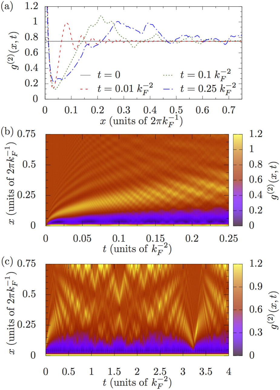
We now consider the evolution of the full nonlocal second-order correlation $g^{(2)}(x,t)$. In Fig. 9 we plot the behaviour of this quantity for an interaction quench from zero to $\gamma=-40$ for $N=4$ particles. Figure 9(a) shows $g^{(2)}(x,t)$ at four representative times $t$. Initially, $g^{(2)}(x,0)=1-1/N$ (horizontal line). At $t=0.01k_{F}^{-2}$ (red dashed line), the local value is already greatly enhanced, $g^{(2)}(0,t=0.01k_{F}^{-2})\simeq 3.5$, cf. Fig. 5(a). [The scale of the $y$ axis is chosen so that the long-range features of $g^{(2)}(x)$ are visible, and the large values for $x\lesssim 0.02\times(2\pi k_{F}^{-1})$ are therefore cut off.] In addition to the central peak, at separations $x\simeq 0.1\times(2\pi k_{F}^{-1})$ a secondary peak emerges, while at larger distances $g^{(2)}(x)$ exhibits a decaying oscillatory structure. As time progresses, this secondary peak propagates away from the origin and broadens as can be seen at, e.g. $t=0.1k_{F}^{-2}$ (green dotted line) and $t=0.25k_{F}^{-2}$ (blue dot-dashed line).

The build-up of this secondary correlation peak and its propagation through the system can be more clearly seen in Fig. 9(b), where we plot the time-evolution of $g^{(2)}(x,t)$ up to $t=0.25k_{F}^{-2}$. The propagation of this peak is consistent with $x(t)\propto t^{1/2}$, which was also observed for quenches from the same initial state to strongly repulsive interactions [32, 29]. (Note that the color scale is chosen so that the long-range behaviour is visible, and the local second-order correlation is again not resolved.) Figure 9(c) shows $g^{(2)}(x,t)$ for longer times up to $t=4\,k_{F}^{-2}$. The overall structure on this longer time scale is more complicated, with several soliton-like correlation dips propagating through the system [32] and a partial revival of $g^{(2)}(x,t=0)$ at $t\simeq 3.2k_{F}^{-2}$ [cf. Figs. 7(c) and 8(b)]. Besides the largely increased value at small distances, the behaviour of $g^{(2)}(x,t)$ is strikingly similar to the results obtained in Ref. [32] for quenches from the same noninteracting ground state to repulsive final interaction strengths.

In summary, quenches from the ideal-gas ground state to attractive values of $\gamma$ result in the occupation of energy eigenstates containing bound states in addition to the gas-like scattering states of the attractively interacting model, which are analogous to the eigenstates of the repulsively interacting Lieb–Liniger gas. As the magnitude $|\gamma|$ of the final interaction strength is increased, the postquench occupations of the gas-like excited states approach those of their counterparts following a quench to the corresponding repulsive interaction strength, and the occupations of bound states eventually decrease. However, these bound states significantly influence the dynamics of postquench correlation functions for all final interaction strengths we have considered, causing large oscillations in local correlations and in the occupation of the zero-momentum mode. For large attractive values of $\gamma$, bound states are highly localized and thus influence the second-order correlation function only at small separations, whereas at larger separations this function exhibits postquench dynamics similar to those observed following quenches to repulsive interactions [32].

In Fig. 10(a), we plot the enhancement of the diagonal-ensemble value $g^{(2)}_{\mathrm{DE}}(0)$ of the local second-order correlation over the initial noninteracting value $g^{(2)}_{\gamma=0}(0)$ of this function following an interaction quench from zero to $\gamma$ for particle numbers $N=2$, $3$, and $4$. For all particle numbers $N$ considered, as $|\gamma|$ is increased from the ideal-gas limit, $g^{(2)}_{\mathrm{DE}}(0)$ initially increases rapidly before reaching a local maximum, which occurs at smaller values of $|\gamma|$ for larger particle numbers $N$. For $N=4$ particles (solid blue line) this local maximum in $g^{(2)}_{\mathrm{DE}}(0)$ occurs at $\gamma=-1$ and coincides with the crossing of the population of the three-particle bound state $\{n_{j}\}=\{1,0\}$ and that of the ground state [see Fig. 3(a)]. The local minimum of $g^{(2)}_{\mathrm{DE}}(0)$ at $\gamma=-1.5$ coincides with the maximum population of this three-particle bound state, and as soon as the population of this state starts to decrease, $g^{(2)}_{\mathrm{DE}}(0)$ begins to increase monotonically with increasing $|\gamma|$.

For large attractive values of $\gamma$, the local second-order correlation tends to a constant value $g^{(2)}_{\mathrm{DE}}(0)/g^{(2)}_{\gamma=0}(0)\simeq 4$, which is much larger than the ideal gas and super-Tonks values [67]. The decrease of $g^{(2)}_{\mathrm{DE}}(0)$ with increasing particle number at fixed large $|\gamma|$ appears consistent with an approach toward the quench-action thermodynamic-limit strong-coupling value obtained to third order in $1/\gamma$ in Refs. [35, 36], indicated by the solid grey line, as $N\to\infty$.

Using the quench-action approach [71] in the thermodynamic limit, Refs. [35, 36] found that $g^{(2)}_{\mathrm{DE}}(0)=2$ for $\gamma\rightarrow 0^{-}$. Our methodology does not recover this result for small values of $|\gamma|$, as our small system sizes lead to a finite-size gap for excitations and therefore the energy added by the quench is small in this case. Additionally, eigenstates with more than four bound particles are trivially absent in our calculations, whereas for small postquench values of $|\gamma|$ they contribute significantly in the analysis of Refs. [35, 36]. For larger values of $|\gamma|$, however, states with more than two bound particles are strongly suppressed and we expect our results to be less influenced by finite-size effects [33].

In Fig. 10(b), we plot the enhancement of the diagonal-ensemble value of the local third-order correlation $g^{(3)}_{\mathrm{DE}}(0)$ over its noninteracting initial value following an interaction quench from zero to $\gamma$ for particle numbers $N=3$ and $4$. The qualitative behaviour is similar to that of $g^{(2)}_{\mathrm{DE}}(0)$. For strong interactions, $g^{(3)}_{\mathrm{DE}}(0)$ also tends to a constant value that is much larger than the initial value. Whether this result persists for larger atom numbers is an important open question, given that large values of $g^{(3)}(0)$ lead to strong recombination losses in experiments with ultracold gases [93, 94].

References

- [1] I. Bloch, J. Dalibard and W. Zwerger, Many-body physics with ultracold gases, Rev. Mod. Phys. 80, 885 (2008), 10.1103/RevModPhys.80.885.
- [2] T. Kinoshita, T. Wenger and D. S. Weiss, Local Pair Correlations in One-Dimensional Bose Gases, Phys. Rev. Lett. 95, 190406 (2005), 10.1103/PhysRevLett.95.190406.
- [3] T. Kinoshita, T. Wenger and D. S. Weiss, A quantum Newton’s cradle, Nature 440, 900 (2006), 10.1038/nature04693.
- [4] S. Hofferberth, I. Lesanovsky, B. Fischer, T. Schumm and J. Schmiedmayer, Non-equilibrium coherence dynamics in one-dimensional Bose gases, Nature 449, 324 (2007), 10.1038/nature06149.
- [5] M. Gring, M. Kuhnert, T. Langen, T. Kitagawa, B. Rauer, M. Schreitl, I. Mazets, D. Adu Smith, E. Demler and J. Schmiedmayer, Relaxation and Prethermalization in an Isolated Quantum System, Science 337, 1318 (2012), 10.1126/science.1224953.
- [6] T. Langen, R. Geiger, M. Kuhnert, B. Rauer and J. Schmiedmayer, Local emergence of thermal correlations in an isolated quantum many-body system, Nat. Phys. 9, 640 (2013), 10.1038/nphys2739.
- [7] E. Haller, M. Gustavsson, M. J. Mark, J. G. Danzl, R. Hart, G. Pupillo and H.-C. Nägerl, Realization of an Excited, Strongly Correlated Quantum Gas Phase, Science 325, 1224 (2009), 10.1126/science.1175850.
- [8] N. Fabbri, M. Panfil, D. Clément, L. Fallani, M. Inguscio, C. Fort and J.-S. Caux, Dynamical structure factor of one-dimensional Bose gases: Experimental signatures of beyond-Luttinger-liquid physics, Phys. Rev. A 91, 043617 (2015), 10.1103/PhysRevA.91.043617.
- [9] V. Guarrera, D. Muth, R. Labouvie, A. Vogler, G. Barontini, M. Fleischhauer and H. Ott, Spatiotemporal fermionization of strongly interacting one-dimensional bosons, Phys. Rev. A 86, 021601 (2012), 10.1103/PhysRevA.86.021601.
- [10] A. Vogler, R. Labouvie, F. Stubenrauch, G. Barontini, V. Guarrera and H. Ott, Thermodynamics of strongly correlated one-dimensional Bose gases, Phys. Rev. A 88, 031603 (2013), 10.1103/PhysRevA.88.031603.
- [11] D. Clément, N. Fabbri, L. Fallani, C. Fort and M. Inguscio, Exploring Correlated 1D Bose Gases from the Superfluid to the Mott-Insulator State by Inelastic Light Scattering, Phys. Rev. Lett. 102, 155301 (2009), 10.1103/PhysRevLett.102.155301.
- [12] B. Paredes, A. Widera, V. Murg, O. Mandel, S. Fölling, I. Cirac, G. V. Shlyapnikov, T. W. Hänsch and I. Bloch, Tonks-Girardeau gas of ultracold atoms in an optical lattice, Nature 429, 277 (2004), 10.1038/nature02530.
- [13] A. H. van Amerongen, J. J. P. van Es, P. Wicke, K. V. Kheruntsyan and N. J. van Druten, Yang-Yang Thermodynamics on an Atom Chip, Phys. Rev. Lett. 100, 090402 (2008), 10.1103/PhysRevLett.100.090402.
- [14] J. Armijo, T. Jacqmin, K. V. Kheruntsyan and I. Bouchoule, Probing Three-Body Correlations in a Quantum Gas Using the Measurement of the Third Moment of Density Fluctuations, Phys. Rev. Lett. 105, 230402 (2010), 10.1103/PhysRevLett.105.230402.
- [15] J. Armijo, T. Jacqmin, K. Kheruntsyan and I. Bouchoule, Mapping out the quasicondensate transition through the dimensional crossover from one to three dimensions, Phys. Rev. A 83, 021605 (2011), 10.1103/PhysRevA.83.021605.
- [16] T. Jacqmin, J. Armijo, T. Berrada, K. V. Kheruntsyan and I. Bouchoule, Sub-Poissonian Fluctuations in a 1D Bose Gas: From the Quantum Quasicondensate to the Strongly Interacting Regime, Phys. Rev. Lett. 106, 230405 (2011), 10.1103/PhysRevLett.106.230405.
- [17] F. Meinert, M. Panfil, M. J. Mark, K. Lauber, J.-S. Caux and H.-C. Nägerl, Probing the Excitations of a Lieb-Liniger Gas from Weak to Strong Coupling, Phys. Rev. Lett. 115, 085301 (2015), 10.1103/PhysRevLett.115.085301.
- [18] E. H. Lieb and W. Liniger, Exact Analysis of an Interacting Bose Gas. I. The General Solution and the Ground State, Phys. Rev. 130, 1605 (1963), 10.1103/PhysRev.130.1605.
- [19] E. H. Lieb, Exact Analysis of an Interacting Bose Gas. II. The Excitation Spectrum, Phys. Rev. 130, 1616 (1963), 10.1103/PhysRev.130.1616.
- [20] M. Olshanii, Atomic Scattering in the Presence of an External Confinement and a Gas of Impenetrable Bosons, Phys. Rev. Lett. 81, 938 (1998), 10.1103/PhysRevLett.81.938.
- [21] C. N. Yang and C. P. Yang, Thermodynamics of a One-Dimensional System of Bosons with Repulsive Delta-Function Interaction, J. Math. Phys. 10, 1115 (1969), 10.1063/1.1664947.
- [22] V. E. Korepin, N. M. Bogoliubov and A. G. Izergin, Quantum Inverse Scattering Method and Correlation Functions, Cambridge University Press, Cambridge, UK (1993).
- [23] M. Takahashi, Thermodynamics of One-Dimensional Solvable Models, Cambridge University Press, Cambridge, UK (1999).
- [24] M. A. Cazalilla, R. Citro, T. Giamarchi, E. Orignac and M. Rigol, One dimensional bosons: From condensed matter systems to ultracold gases, Rev. Mod. Phys. 83, 1405 (2011), 10.1103/RevModPhys.83.1405.
- [25] V. Gritsev, T. Rostunov and E. Demler, Exact methods in the analysis of the non-equilibrium dynamics of integrable models: application to the study of correlation functions for non-equilibrium 1D Bose gas, J. Stat. Mech. 2010, P05012 (2010), 10.1088/1742-5468/2010/05/P05012.
- [26] M. Kormos, A. Shashi, Y.-Z. Chou, J.-S. Caux and A. Imambekov, Interaction quenches in the one-dimensional Bose gas, Phys. Rev. B 88, 205131 (2013), 10.1103/PhysRevB.88.205131.
- [27] S. Sotiriadis and P. Calabrese, Validity of the GGE for quantum quenches from interacting to noninteracting models, J. Stat. Mech. 2014, P07024 (2014), 10.1088/1742-5468/2014/07/P07024.
- [28] P. Calabrese and P. Le Doussal, Interaction quench in a Lieb–Liniger model and the KPZ equation with flat initial conditions, J. Stat. Mech. 2014, P05004 (2014), 10.1088/1742-5468/2014/05/P05004.
- [29] M. Kormos, M. Collura and P. Calabrese, Analytic results for a quantum quench from free to hard-core one-dimensional bosons, Phys. Rev. A 89, 013609 (2014), 10.1103/PhysRevA.89.013609.
- [30] M. Collura, M. Kormos and P. Calabrese, Stationary entanglement entropies following an interaction quench in 1D Bose gas, J. Stat. Mech. 2014, P01009 (2014), 10.1088/1742-5468/2014/01/P01009.
- [31] J. De Nardis, B. Wouters, M. Brockmann and J.-S. Caux, Solution for an interaction quench in the Lieb-Liniger Bose gas, Phys. Rev. A 89, 033601 (2014), 10.1103/PhysRevA.89.033601.
- [32] J. C. Zill, T. M. Wright, K. V. Kheruntsyan, T. Gasenzer and M. J. Davis, Relaxation dynamics of the Lieb-Liniger gas following an interaction quench: A coordinate Bethe-ansatz analysis, Phys. Rev. A 91, 023611 (2015), 10.1103/PhysRevA.91.023611.
- [33] J. C. Zill, T. M. Wright, K. V. Kheruntsyan, T. Gasenzer and M. J. Davis, A coordinate Bethe ansatz approach to the calculation of equilibrium and nonequilibrium correlations of the one-dimensional Bose gas, New J. Phys. 18, 045010 (2016), 10.1088/1367-2630/18/4/045010.
- [34] G. Carleo, L. Cevolani, L. Sanchez-Palencia and M. Holzmann, Unitary Dynamics of Strongly Interacting Bose Gases with the Time-Dependent Variational Monte Carlo Method in Continuous Space, Phys. Rev. X 7, 031026 (2017), 10.1103/PhysRevX.7.031026.
- [35] L. Piroli, P. Calabrese and F. H. L. Essler, Multiparticle Bound-State Formation following a Quantum Quench to the One-Dimensional Bose Gas with Attractive Interactions, Phys. Rev. Lett. 116, 070408 (2016), 10.1103/PhysRevLett.116.070408.
- [36] L. Piroli, P. Calabrese and F. H. L. Essler, Quantum quenches to the attractive one-dimensional Bose gas: exact results, SciPost Phys. 1, 001 (2016), 10.21468/SciPostPhys.1.1.001.
- [37] J. B. McGuire, Study of Exactly Soluble One-Dimensional N-Body Problems, J. Math. Phys. 5(5), 622 (1964), 10.1063/1.1704156.
- [38] K. Sakmann, A. I. Streltsov, O. E. Alon and L. S. Cederbaum, Exact ground state of finite Bose-Einstein condensates on a ring, Phys. Rev. A 72, 033613 (2005), 10.1103/PhysRevA.72.033613.
- [39] A. G. Sykes, P. D. Drummond and M. J. Davis, Excitation spectrum of bosons in a finite one-dimensional circular waveguide via the Bethe ansatz, Phys. Rev. A 76, 063620 (2007), 10.1103/PhysRevA.76.063620.
- [40] F. Calogero and A. Degasperis, Comparison between the exact and Hartree solutions of a one-dimensional many-body problem, Phys. Rev. A 11, 265 (1975), 10.1103/PhysRevA.11.265.
- [41] L. Piroli and P. Calabrese, Local correlations in the attractive one-dimensional Bose gas: From Bethe ansatz to the Gross-Pitaevskii equation, Phys. Rev. A 94, 053620 (2016), 10.1103/PhysRevA.94.053620.
- [42] P. Calabrese and J.-S. Caux, Correlation Functions of the One-Dimensional Attractive Bose Gas, Phys. Rev. Lett. 98, 150403 (2007), 10.1103/PhysRevLett.98.150403.
- [43] P. Calabrese and J.-S. Caux, Dynamics of the attractive 1D Bose gas: analytical treatment from integrability, J. Stat. Mech. 2007, P08032 (2007), 10.1088/1742-5468/2007/08/P08032.
- [44] R. Kanamoto, H. Saito and M. Ueda, Quantum phase transition in one-dimensional Bose-Einstein condensates with attractive interactions, Phys. Rev. A 67, 013608 (2003), 10.1103/PhysRevA.67.013608.
- [45] G. M. Kavoulakis, Bose-Einstein condensates with attractive interactions on a ring, Phys. Rev. A 67, 011601 (2003), 10.1103/PhysRevA.67.011601.
- [46] D. Flassig, A. Pritzel and N. Wintergerst, Black holes and quantumness on macroscopic scales, Phys. Rev. D 87, 084007 (2013), 10.1103/PhysRevD.87.084007.
- [47] D. Flassig, A. Franca and A. Pritzel, Large- ground state of the Lieb-Liniger model and Yang-Mills theory on a two-sphere, Phys. Rev. A 93, 013627 (2016), 10.1103/PhysRevA.93.013627.
- [48] R. Kanamoto, H. Saito and M. Ueda, Symmetry Breaking and Enhanced Condensate Fraction in a Matter-Wave Bright Soliton, Phys. Rev. Lett. 94, 090404 (2005), 10.1103/PhysRevLett.94.090404.
- [49] R. Kanamoto, H. Saito and M. Ueda, Critical fluctuations in a soliton formation of attractive Bose-Einstein condensates, Phys. Rev. A 73, 033611 (2006), 10.1103/PhysRevA.73.033611.
- [50] Y. Lai and H. A. Haus, Quantum theory of solitons in optical fibers. II. Exact solution, Phys. Rev. A 40, 854 (1989), 10.1103/PhysRevA.40.854.
- [51] I. E. Mazets and G. Kurizki, How different are multiatom quantum solitons from mean-field solitons?, Europhys. Lett. 76, 196 (2006), 10.1209/epl/i2006-10260-0.
- [52] A. Ayet and J. Brand, The single-particle density matrix of a quantum bright soliton from the coordinate Bethe ansatz, J. Stat. Mech. 2017, 023103 (2017), 10.1088/1742-5468/aa58ac.
- [53] L. Khaykovich, F. Schreck, G. Ferrari, T. Bourdel, J. Cubizolles, L. D. Carr, Y. Castin and C. Salomon, Formation of a Matter-Wave Bright Soliton, Science 296, 1290 (2002), 10.1126/science.1071021.
- [54] K. E. Strecker, G. B. Partridge, A. G. Truscott and R. G. Hulet, Formation and propagation of matter-wave soliton trains, Nature 417, 150 (2002), 10.1038/nature747.
- [55] S. L. Cornish, S. T. Thompson and C. E. Wieman, Formation of Bright Matter-Wave Solitons during the Collapse of Attractive Bose-Einstein Condensates, Phys. Rev. Lett. 96, 170401 (2006), 10.1103/PhysRevLett.96.170401.
- [56] A. L. Marchant, T. P. Billam, T. P. Wiles, M. M. H. Yu, S. A. Gardiner and S. L. Cornish, Controlled formation and reflection of a bright solitary matter-wave, Nat. Commun. 4, 1865 (2013), 10.1038/ncomms2893.
- [57] J. H. V. Nguyen, P. Dyke, D. Luo, B. A. Malomed and R. G. Hulet, Collisions of matter-wave solitons, Nat. Phys. 10, 918 (2014), 10.1038/nphys3135.
- [58] P. Medley, M. A. Minar, N. C. Cizek, D. Berryrieser and M. A. Kasevich, Evaporative Production of Bright Atomic Solitons, Phys. Rev. Lett. 112, 060401 (2014), 10.1103/PhysRevLett.112.060401.
- [59] G. D. McDonald, C. C. N. Kuhn, K. S. Hardman, S. Bennetts, P. J. Everitt, P. A. Altin, J. E. Debs, J. D. Close and N. P. Robins, Bright Solitonic Matter-Wave Interferometer, Phys. Rev. Lett. 113, 013002 (2014), 10.1103/PhysRevLett.113.013002.
- [60] G. E. Astrakharchik, D. Blume, S. Giorgini and B. E. Granger, Quasi-One-Dimensional Bose Gases with a Large Scattering Length, Phys. Rev. Lett. 92, 030402 (2004), 10.1103/PhysRevLett.92.030402.
- [61] G. E. Astrakharchik, J. Boronat, J. Casulleras and S. Giorgini, Beyond the Tonks-Girardeau Gas: Strongly Correlated Regime in Quasi-One-Dimensional Bose Gases, Phys. Rev. Lett. 95, 190407 (2005), 10.1103/PhysRevLett.95.190407.
- [62] M. T. Batchelor, M. Bortz, X. W. Guan and N. Oelkers, Evidence for the super Tonks–Girardeau gas, J. Stat. Mech. 2005, L10001 (2005), 10.1088/1742-5468/2005/10/L10001.
- [63] S. Chen, L. Guan, X. Yin, Y. Hao and X.-W. Guan, Transition from a Tonks-Girardeau gas to a super-Tonks-Girardeau gas as an exact many-body dynamics problem, Phys. Rev. A 81, 031609 (2010), 10.1103/PhysRevA.81.031609.
- [64] M. D. Girardeau and G. E. Astrakharchik, Wave functions of the super-Tonks-Girardeau gas and the trapped one-dimensional hard-sphere Bose gas, Phys. Rev. A 81, 061601(R) (2010), 10.1103/PhysRevA.81.061601.
- [65] M. Panfil, J. De Nardis and J.-S. Caux, Metastable Criticality and the Super Tonks-Girardeau Gas, Phys. Rev. Lett. 110, 125302 (2013), 10.1103/PhysRevLett.110.125302.
- [66] D. Muth and M. Fleischhauer, Dynamics of Pair Correlations in the Attractive Lieb-Liniger Gas, Phys. Rev. Lett. 105, 150403 (2010), 10.1103/PhysRevLett.105.150403.
- [67] M. Kormos, G. Mussardo and A. Trombettoni, Local correlations in the super-Tonks-Girardeau gas, Phys. Rev. A 83, 013617 (2011), 10.1103/PhysRevA.83.013617.
- [68] D. Iyer and N. Andrei, Quench Dynamics of the Interacting Bose Gas in One Dimension, Phys. Rev. Lett. 109, 115304 (2012), 10.1103/PhysRevLett.109.115304.
- [69] D. Iyer, H. Guan and N. Andrei, Exact formalism for the quench dynamics of integrable models, Phys. Rev. A 87, 053628 (2013), 10.1103/PhysRevA.87.053628.
- [70] V. I. Yudson, Dynamics of the integrable one-dimensional system “photons + two-level atoms”, Phys. Lett. A 129, 17 (1988), 10.1016/0375-9601(88)90465-3.
- [71] J.-S. Caux and F. H. L. Essler, Time Evolution of Local Observables After Quenching to an Integrable Model, Phys. Rev. Lett. 110, 257203 (2013), 10.1103/PhysRevLett.110.257203.
- [72] J.-S. Caux, The Quench Action, J. Stat. Mech. 2016, 064006 (2016), 10.1088/1742-5468/2016/06/064006.
- [73] M. Rigol, V. Dunjko and M. Olshanii, Thermalization and its mechanism for generic isolated quantum systems, Nature 452, 854 (2008), 10.1038/nature06838.
- [74] H. B. Thacker, Exact integrability in quantum field theory and statistical systems, Rev. Mod. Phys. 53, 253 (1981), 10.1103/RevModPhys.53.253.
- [75] L. D. Carr, C. W. Clark and W. P. Reinhardt, Stationary solutions of the one-dimensional nonlinear Schrödinger equation. II. Case of attractive nonlinearity, Phys. Rev. A 62, 063611 (2000), 10.1103/PhysRevA.62.063611.
- [76] A. Montina and F. T. Arecchi, Many-body ground-state properties of an attractive Bose-Einstein condensate in a one-dimensional ring, Phys. Rev. A 71, 063615 (2005), 10.1103/PhysRevA.71.063615.
- [77] N. Oelkers and J. Links, Ground-state properties of the attractive one-dimensional Bose-Hubbard model, Phys. Rev. B 75, 115119 (2007), 10.1103/PhysRevB.75.115119.
- [78] L. Salasnich, Beyond mean-field theory for attractive bosons under transverse harmonic confinement, J. Phys. B 39, 1743 (2006), 10.1088/0953-4075/39/7/016.
- [79] Y. Castin, Bose-Einstein Condensates in Atomic Gases: Simple Theoretical Results, In R. Kaiser, C. Westbrook and F. David, eds., Coherent atomic matter waves, vol. 72 of Les Houches - Ecole d’Ete de Physique Theorique, pp. 1–136. Springer-Verlag, Berlin, 10.1007/3-540-45338-5_1 (2001).
- [80] Y. Castin and C. Herzog, Bose–Einstein condensates in symmetry breaking states, C. R. Acad. Sci., Ser. IV: Phys., Astrophys. 2, 419 (2009), 10.1016/S1296-2147(01)01183-0.
- [81] Y. Hao, Y. Zhang, J. Q. Liang and S. Chen, Ground-state properties of one-dimensional ultracold Bose gases in a hard-wall trap, Phys. Rev. A 73, 063617 (2006), 10.1103/PhysRevA.73.063617.
- [82] R. Paškauskas and L. You, Quantum correlations in two-boson wave functions, Phys. Rev. A 64, 042310 (2001), 10.1103/PhysRevA.64.042310.
- [83] M. Olshanii and V. Dunjko, Short-Distance Correlation Properties of the Lieb-Liniger System and Momentum Distributions of Trapped One-Dimensional Atomic Gases, Phys. Rev. Lett. 91, 090401 (2003), 10.1103/PhysRevLett.91.090401.
- [84] S. Tan, Energetics of a strongly correlated Fermi gas, Ann. Phys. 323, 2952 (2008), 10.1016/j.aop.2008.03.004.
- [85] M. Barth and W. Zwerger, Tan relations in one dimension, Ann. Phys. 326, 2544 (2011), 10.1016/j.aop.2011.05.010.
- [86] L. Pitaevskii and S. Stringari, Bose-Einstein Condensation, Oxford University Press, Oxford, UK (2003).
- [87] G. E. Astrakharchik and S. Giorgini, Correlation functions and momentum distribution of one-dimensional Bose systems, Phys. Rev. A 68, 031602 (2003), 10.1103/PhysRevA.68.031602.
- [88] J.-S. Caux, P. Calabrese and N. A. Slavnov, One-particle dynamical correlations in the one-dimensional Bose gas, J. Stat. Mech. 2007(01), P01008 (2007).
- [89] V. V. Cheianov, H. Smith and M. B. Zvonarev, Exact results for three-body correlations in a degenerate one-dimensional Bose gas, Phys. Rev. A 73, 051604 (2006), 10.1103/PhysRevA.73.051604.
- [90] D. M. Gangardt and G. V. Shlyapnikov, Stability and Phase Coherence of Trapped 1D Bose Gases, Phys. Rev. Lett. 90, 010401 (2003), 10.1103/PhysRevLett.90.010401.
- [91] P. J. Forrester, N. E. Frankel and M. I. Makin, Analytic solutions of the one-dimensional finite-coupling delta-function Bose gas, Phys. Rev. A 74, 043614 (2006), 10.1103/PhysRevA.74.043614.
- [92] D. Muth, B. Schmidt and M. Fleischhauer, Fermionization dynamics of a strongly interacting one-dimensional Bose gas after an interaction quench, New J. Phys. 12, 083065 (2010), 10.1088/1367-2630/12/8/083065.
- [93] E. Haller, M. Rabie, M. J. Mark, J. G. Danzl, R. Hart, K. Lauber, G. Pupillo and H.-C. Nägerl, Three-Body Correlation Functions and Recombination Rates for Bosons in Three Dimensions and One Dimension, Phys. Rev. Lett. 107, 230404 (2011), 10.1103/PhysRevLett.107.230404.
- [94] C. Chin, R. Grimm, P. Julienne and E. Tiesinga, Feshbach resonances in ultracold gases, Rev. Mod. Phys. 82, 1225 (2010), 10.1103/RevModPhys.82.1225.
- [95] J. Berges and T. Gasenzer, Quantum versus classical statistical dynamics of an ultracold Bose gas, Phys. Rev. A 76, 033604 (2007), 10.1103/PhysRevA.76.033604.
- [96] M. Girardeau, Relationship between Systems of Impenetrable Bosons and Fermions in One Dimension, J. Math. Phys. 1, 516 (1960), 10.1063/1.1703687.
- [97] E. Kaminishi, J. Sato and T. Deguchi, Recurrence time in the quantum dynamics of the 1D Bose gas, J. Phys. Soc. Jpn. 84, 064002 (2015), 10.7566/JPSJ.84.064002.
- [98] A. Polkovnikov, K. Sengupta, A. Silva and M. Vengalattore, Colloquium: Nonequilibrium dynamics of closed interacting quantum systems, Rev. Mod. Phys. 83, 863 (2011), 10.1103/RevModPhys.83.863.