Road to micron resolution with a color X-ray camera – polycapillary optics characterization
Stanisław H. Nowak,∗ab Marko Petric,cd Josef Buchriegler,d Aniouar Bjeoumikhov,af Zemfira Bjeoumikhov,a Johannes von Borany,d Frans Munnik,d Martin Radtke,g Axel D. Renno,h Uwe Reinholz,g Oliver Scharf,a Joachim Tilgner,a and Reiner Wedelli
In a color X-ray camera spatial resolution is achieved by means of a polycapillary optic conducting X-ray photons from small regions on a sample to distinct energy dispersive pixels on a CCD matrix. At present, the resolution limit of color X-ray camera systems can go down to several microns and is mainly restricted by pixel dimensions. The recent development of an efficient subpixel resolution algorithm allows a release from pixel size, limiting the resolution only to the quality of the optics. In this work polycapillary properties that influence the spatial resolution are systematized and assessed both theoretically and experimentally. It is demonstrated that with the current technological level reaching one micron resolution is challenging, but possible.
1 Introduction
In the last decades X-ray fluorescence (XRF) underwent an evolution from broad area element analysis towards spatially resolved elemental imaging 1. A conventional approach to spatially resolved XRF employs a focused X-ray beam to map the fluorescence of a given sample region 2. Each mapping position is reached using a fine mechanical -stage. XRF spectra are achieved for each scanning position by means of energy resolved detectors.
In the last years a cross over from compact 1-D detectors to spatially resolving detectors was obtained with the use of polycapillary optics and charge coupled devices (CCD) 3, 4, 5, 6. However, most of these detection systems can only measure spatial information at a pixel size and without energy resolution.7, 4, 8, 9
The recent development of SLcam® 10, 11, 12 filled that gap bringing a high quantum efficiency and throughput color X-ray camera system that combines a spatially and spectrally resolving pn-junction Charged-Coupled Device (pnCCD) from PNSensor in Munich13 with polycapillary optics 14 from IfG – Institute for Scientific Instruments GmbH in Berlin.
The pnCCD detector is designed for ultrafast readout allowing detection of single photons with both spatial and energy resolution. Single photon counting mode is achievable even at relatively high photon count rates as available at synchrotron or PIXE endstations.15
A standalone pnCCD is used for spatially resolved X-ray transmission16, diffraction17 or scattering measurements18. However, in order to achieve an image of X-ray fluorescence, X-ray photons should be explicitly guided from small regions on a sample to corresponding pixels on a detector. For this a polycapillary optic is used that can be regarded as a bunch of independent X-ray channels bringing the photons from the source to a proper section of a CCD, similarly to the way a fiber optic guides light. The color X-ray camera uses conical and parallel polycapillary structures. Conical polycapillary optics can be used for magnification of the image. Straight structures are used to obtain a 1:1 image on the detector.
The lateral resolution of a color X-ray camera is limited by both the pixel dimension and entry diameter of a single capillary. Currently used SLcam® optics are optimized for pnCCD pixel dimension of .12, 11 The capillary exit diameter is adapted in such a way, that a spot size from an individual channel on the detector is approximately equal to the pixel size. Keeping the pixel size fixed, the spatial resolution can be seriously improved by the use of conically shaped magnifying optics. In this case the signal reaching a single pixel on the detector originates from a much smaller area on a sample. The drawback is a limited filed of view.
With the use of subpixel algorithm the dominant role of the pixel size is released.19 This algorithm divides the signal assigned to each physical pixel over a number or virtual subpixels. Such an approach gives room for further downscaling of channels, and consequently, to improvement of the spatial resolution. In this paper the polycapillary physical parameters, including but not limited to channels’ diameter, are asses and the influence of these parameters on the imaging capabilities is investigated.
2 Spatial resolution
Spatial resolution is the ability of an imaging device to capture finely spaced details. Typically it is assessed as – the maximum frequency of bright-dark line pairs in a unit length that can be visibly resolved with a specified contrast level. Alternatively, resolution can be describe in a reciprocal manner as resolving power or resolution limit, i.e., the shortest distance of two objects at which a contrast above a specified limit can be maintained.
It should be noticed than the concept of resolution is associated with a certain ambiguity.20 First, the cut-of contrast level can be chosen in many, equally good manners. Second, in real measurements the contrast increases with the signal to noise ratio. The latter in turn is an increasing function of the image acquisition time and illumination, and can vary from one measurement to another.
2.1 Theoretical limits to resolution
There are some theoretical limits to spatial resolution. The Nyquist–Shannon sampling theorem 21 says that the highest possible frequency that can be correctly reproduced from a discrete sampled signal is half of the sampling rate. In other words, making samples over a certain distance only a signal comprising less than elements can be correctly distinguished. A higher number of elements will lead to signal aliasing resulting in distortions and artifacts. In the case of color X-ray camera that means that correct rendering of elements smaller than double the capillary channel size should not be possible.
Another concept that can be used to theoretically assess the spatial resolution is the response of an imaging system to a point source, the so-called Point Spread Function (PSF). If the shape of the PSF is known, then the resolution power can be calculated as – the smallest distance at which the signal from two point sources of equal intensity creates a valley (lowest value of signal) lower than the contrast limit. In particular for a system with a Gaussian type PSF, is always larger than the Full Width at Half Maximum (FWHM) – a sum of two Gaussian distributions that meet at their FWHM does not crate a valley.
Concluding, the spatial resolution is limited by the maximum of two - double the sampling distance , and the size of the Point Spread Function:
| (1) |
In the optimal case the sampling distance should be smaller than a half of . Such a spatial oversampling prevents creation of aliases and also increases the available contrast.
2.2 Contrast Transfer Function
Experimentally, the spatial resolution may be determined from the Contrast Transfer Function (CTF) that can be measured using standardized resolution test charts.22 Typical test structures consist of repeated bar patterns or concentric wedges. CTF gives the contrast between the test chart structure and the background as a function of structure dimensions or periodicity (i.e., lines per mm). The spatial resolution is a point at which the contrast drops below the chosen level. Proper measurement of CTF requires a long enough image acquisition time to ensure that the noise level is below the contrast cut-off value.
2.3 Sub-pixel resolution
Pixel resolution, understood as total number of pixels across the entire width and height of an image, inevitably limits the spatial resolution in a way predetermined by the Nyquist-Shannon theorem. The details smaller than twice the pixel size cannot be rendered correctly. In the case of color X-ray camera, however, the dominant role of pixel size can be released with the use of a subpixel resolution algorithm.19, 23, 24 The algorithm divides the signal assigned to each physical pixel over a number or virtual subpixels, increasing the pixel count and bypassing the Nyquist-Shannon theorem limitation.
Images with subpixel resolution are achievable due to the specific physics of the interaction of X-ray photons with a CCD’s Si layer. An X-ray photon that is absorbed in a fully depleted silicon layer generates a so-called electron cloud with a number of electrons proportional to the photon energy. Because the cloud has a nonzero area the generated electrons are deposited in several pixels closest to the photon hit location. With a correct reconstruction of the charge footprint the photon hit position can be estimated with a much higher precision than the pixel size. In the case of the SLcam® a pixel division up to 55 subpixels can be safely applied.19
2.4 Spatial resolution of SLcam®
The resolution limit of a color X-ray camera is restricted by the larger of two factors: – the width of the PSF of a polycapillary optic, or double the sampling distance. With the use of subpixel resolution the sampling distance can be practically identified with the capillary channel diameter .
The best performance is achieved, if the subpixel size is smaller than the half of the resolution limit of a polycapillary. In other words the subpixel dimension should be smaller than at least one of two factors: the channel diameter or half of .
3 Polycapillary optics


A polycapillary optic is a bundle of glass tubes with a typical diameter of several microns separated by thin walls. For the case of imaging it can be regarded as a bunch of independent X-ray channels gathering the photons from the X-ray source and bringing them to a section of the CCD. The operating principle of polycapillary optics is based on the effect of total external reflection. Below – the critical angle of total reflection, which depends mainly on the reflecting material and the X-ray photon energy, the reflection coefficient reaches values near to 100%. In addition, the low roughness of the reflective glass surface results in a low amount of diffuse scattered X-rays. As a result X-ray radiation is very effectively transported through an optic being reflected at the inner surface of the capillary channels. A schematic view of a politically optic is shown in Figure 1.
Thanks to the plasticity of glass, a polycapillary optic can be bent and shaped during the fabrication process. The polycapillary objectives are manufactured with either parallel and straight, or tapered channels. For the latter the entrance diameter is smaller than the exit .
Straight, parallel optics are ideal for one to one imaging. This specific capillary geometry results in a deep depth of sharpness, making it excellent to visualize uneven objects 25. Conically shaped polycapillaries are used for optical magnification. Magnification factors up to are attainable with the current fabrication technology.
In the SLcam® the optic housing and the camera head are connected via a fine screw thread to a thin Be entrance window of the camera, allowing rapid changing of the X-ray lenses. The pnCCD chip is located below that window. The optic housing leaves an additional space to prevent any damage of the fragile Be window. All together the optic-detector clearance is about .
3.1 Transmission, Acceptance, Sensitivity
The optical transmission of a polycapillary is strongly coupled to its open area ratio , i.e., the ratio of the polycapillary area that is not occupied by the glass to the total area. The maximum transmission of a parallel X-ray beam perfectly aligned to the polycapillary channels should not exceed . An exception to that is the hard X-ray regime in which glass becomes transparent, allowing an X-ray beam to penetrate the whole length of polycapillary facets.
It should be noticed that a polycapillary can only propagate photons entering within a certain acceptance cone. The acceptance cone is a result of X-ray reflections in the channels and, in case of a magnifying lens, also the conical shape of an optic. The half-angle of the acceptance cone, the so called acceptance angle , is roughly the sum of the critical angle for total reflection and half of the conical aperture of a channel :
| (2) |
There are opposing causes for deviations from that sum. First is that the probability of a photon transfer decreases with the number of bounces of the X-ray beam. In Figure 2 the transmission probabilities are presented as reflectivity curves for different numbers of reflections. For a large number of bounces the angular range for effective transmission is strongly reduced. A not negligible surface roughness and waviness of polycapillary channels further reduce the reflectivity in consecutive bounces. Second effect is related to possible spiral photon propagation in a polycapillary channel.26 This effect enlarges the acceptance cone and is most of all related to conical optics where the number of bounces is reduced. Another effect, related to conical polycapillaries, is the halo that occurs when X-rays penetrate the walls between channels and are totally reflected in a neighboring channel.27
Obviously, a nonzero acceptance angle leads to an increased number of photons transmitted by an optic. Accordingly, the parallel beam transmission is not a sufficient parameter to characterize the polycapillary’s ability to collect photons. In this regard a much better quantity is the optical sensitivity that can be defined as a rate of photons emitted from a point source that are first collected and then transmitted by an optic. In order to correctly evaluate , the transmission of the radiation of a point source is integrated over the complete solid angle and divided by 4 for normalization purpose:
| (3) |
where and are the angular directions of the emitted radiation. Accordingly, is the ratio between the number of photons transmitted trough the optic and the total number of photons emitted from a point source in the full solid angle.
3.2 Point Spread Function
The acceptance cone increases the photon collection efficiency, but also leads to a certain image blur. The point source signal arriving to a polycapillary is accepted in a spot of a diameter which can be calculated from the acceptance angle and the sample-optic distance :
| (4) |
Each irradiated capillary channel transfers the photons to its exit and creates a divergent beam reaching the detector. For a parallel 1:1 optic the divergent beam has the same shape as the acceptance cone. For the tapered, magnifying polycapillaries the half-angle of the divergence cone is always smaller than , but also bigger than half of the conical aperture of a channel:
| (5) |
The size of a single channel footprint on a detector is a function of: – capillary diameter at the exit (), – polycapillary divergence angle, and – the optic-detector clearance:
| (6) |
The PSF can be estimated as a convolution of a single channel footprint and a magnified acceptance spot. Supposing that both have a Gaussian shape, the FWHM of the resulting PSF equates to
| (7) |
where is multiplied by the optic magnification factor .
3.3 Resolving power
According to eq. (1) – the resolving power of a polycapillary optic can be estimated from and capillary diameter . Consequently, has its lower limit in or, following Nyquist-Shannon theorem, in :
| (8) | |||||
| (9) |
Having such an estimate the influence of each parameter can be evaluated.
For the case of nonzero acceptance () and divergence (), grows with the sample-optic () and optic-detector () distances. Typical values for and are at a level of several millimeters. As , and count in milliradians, the additional spreading is in micrometer range. It should be noted that in case of magnifying optics (), has a less significant influence on .
When and , or both and move toward , the lower limit on resolving power, calculated with (8), approaches the capillary channel diameter , i.e., the polycapillary sampling distance. In this case the resolution is determined by the Nyquist-Shannon theorem limitation (9).
Finally, decreases with photon energy. This is a consequence of the fact that both and scale with the total reflection angle, which itself is inversely proportional to energy:
| (10) |
4 Experimental
4.1 Characterization of polycapillaries
Parameters such as: magnification , channel entrance diameter , fractional open area , etc., affect the performance of an optic altering its angular acceptance , divergence , and optical sensitivity . In order to elucidate this influence, various polycapillaries, made of the same glass material, were investigated. Table 1 presents the comparison of physical parameters of the measured polycapillaries. In the experiments the parallel beam transmission , acceptance angle , and sensitivity were measured.
| Optic: | 1:1/60 | 1:1/24 | 1:1/20() | 1:1/7 | 8:1/2 |
| – magnification: | 1 | 1 | 1 | 1 | 8 |
| – entrance: | 60 | 24 | 20 | 7 | 2 |
| – exit: | 60 | 24 | 20 | 7 | 16 |
| – length: | 3 | 3 | 3 / 7 ∗ | 3 | 8 |
| – conical aperture: | |||||
| – field of view: | 1212 | 1212 | 1212 | 77 | 1.51.5 |
| – open area ratio: | 73 | 56 | 75 | 50 | 56 |
∗Polycapillaries 1:1/20(3) and 1:1/20(7) were produced in the same fabrication process and differ in length only.

The experimental setup (see Figure 3) comprised a micro-beam X-ray tube as an X-ray source. A pinhole was mounted at a large enough distance () to achieve an X-ray beam with a low divergence of around . The optics were installed on a - motorized stage allowing rotation in both directions perpendicular to the beam. The transmitted intensity was measured by a 1D silicon drift detector (Bruker AXS Xflash Detector 430). The 2D angular scans were performed with a step of giving the angular distribution maps of transmission.
Alternatively, polycapillary parameters were assessed with the use of SLcam® imaging. For that purpose an image of a distant () micro-beam X-ray tube was detected. In such an arrangement the polycapillary is accessed by X-rays at various incidence angles, generating an angular map in analogy to that obtained in a scan. Each pixel of an SLcam® map covers an angular range of , where is the pixel size.
The polycapillary optic characterization was performed in air; thus, the relevant data could only be obtained for X-ray energies above 6 keV – the low energy part of radiation was absorbed. In both setups beam intensity without a polycapillary optic was measured as a reference for transmission. The X-ray tube was to be operated at very low intensities to avoid the creation of pileups.
The maximum of the transmission map was identified as the transmission of a polycapillary; the optical sensitivity was obtained as the total sum of intensities multiplied by the angular step sizes and and divided by ,
| (11) | |||||
| (12) |
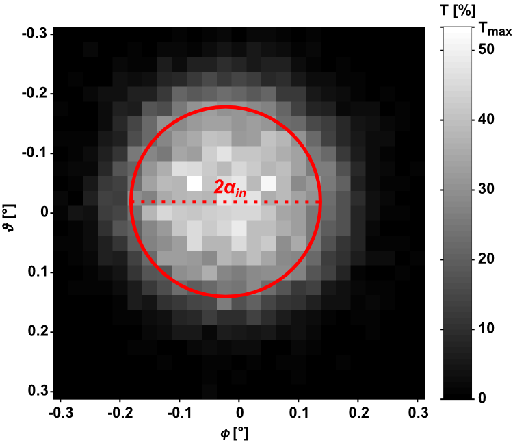
where is the value of a single element of the transmission map. The angular acceptance for a given energy range was calculated as the half width at half maximum of a 2D Gaussian fitted to the map. An exemplary distribution map of X-ray transmission is presented in Figure 4.
4.2 Assessment of SLcam® resolution
To evaluate the resolution of the SLcam® we used Sn Siemens star patterns fabricated at Fraunhofer IZM in Berlin. The Siemens star is deposited on a Si support and consists of concentric, evenly distributed Sn stripes and a little central alignment disc. A thin Cu layer was used to improve the adhesion of the Sn elements. The closer to the center of the structure, the Sn stripes are becoming thinner and the spacing between them narrower. At a certain point the dimensions are so little that the contrast between the structure and the background is below the predefined limit and stripes cannot be resolved. This is observed as a gray disk around the center of the Siemens star.

The spatial resolution can be estimated from the radius of the gray disk and the number of line pairs in a given central angle of the Siemens star (see Figure 5). The resolution can be given either as a maximal perceptible line frequency
| (13) |
or as resolution limit, i.e., the minimal width that is still distinguishable:
| (14) |
An accurate measure of the can be assessed from CTF. For each value of a radius a sinusoid is fitted to an arc spanned on the the Siemens Star. The value of CTF is obtained as the ratio of the sinusoid amplitude to the average intensity on the arc. is found as the largest radius for which CTF is below the predefined contrast level. In Figure 5 an example assessment of for contrast levels of 20% and 10% are shown.
SLcam® measurements were performed employing synchrotron radiation and proton beam excitation. The synchrotron light was provided by the BAMline at BESSY II.28 The proton beam was accessed at a newly developed High-Speed PIXE (HS-PIXE) beam line at Ion Beam Center at Helmholtz-Zentrum Dresden-Rossendorf (HZDR). 29
5 Results

5.1 Polycapillaries
In Figure 6 different optics are compared for their parallel beam transmission , angular acceptance angle , and optical sensitivity . The parameters are plotted as a function of photon energy between . For SLcam® measurements the energy range spans from .
The open area ratios () listed in Table 1, correspond quite well to the maximal values of the parallel beam transmission . The most significant discrepancy is seen for 1:1/20(3) optic. As an effect of its extensive use, this polycapillary has been stained with fingerprints and dust that attenuate the X-ray radiation. For some other optics (1:1/60 and 1:1/24) is slightly overestimated. This overestimation seems to be a result of a noise sensitive quantification procedure that selects the most intense pixel from a transmission map (see Section 4.1).
For most polycapillaries is rather stable, and this is what should be expected for parallel structures. 30 However, for some polycapillaries the transmission first rises and then drops with energy. This effect can be attributed to a deflection from parallel structure geometry and is normally observed for curved polycapillaries where X-ray radiation is always transmitted in a series of bounces. 31 The transmission drop in higher energies is mostly caused by the decrease of the total reflection angle. But, as was already presented in Figure 2, the increased number of bounces in the structure also decreases the transmission probability. This effect is even more pronounced for lower energies. Accordingly, for a magnifying optic the parallel beam propagates without bounces only in a limited number of channels; the others are approached at a certain angle. This is also the case for imperfect parallel optics for which the channels are slightly bended similarly as in a curved polycapillary.
Even though all the polycapillaries are made of the same glass material, the values of angular acceptance differ significantly from one objective to another. Nevertheless, for all the optics is inversely proportional to photon energy (10), and follows the trend of – critical angle for total reflection. Note also that, except for the 8:1/2 optic, the angular acceptance is always below . Optic 8:1/2 exhibits the largest angular acceptance. This is an effect of conical geometry, that, according to equation (2), systematically raises the acceptance by – the half of conical aperture of a polycapillary channel. For parallel optics a clear trend is that lower ratio results in a lower angular acceptance. For thin and long channels the number of bounces is much higher that for the wider and longer ones. This decreases the probability of a photon transmission. For example an X-ray beam entering the 1:1/7 optic at would be reflected on the inner wall of a channel over 200 times; for the case of 1:1/60 optic the beam would encounter less than 30 bounces.
The optical sensitivity does not follow the trend of the parallel beam transmission . is proportional rather to a product of and . As a result, for the optics with a relatively low transmission but high enough acceptance angle, can be still significant. For 1:1/60 optic an increase of can be observed for X-ray energies above . In this regime the optic becomes transparent to X-rays and photons begin to penetrate trough the facets not being absorbed.
Note that , similarly to , decreases with energy. Consequently, the best optic sensitivity is expected for soft X-rays.
5.2 Resolution
| measured | calc. | ||||||||||||
| Optic | [mm] | ROI | [m] | [m] | [m] | ||||||||
| 11 | 22 | 33 | 44 | 11 | 22 | 33 | 44 | ||||||
| : | 48 | 24 | 16 | 12 | 48 | 24 | 16 | 12 | : | ||||
| 1:1/20(3) | 10 | Sn L | 96.7 | 94.1 | 93.4 | 93.4 | 76.2 | 61.0 | 60.0 | 60.0 | — | ||
| Cu K | 73.8 | 67.3 | 66.9 | 66.6 | 62.1 | 53.3 | 51.3 | 49.7 | 48.9 | ||||
| 1:1/20(7)∗ | 7 | Sn L | 70.3 | 64.4 | 62.3 | 62.3 | 59.3 | 50.3 | 46.2 | 45.8 | — | ||
| Cu K | 63.1 | 53.1 | 53.4 | 53.1 | 51.4 | 44.5 | 44.1 | 44.5 | 42.5 | ||||
| 1:1/7 | 14 | Sn L | 78.0 | 68.6 | 67.0 | 67.0 | 63.0 | 53.2 | 52.3 | 52.6 | — | ||
| Cu K | 62.4 | 53.1 | 52.1 | 52.1 | 53.0 | 45.9 | 43.9 | 43.6 | 41.4 | ||||
| : | 6 | 3 | 2 | 1.5 | 6 | 3 | 2 | 1.5 | : | ||||
| 8:1/2 | 1 | Sn L | 8.0 | 7.0 | 7.0 | 6.6 | 6.6 | 5.6 | 5.6 | 5.6 | — | ||
| Cu K | 6.5 | 5.0 | 4.8 | 4.6 | 5.2 | 4.0 | 4.0 | 3.9 | 3.7 | ||||
| measured | calc. | ||||||||
| [LP/mm] | [LP/mm] | [LP/mm] | |||||||
| 11 | 22 | 33 | 44 | 11 | 22 | 33 | 44 | ||
| 10.4 | 20.8 | 31.2 | 41.7 | 10.4 | 20.8 | 31.2 | 41.7 | ||
| 5.2 | 5.3 | 5.4 | 5.4 | 6.6 | 8.2 | 8.3 | 8.3 | — | |
| 6.8 | 7.4 | 7.5 | 7.5 | 8.1 | 9.4 | 9.7 | 10.1 | 10.2 | |
| 7.1 | 7.8 | 8.0 | 8.0 | 8.4 | 9.9 | 10.8 | 10.9 | — | |
| 7.9 | 9.4 | 9.4 | 9.4 | 9.7 | 11.2 | 11.3 | 11.2 | 11.7 | |
| 6.4 | 7.3 | 7.5 | 7.5 | 7.9 | 9.4 | 9.6 | 9.5 | — | |
| 8.0 | 9.4 | 9.6 | 9.6 | 9.4 | 10.9 | 11.4 | 11.5 | 12.1 | |
| 83 | 167 | 250 | 333 | 83 | 167 | 250 | 333 | ||
| 62.2 | 71.1 | 71.6 | 76.1 | 75.6 | 88.5 | 88.5 | 89.1 | — | |
| 76.6 | 100 | 104 | 110 | 95.6 | 126 | 124 | 128.4 | 136 | |
∗ Measurements with 1:1/20(7) optic were performed at the HS-PIXE beam line at HZDR.

The resolution of the SLcam® was evaluated for different types of optics and for two energy regions: the Sn L line series from , and the Cu K line series from . The use of these two energy ranges was possible due to the specific structure of the Siemens star that employs a thin Cu layer to improve the adhesion of the Sn elements. The assessment of the resolution was performed for 1x1, 2x2, 3x3 and 4x4 subpixel divisions of acquired images. The cutoff contrast level was specified as 10% and 20%.
Table 2 lists the obtained measures of the resolution given as resolving power and as the line pairs frequency . For the Cu K line series these quantities are compared to theoretical values: the size of a point spread function , and the corresponding resolution limit . Theoretical values were calculated using equation (8) employing parameters from Table 1 and Figure 6 (for focusing 8:1/2 optic was measured to be ; for all the optics the distance to the detector is ). For comparison the table also gives the size of a single subpixel and the Nyquist-Shannon frequency for corresponding subpixel divisions.
In most cases a subpixel division gives already very good results. Further pixel division only slightly improves the resolution. The choice of the contrast level significantly affects the obtainable resolution. In all the cases the resolution limit going from to is improved by and closely approaches the theoretical limit of when subpixel resolution is applied. These results are illustrated in Figure 7.

A very important aspect when using polycapillary optics is the strong energy dependence of resolution. According to equation (8) the resolving power of a polycapillary should scale with the acceptance angle which is inversely proportional to energy. As a result the images are subject to chromatic aberration – a better resolving power is expected for higher X-ray energies. This trend was observed for all the polycapillaries – the resolution limits achieved for Cu K line series are always better then the ones obtained for Sn L lines.
The influence of the sample-optic distance on imaging is another effect that strongly influences the measurement. As stated in Section 3.3 the size of a point spread function is reduced when minimizing . As a result the resolving power is improved, but also the resolution variation with energy is decreased. This can be seen in Figure 8 where results obtained at various distances and for different energy regions are compared.
5.3 Real sample example

In order to present the color X-ray camera performance on a real sample a snail radula was measured with the 8:1/2 focusing optic using synchrotron light set to the energy of 10 keV. The false color image presented in Fig. 9 was obtained by superposing color maps corresponding to the intensity of scattered X-ray radiation and the characteristic fluorescence lines of Fe and Cu. The main image represents the whole available SLcam® chip area of pixels and was rendered in subpixel resolution. In the insets smaller details of the image are compared for standard and subpixel resolution.
As expected the subpixel resolution makes it possible to resolve small overlapping elements. With the optic used it was possible to resolve several micrometer spots at the energies of Fe K and Cu K lines (see inset a.).
In the presented image the scattered radiation follows the pattern of the Fe K image. As a result the chromatic aberration can be clearly seen – the lower energy image is more blurred and creates a border fringe around the higher energy image – this is illustrated in the inset b.
Finally, the polycapillary optic defects (see inset c.) can serve as a measure of the lowest resolution limit that could be obtained with the optic. The image of the optic’s defects does not result from the imaging object, instead it is created within a polycapillary. For that reason should be set to in order to evaluate its resolution with equation (8). The resulting resolving power limit is . And indeed, hexagonal lines of width comparable with the subpixel size of can be resolved.
6 Conclusions
The resolution of a polycapillary optic is a function of many factors. Some of them, like sample to optics distance, or the energy region used for imaging can be adapted on a regular basis depending on a running experiment. However, most of the resolution sensitive parameters are defined during the polycapillary fabrication process. This includes, but is not limited to, the channel diameter, the glass material used, and the magnification factor.
The most relevant parameter for resolution is the channel entrance diameter . The polycapillary resolving power given by the Nyquis-Schannon theorem is about . Besides, is also the ultimate limit for resolving power resulting from the size of the point spread function.
The image resolution can be considerably improved by reducing the sample-optic distance. Accordingly, the best resolution would be achieved if the sample was positioned directly on the lens. Such a setup could be realized, e.g., in reversed TXRF geometry where the polycapillary objective covered by a thin foil would serve as a reflector. Such a setup would prevent the detection of the primary beam radiation.
In practice such a radical shortening of the sample-optic distance would be effective only for the focusing optics. In case of parallel optics the spacing effect is less dramatic, due to a more significant influence of the optic-detector gap, and a distance is sufficient to obtain a maximum improvement of the resolution. In Table 3 the size of the PSF is compared for a sample-optic distance of and direct positioning on the objective. In case of a focusing optic the resolution limit can be decreased by a factor of 2; not much difference is encounter in case of parallel optics, however. Note that such a close sample installation brings the size of PSF below the resolution limit given by the Nyquist-Schannon theorem which is double the size of a capillary channel.
| Optic: | 1:1/20(3) | 1:1/7 | 8:1/2 |
|---|---|---|---|
| 1 | 35.8 | 21.3 | 4.3 |
| 0 | 35.7 | 21.1 | 2.7 |
The spatial resolution varies with X-ray energy following the change in critical angle of total reflection . As a consequence, the resolution is improved for higher energies. In addition to the energy dependence, the value of is strongly influenced by the properties of the reflecting material. The higher the optical density of the material, the lower is. Accordingly, the size of a PSF, and consequently the resolution limit, can be seriously reduced if a glass with a high Pb concentration is used. However, a decrease of entails a decrease of acceptance angle and, as a result, the polycapillary sensitivity would be reduced. Therefore the fabrication of polycapillary objectives needs to compromise the need for better resolution with good enough optics sensitivity.
In order to visualize the images with the resolution given by the polycapillary lens an appropriate pixel size is needed. In this respect a subpixel resolution algorithm is a very productive tool. However, the maximum number of subpixel divisions is restricted by the electronic properties of the detector (see Section 2.2). In addition the pixel division results in a lower number of counts in each virtual pixel; consequently, the available contrast is decreased.
Image resolution can be significantly improved when magnifying optics with a conical shape are employed. The conical optics, however, have high acceptance angles and can exhibit a halo.32
With all that said, arriving at a resolving power of is challenging and would require at most a entrance channel. Research on a further reduction of the capillary channel diameter and halo minimization are pursued. An objective with channel dimensions below can be expected in the near feature.
Authors Contribution
SHN, MP, AB, ZB, JT, OS, and RW designed and planned the polycapillary characterization experiment. AB and ZB provided the polycapillary optics. JT created motorization and acquisition software. SHN and MP performed the polycapillary characterization. MR and UR realized imaging at synchrotron radiation facility. SHN, JB, JvB, FM, ADR, and OS carried out PIXE measurements. SHN and OS provided the image rendering and analyzing software. SHN, MP, JB, and OS handled the data. SHN analyzed the data, carried out the calculations and wrote the manuscript. All the authors reviewed the manuscript.
Acknowledgments
We thank Björn Stelbrink and Andreas Wessel (Museum für Naturkunde Berlin) for providing the snail radula sample. This work has been supported by Marie Curie Actions - Initial Training Networks (ITN) as an Integrating Activity Supporting Postgraduate Research with Internships in Industry and Training Excellence (SPRITE) under EC contract no. 317169. SHN acknowledges financial support from the Swiss National Science Foundation (SNSF), Project no. 148569.
References
- 1 B. Beckhoff, B. Kanngießer, N. Langhoff, R. Wedell and H. Wolff, Handbook of Practical X-Ray Fluorescence Analysis, Springer, 2007.
- 2 M. Haschke, Laboratory Micro-X-Ray Fluorescence Spectroscopy, Springer International Publishing, 2014.
- 3 K. Sakurai, Spectrochim. Acta, Part B, 1999, 54, 1497–1503.
- 4 K. Sakurai and M. Mizusawa, AIP Conference Proceedings, 2004, 705, 889–892.
- 5 M. Alfeld, K. Janssens, X. Liu, A. Kostenko, K. Rickers-Appel and G. Falkenberg, AIP Conf. Proc., 2010, 1221, 111–118.
- 6 F. P. Romano, C. Caliri, L. Cosentino, S. Gammino, D. Mascali, L. Pappalardo, F. Rizzo, O. Scharf and H. C. Santos, Analytical Chemistry, 2016, 88, 9873–9880.
- 7 N. Mail, C. MacDonald and W. Gibson, Medical physics, 2009, 36, 645–655.
- 8 H. Eba and K. Sakurai, Appl. Surf. Sci., 2006, 252, 2608–2614.
- 9 K. Tsuji, T. Matsuno, Y. Takimoto, M. Yamanashi, N. Kometani, Y. C. Sasaki, T. Hasegawa, S. Kato, T. Yamada, T. Shoji et al., Spectrochimica Acta Part B: Atomic Spectroscopy, 2015, 113, 43–53.
- 10 A. Kühn, O. Scharf, I. Ordavo, H. Riesemeier, U. Reinholz, M. Radtke, A. Berger, M. Ostermann and U. Panne, J. Anal. At. Spectrom., 2011, 26, 1986–1989.
- 11 I. Ordavo, S. Ihle, V. Arkadiev, O. Scharf, H. Soltau, A. Bjeoumikhov, S. Bjeoumikhova, G. Buzanich, R. Gubzhokov, A. Günther, R. Hartmann, P. Holl, N. Kimmel, M. Kühbacher, M. Lang, N. Langhoff, A. Liebel, M. Radtke, U. Reinholz, H. Riesemeier, G. Schaller, F. Schopper, L. Strüder, C. Thamm and R. Wedell, Nucl. Instrum. Methods Phys. Res., Sect. A, 2011, 654, 250 – 257.
- 12 O. Scharf, S. Ihle, I. Ordavo, V. Arkadiev, A. Bjeoumikhov, S. Bjeoumikhova, G. Buzanich, R. Gubzhokov, A. Günther, R. Hartmann, M. Kühbacher, M. Lang, N. Langhoff, A. Liebel, M. Radtke, U. Reinholz, H. Riesemeier, H. Soltau, L. Strüder, A. F. Thünemann and R. Wedell, Analytical Chemistry, 2011, 83, 2532–2538.
- 13 L. Strüder, U. Briel, K. Dennerl, R. Hartmann, E. Kendziorra, N. Meidinger, E. Pfeffermann, C. Reppin, B. Aschenbach, W. Bornemann, H. Bräuninger, W. Burkert, M. Elender, M. Freyberg, F. Haberl, G. Hartner, F. Heuschmann, H. Hippmann, E. Kastelic, S. Kemmer, G. Kettenring, W. Kink, N. Krause, S. Müller, A. Oppitz, W. Pietsch, M. Popp, P. Predehl, A. Read, K. H. Stephan, D. Stötter, J. Trümper, P. Holl, J. Kemmer, H. Soltau, R. Stötter, U. Weber, U. Weichert, C. von Zanthier, D. Carathanassis, G. Lutz, R. H. Richter, P. Solc, H. Böttcher, M. Kuster, R. Staubert, A. Abbey, A. Holland, M. Turner, M. Balasini, G. F. Bignami, N. L. Palombara, G. Villa, W. Buttler, F. Gianini, R. Lainé, D. Lumb and P. Dhez., Astron. Astrophys., 2001, 365, 18–26.
- 14 A. Bjeoumikhov, N. Langhoff, R. Wedell, V. Beloglazov, N. Lebed’ev and N. Skibina, X-Ray Spectrom., 2003, 32, 172–178.
- 15 S. H. Nowak, A. Bjeoumikhov, J. von Borany, J. Buchriegler, F. Munnik, M. Petric, A. D. Renno, M. Radtke, U. Reinholz, O. Scharf, L. Strüder, R. Wedell and R. Ziegenrücker, X-Ray Spectrom., 2015, DOI 10.1002/xrs.2590.
- 16 M. N. Boone, J. Garrevoet, P. Tack, O. Scharf, D. P. Cormode, D. V. Loo, E. Pauwels, M. Dierick, L. Vincze and L. V. Hoorebeke, Nuclear Instruments and Methods in Physics Research Section A: Accelerators, Spectrometers, Detectors and Associated Equipment, 2014, 735, 644 – 648.
- 17 J. Donges, A. Rothkirch, T. Wroblewski, A. Bjeoumikhov, O. Scharf, I. Ordavo and S. Ihle, Materials Science Forum, 2013, 772, 21–25.
- 18 A. Abboud, S. Send, R. Hartmann, L. Strüder, A. Savan, A. Ludwig, N. Zotov and U. Pietsch, Phys. Status Solidi A, 2011, 208, 2601–2607.
- 19 S. H. Nowak, A. Bjeoumikhov, J. von Borany, J. Buchriegler, F. Munnik, M. Petric, M. Radtke, A. D. Renno, U. Reinholz, O. Scharf and R. Wedell, Journal of Analytical Atomic Spectrometry, 2015, 30, 1890–1897.
- 20 Stelzer, J Microsc, 1998, 189, 15–24.
- 21 C. E. Shannon, Proceedings of the IRE, 1949, 37, 10–21.
- 22 ISO 12233:2014 Photography – Electronic still picture imaging – Resolution and spatial frequency responses.
- 23 A. Abboud, S. Send, N. Pashniak, W. Leitenberger, S. Ihle, M. Huth, R. Hartmann, L. Strüder and U. Pietsch, Journal of Instrumentation, 2013, 8, P05005.
- 24 N. Kimmel, PhD thesis, University of Siegen, 2009.
- 25 I. Reiche, K. Müller, M. Albéric, O. Scharf, A. Wähning, A. Bjeoumikhov, M. Radtke and R. Simon, Anal. Chem., 2013, 85, 5857–5866.
- 26 L. Vincze, K. Janssens, F. Adams, A. Rindby, P. Engström and C. Riekel, Adv. X-ray Anal, 1998, 41, 252–261.
- 27 K. Proost, L. Vincze, K. Janssens, N. Gao, E. Bulska, M. Schreiner and G. Falkenberg, X-Ray Spectrometry, 2003, 32, 215–222.
- 28 H. Riesemeier, K. Ecker, W. Görner, B. R. Müller, M. Radtke and M. Krumrey, X-Ray Spectrom., 2005, 34, 160–163.
- 29 D. Hanf, J. Buchriegler, A. Renno, S. Merchel, F. Munnik, R. Ziegenrücker, O. Scharf, S. Nowak and J. von Borany, Nuclear Instruments and Methods in Physics Research Section B: Beam Interactions with Materials and Atoms, 2016, 377, 17–24.
- 30 T. Wolff, I. Mantouvalou, W. Malzer, J. Nissen, D. Berger, I. Zizak, D. Sokaras, A. Karydas, N. Grlj, P. Pelicon et al., Journal of Analytical Atomic Spectrometry, 2009, 24, 669–675.
- 31 T. Wolff, W. Malzer, I. Mantouvalou, O. Hahn and B. Kanngießer, Spectrochimica Acta Part B: Atomic Spectroscopy, 2011, 66, 170–178.
- 32 A. Bjeoumikhov, N. Langhoff, S. Bjeoumikhova and R. Wedell, Review of scientific instruments, 2005, 76, 063115.