Scaling relations in the diffusive infiltration in fractals
Abstract
In a recent work on fluid infiltration in a Hele-Shaw cell with the pore-block geometry of Sierpinski carpets (SCs), the area filled by the invading fluid was shown to scale as , with , thus providing a macroscopic realization of anomalous diffusion [Filipovitch et al, Water Resour. Res. 52 5167 (2016)]. The results agree with simulations of a diffusion equation with constant pressure at one of the borders of those fractals, but the exponent is very different from the anomalous exponent of single particle diffusion in the same fractals ( is the random walk dimension). Here we use a scaling approach to show that those exponents are related as , where and are the fractal dimensions of the bulk and of the border from which diffusing particles come, respectively. This relation is supported by accurate numerical estimates in two SCs and in two generalized Menger sponges (MSs), in which we performed simulations of single particle random walks (RWs) with a rigid impermeable border and of a diffusive infiltration model in which that border is permanently filled with diffusing particles. This study includes one MS whose external border is also fractal. The exponent relation is also consistent with the recent simulational and experimental results on fluid infiltration in SCs, and explains the approximate quadratic dependence of on in these fractals. We also show that the mean-square displacement of single particle RWs has log-periodic oscillations, whose periods are similar for fractals with the same scaling factor in the generator (even with different embedding dimensions), which is consistent with the discrete scale invariance scenario. The roughness of a diffusion front defined in the infiltration problem also shows this type of oscillation, which is enhanced in fractals with narrow channels between large lacunas.
pacs
05.40.-a, 47.56.+r, 66.10.C-, 61.43.HvI Introduction
Anomalous diffusion is frequently observed in transport in porous media and was subject of intense theoretical research in recent decades [1, 2, 3, 4, 5]. In such media, the mean-square displacement of a tracer particle scales in time as
| (1) |
where, in the case of subdiffusion, . The random walk dimension
| (2) |
is consequently larger than . In normal or Fickean diffusion, (); superdiffusion is characterized by , but such case is not discussed here. The delay in material transport in a porous medium is caused by irregularities such as impenetrable barriers and dead ends. The anomaly is observed if this delay has no characteristic time scale [2], which is in turn related to the absence of a characteristic lengthscale of the irregularities and explains the frequent observation of subdiffusion in self-similar fractals.
Several approaches to study anomalous diffusion are based on direct solutions of the transport problems inside structures that represent those media under certain approximations. Many of these structures are deterministic fractals [6], which are generated by recursive application of a rule for generation of porous and solid phases. Well known examples are the Sierpinski carpets (SCs), whose construction is illustrated in Fig. 1a,b. Their relatively simple geometry (e. g. if compared with stochastically generated fractals) facilitates quantitative or qualitative connections between structural and transport properties. Random walks were already intensively studied in fractal lattices with the geometry of SCs, with finite or infinite ramification, and in randomized versions of the SCs [7, 8, 9, 10, 11, 12, 13, 14, 15, 16, 17, 18, 19].
In infiltration of a fluid or a solute in a porous medium, an external surface is in contact with a reservoir of the species that is transported in the pores. These features are observed in a large variety of systems, such as hydration of rocks, water or dye absorption in soils or rocks, injection of liquids in fractures or nanoporous solids, etc. In some cases, models of convective/advective motion and diffusion are studied in deterministic or randomized fractals [20, 21, 22, 23, 24, 25, 26, 27]. However, in several other cases, diffusion is the dominant mechanism in the infiltration problem, which motivates the study of anomalous diffusion models and the study of the geometry of porous or fractured media [28, 29, 30, 31, 23, 32, 33, 34, 35]. The infiltration of randomly moving particles in planar and three-dimensional lattices was also illustrated in Ref. [36]; this motivated the gradient percolation problem, in which two lattice borders were kept with fixed concentrations of particles [37, 38, 39].
Fluid infiltration in fractals was considered in a recent work by Voller [33], who studied the diffusive motion inside several SCs keeping one external border with constant pressure. The fraction of the area occupied by the fluid, which here we call the filling , scales as
| (3) |
with , consistently with anomalous subdiffusion. Subsequently, a Hele-Shaw cell was designed by Filipovitch et al [34] to reproduce the pore-block geometry of the SCs and used to study infiltration of glycerin. The exponents measured in the experimental apparatus were consistent with the previous simulation values, thus providing a clear macroscopic demonstration of the relation between structural disorder and subdiffusion. Hereafter, these processes are called diffusive infiltration.
In two- or three-dimensional unobstructed lattices, has the normal diffusion value . However, the exponents and are very different in the same fractal. For instance, in the fractal in Fig. 1a, simulation of random walks (RWs) give [8, 9, 19], while the infiltration simulations give [33] and the corresponding experiments give [34]. Although the works on diffusive infiltration in SCs consider only their first three or four stages of construction, the finite sizes seem to have small effects of .
The main aim of the present work is to relate the anomalous exponents of single particle diffusion in the bulk () and of the diffusive infiltration from the border () of deterministic fractals. We consider SCs, whose dimensions are between and , and Menger sponges (MSs), whose dimensions are between and . Numerical simulations are used to obtain accurate estimates of and and a scaling approach is used to show that their ratio depends only on the bulk fractal dimension and on the fractal dimension of the boundary from which the particles come. We also define a diffusion front in this infiltration problem, show that averaged fronts in SCs have shapes similar to those of the experiments in the Hele-Shaw cells, and briefly discuss their roughening in the SCs and MSs. We stress that our work is concerned with unbiased RWs for both problems, thus it is not expected to describe systems in which convective or advective transport is relevant.
This paper is organized as follows. Sec. II presents the models of fractal lattices, diffusion processes, and information on the simulation work. Sec. III shows simulation results for single particle diffusion and diffusive infiltration in SCs and MSs. Sec. IV presents an approach to connect the scaling exponents of those problems. In Sec. V, the roughening of the diffusion fronts is analyzed. In Sec. VI, our results and conclusions are summarized.
II Fractal lattices, diffusion models, and their simulation
The construction of the SCs studied here is shown in Figs. 1a and 1b; they are respectively called SC1 and SC2. Their fractal dimensions are and , respectively. These values up to five decimal places are shown in Table 1.

A lattice is defined with sites at the vertices of the squares produced at each step of the construction of the SC. In each stage , the unit size is defined as the distance between nearest neighbor sites, thus the lateral size of the lattice (number of sites in one border) is , where is the scaling factor of the generator.
The solid sites of the lattice are those located inside the lacunas. The remaining sites form the pore network. The distribution of pore sites is illustrated in the stage of SC1 in Fig. 1a. Note that many pore sites are in the borders of the lacunas. Hereafter we refer to this pore network as the SC; it actually has the same fractal dimension of the region remaining after infinite iterations of the construction rule. The particles executing RWs in the SC can occupy only pore sites.
An impenetrable border of the lattice is located at the axis (), as shown in Fig. 2a. This means that no particle can jump to points with . Periodic boundary conditions are considered in the direction. These conditions do not affect the geometric properties of the fractals.
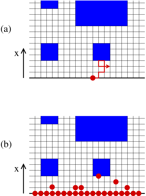
The first step of our work is to study single particle infiltration in the SCs, with starting positions randomly chosen in the axis. This is equivalent to the infiltration of non-interacting particles starting at that axis at , as proposed in a recent model of diffusion in porous deposits [40]. In one time unit, the particle randomly chooses one nearest neighbor site to jump to, and moves to that site only if it is also a pore site; otherwise, the particle does not move. Fig. 2a illustrates the first steps of a particle in SC1.
We simulated single particle RWs in the stages to of SC1 and of SC2. The maximal time of each walk was in the largest lattices. These conditions ensure that no walker reaches the border at .
The model of diffusive infiltration in the SCs is defined analogously to the model in planar and cubic lattices shown in Ref. [36]. The axis (line ) is permanently filled with mobile particles that execute RWs with excluded volume interactions, i. e. with at most one particle per site. In one time unit, each particle executes an average of one step trial to a randomly chosen nearest neighbor site. The step is allowed if the target site is a pore site and is not occupied by another diffusing particle; otherwise, the particle does not move. If a particle leaves the axis, another particle immediately refills the available position. This creates a pressure for the particles to move to the positive direction. Fig. 2b illustrates the beginning of this process in SC1.
In our simulations, independent configurations of diffusive infiltration were generated in stages of SC1 and of SC2, with maximal times . Simulations in of SC1 were also performed to confirm the absence of finite-size effects.
The generators of the MSs studied here are shown in Figs. 1c and 1d; these fractals are respectively called MS1 and MS2. Those images differ from usual presentations of these fractals because they highlight the solid region (dark) of the generator, with the remaining region being the porous one. The fractal dimensions of the porous regions are for MS1 and for MS2. The values up to five decimal places are also shown in Table 1.
| Fractal | (simulation) | (simulation) | |||
| SC1 | (Ref. [8]) | ||||
| SC2 | (Ref. [8]) | ||||
| MS1 | |||||
| MS2 |
Lattice sites are located at the vertices of the cubes produced at each step of the construction of the MS and the distance between nearest neighbor sites is taken as the size unit. At stage , the lateral size of the lattice is , where is the scaling factor of the generator. The solid sites are located inside the lacunas at each stage and the remaining sites are pore sites, which may be occupied by particles executing RWs. An impenetrable border of the MS lattice is located at the plane () and periodic conditions are considered in the directions and .
In single particle infiltration in MSs, each particle is released at a randomly chosen pore site of the border ( plane) and, in each time unit, chooses one nearest neighbor site and jumps to that site only if it is also a pore site. RWs were generated in stages of MS1 and of MS2, with .
In diffusive infiltration in MSs, all pore sites of the border are permanently occupied by mobile particles and each particle executes an average of one step trial per unit time; when a pore site at becomes empty, it is instantaneously refilled. In stages of MS1 and of MS2, we produced configurations of diffusive infiltration, with maximal times .
A diffusion front is defined in the diffusive infiltration problem. The front height at position of a SC [ of a MS] is an average of the displacements of all particles with that position. In general, at a given substrate position , the front height is
| (4) |
where is the number of particles with that substrate position and runs over all those particles. If this definition is used for a configuration with no vacancy between particles (solid-on-solid aggregates), then is equal to the position of the top particle at position ; this is the usual definition of the interface in film growth and/or kinetic roughening models, and justifies the factor in Eq. 4.
The roughness of the diffusion front, , was calculated for selected times. It is defined as the rms fluctuation of , averaged over the substrate positions and over different configurations of the front at time . Finite-size effects on are expected only when or longer, where is the dynamical exponent of the front roughening [41]. However, the infiltration simulations are restricted to , thus is not expected to depend on , i. e. roughening is in the growth regime [41].
III Simulation results
III.1 Infiltration in Sierpinski carpets
Fig. 3 shows the time evolution of the mean square displacement in the direction in single particle diffusion in SC1 () and SC2 (). The linear fits of each data set are shown.

The mean square displacement oscillates in both cases, but the oscillations are visible only in the data for SC2. The diffusing particle may take a long time to go around the border of lacunas, whose sizes increase as the particle travels to more distant points. The amplitude of oscillations are much smaller in SC1 because its lacunas are relatively small if compared to those of SC2. These oscillations are log-periodic, similarly to those observed in simulations of RWs in the bulk of SCs [14], and are consequence of the discrete scale invariance of those fractals [42, 43].
The estimates for SC1 and for SC2 are obtained by performing linear fits in several time ranges in the simulated interval. Fits of the data in smaller stages of construction of those fractals confirm that finite-size effects are negligible.
These estimates are very close to those obtained from simulations of RWs starting at random points of the bulk of the SCs: [8] and [9, 19] in SC1; [12] and [8] in SC2. This comparison is important because it shows that the long time properties of single particle RWs in the SCs do not depend on the initial positions of those particles nor on the boundary conditions. We understand that this is consistent with the uniqueness of Brownian motion in a Sierpinski carpet demonstrated in Ref. [15], which is related to the uniqueness of the Laplacian definition in that fractal. The most accurate estimates of for each fractal are shown in Table 1.
The diffusive infiltration in SC1 is illustrated in Fig. 4a, which shows a region near the filled border of that lattice at time . Fig. 4a also shows an averaged diffusion front , in which (position , with integer ) is the average of the heights (Eq. 4) from to . This is an average over substrate positions, which is the second smallest size of the lacunas in the lattice. This averaging highlights the long wavelength fluctuations. Instead, the diffusion front , which is shown in Fig. 4b, also has short wavelength fluctuations of large amplitude.

The averaged diffusion front has a structure of rounded mounds separated by gaps, with the mounds located between the third level lacunas. The main depletion of that front is close to the fourth level lacuna (the largest one at the left side). This morphology resembles that observed in infiltration of glycerin in the Hele-Shaw cells in Ref. [34], which reinforces the connection with that system. The experimental front is smoother, but this is probably related to interfacial tension effects and to the small stage of the SC used in the cell.
The filling is the number of moving particles at time per lattice site. Fig. 5 shows the time evolution of in SC1 () and SC2 () and linear fits of each data set. Considering fits in various time ranges, we obtain the estimates and , respectively, which are reproduced in Table 1.

The value of in SC1 is very close to the estimate of Ref. [33] for infiltration simulated with a diffusion equation; in SC2, was obtained in that work, which differs from our estimate. The experiments of glycerin infiltration in the Hele-Shaw cells of Ref. [34] give and , respectively, which are both in excellent agreement with our results. These results suggest a universal scaling in the diffusive infiltration problem in SCs.
The exponents are much smaller than the estimates of in the same SCs. The differences are for SC1 and for SC2, both much larger than error bars of the estimates of both exponents.
We also performed simulations of single particle RWs and of diffusive infiltration in free square lattices, i. e. without obstacles. Even with a small number of configurations in a lattice of lateral size and with maximal simulation time , we obtained with good accuracy.
III.2 Infiltration in Menger sponges
Fig. 6 shows the time evolution of the mean square displacement in the direction of single particle diffusion in MS1 () and MS2 (), with linear fits of each data set. The log-periodic oscillations due to the discrete scale invariance [14, 42] are also observed here, and their amplitudes are also larger in the fractal with larger lacunas (MS2).


Fits of the data in various time intervals yield the estimates for MS1 and for MS2, which are also reproduced in Table 1. Previous estimates of in MSs were obtained only from lower and upper bounds [7, 18], thus they had lower accuracy than the present ones. Simulations in smaller stages of MS1 and MS2 give approximately the same estimates, indicating that finite-size effects are small.
Note that the exponent in the MSs follows the same trend of decrease with the fractal dimension that was observed in the SCs in Ref. [9]. Moreover, those exponents are near the normal diffusion value , which is also observed in fractals without dead ends and dimensions between and , such as the SCs [12].
The diffusive infiltration is illustrated in Figs. 7a,b, which show cross sections of MS1 near the filled boundary at . In the plane (Fig. 7a), the density of obstacles near the filled boundary is low, thus it is easier for particles to reach larger distances. In the plane (Fig. 7b), the density of blocks near the boundary is large, which confines many particles; however, note that three particles have already reached an upper porous region of this plane by migrating through other planes.
Fig. 8 shows the time evolution of the filling in MS1 () and MS2 (). Linear fits of the data with are shown. We also analyzed fits in different time ranges to obtain the estimates and , respectively. They are presented in Table 1. Again, we also observe that the exponents and are very different.

We also simulated single particle RWs and the diffusive infiltration model in simple cubic lattices. With a small number of configurations and maximal time , we obtained , which is consistent with normal diffusion in both cases.
IV Scaling approach
A scheme of the diffusive infiltration in a fractal is shown in Fig. 9, with a characteristic length filled by the diffusing species. is the lateral size of the lattice, whose dimension is and whose filled boundary has dimension . For SCs, the boundary is a filled line, thus ; for MS2, the boundary is a plane, thus ; however, for MS1, the filled boundary has the geometry of SC1, thus it has dimension .
The diffusing front is expected to advance with the same scaling of single particle diffusion because the more advanced particles move in a region with low density, in which the main constraints are the irregularities of the fractal network and not the excluded volume interactions. For this reason, we expect
| (5) |
The value of calculated in our simulations are consistent with this scaling, but fluctuations are much larger than those of single particle diffusion.

The filled region can be divided in hypercubes of edge ; one of them is highlighted in Fig. 9. The total filling of each hypercube is
| (6) |
assuming that is sufficiently large for the fractality of the medium to be observed. If , the number of hypercubes in the boundary is
| (7) |
The total filling consequently scales as
| (8) |
This gives an exact relation between the single particle diffusion exponent and the diffusive infiltration exponent:
| (9) |
where Eq. (2) was also used.
Table 1 shows the values of obtained from the best available estimates of and the exact dimensions and . They are in excellent agreement with the estimates of obtained in simulations. Note that Eq. 9 implies for systems in which bulk and boundary are regular lattices with integer dimensions, since and single particle diffusion is normal in those cases. Also note that the successful application to systems whose boundaries are compact (SCs and MS2) and fractal (MS1) is a strong support to this scaling approach.
In Ref. [9], it was shown that the exponent in SCs has an approximately linear dependence on if this dimension is not much smaller than . Combination of this relation with Eq. (9) gives an approximately quadratic dependence of on . Indeed, such a quadratic relation was obtained by Filipovitch et al [34] in the experiments of fluid infiltration in SCs. For many other fractals in which the RW exponent is known, Eq. 9 can predict the anomalous properties of diffusive infiltration and, if experiments are available, it may help to evaluate the applicability of a given fractal model.
V Roughening of the infiltration fronts
The roughness of the diffusion front was measured in all fractals at selected times, from to in SCs and from to in MSs. Fig. 10a shows as a function of in SC1, MS1, and in the square lattice; Fig. 10b shows the same quantities in SC2, MS2, and in the simple cubic lattice.

In square and cubic lattices, the linear fits of the data shown in Figs. 10a,b give with a growth exponent . The movement of the particles in the diffusion front is completely random, thus the height of each position in the SCs ( in MSs) randomly fluctuates around the average value . This is characteristic of random uncorrelated deposition, in which [41]. Since in diffusive infiltration in those lattices, we obtain , which is consistent with the simulation results.
The infiltration problem defined here has similarities with that of gradient percolation, in particular the existence of lattice borders with fixed concentration of particles; see e. g. Ref. [36]. However, a very important difference is the existence of a fixed concentration gradient along the direction in that case; instead, in the present problem, the concentration gradient is continuously varying between the filled border and the diffusion front. In the gradient percolation problem, the diffusion front is defined as the interface of a cluster of connected particles, which also differs from the present definition. Thus, even if correlations in particle positions were introduced in our model (e. g. to represent surface tension effects), the roughening might be different from that of the gradient percolation front [38, 39].
Despite the simplicity of the diffusive infiltration front in regular lattices and the fact that the uncorrelated growth extends to the fractal media, some interesting features can be observed in the latter case. As shown in Figs. 10a,b, the roughness oscillates in all fractals. As the front reaches the lower borders of a set of parallel lacunas of a given size, the front can advance only in the regions between those lacunas, which leads to large differences in the heights at the confined and at the non-confined regions; see e. g. Figs. 4a and 7a,b. However, when the front reaches the upper borders of those lacunas, it enters a more homogeneous region, in which lateral diffusion slows down the increase of height differences.
This effect is enhanced in lattices with large lacunas, which is the case of SC2 and MS2. For instance, Figs. 11a shows an infiltration profile in SC2 at , in which the front has bypassed the second level lacunas but did not reach the larger ones. Correspondingly, Fig. 10b shows a plateau in the plot at . On the other hand, Fig. 11b shows an infiltration profile at , in which particles enter the gaps between the third level lacunas. Correspondingly, Fig. 10b shows a rapid increase of at . The main contribution to the roughness is that from the long wavelength fluctuations, which are the height differences between the evolving regions (in the gaps) and the blocked regions (below the large lacunas). This is not a kinetic roughening feature, but an effect of the channeled geometry of the medium. For this reason, it is meaningful to estimate a growth exponent in these cases.

The roughness oscillations are also log-periodic, which is related to the discrete scale invariance of the medium. An important feature is that the periods have approximately the same value for the fractals with the same scaling factors in the generators, even having very different and different embedding dimensions: for SC1 and MS1 (Fig. 10a) and for SC2 and MS2 (Fig. 10b). The relevance of the scaling factor of the generator is consistent with the approach of Ref. [42] to explain these oscillations in kinetic models.
Other growth models have also been studied in substrates with the geometry of SCs [44, 45, 46, 47]. The roughness oscillations were also observed in the simulations of ballistic deposition in SCs [44]. However, a comparison with our results is not possible because the front kinetics and the substrate effects are very different. For instance, here the front grows in the plane in which the SC is embedded, thus it finds different disordered environments in the lateral directions during the growth, while those works consider growth parallel to the SC plane, so that the lateral disorder is the same for the growing columns at all heights.
VI Conclusion
Although diffusion in deterministic fractals have been intensively studied since a long time, as reviewed in Refs. [2, 4], novel interesting features and applications frequently appear, as shown in recent works, e. g. Refs. [18, 16, 17, 43, 48, 49, 50]. The simulation of infiltration of a diffusing fluid in a Sierpinski carpet and subsequent experimental realization of this process in a Hele-Shaw cell provide a very interesting macroscopic illustration of that phenomena [33, 34]. However, the significant discrepancy between the anomalous exponent of filled area and the exponent of single particle diffusion in the same fractals was not explained. The main aim of this work was to fill this gap.
We performed numerical simulations of the infiltration of randomly moving particles from a permanently filled border in deterministic fractals embedded in dimensions and , viz. Sierpinski carpets (SCs) and Menger sponges (MSs). The exponent of the time scaling of the infiltrated area/volume was measured and confirms the accuracy of the previous infiltration simulations [33] and experiments [34], which were obtained in smaller stages of construction of SCs. Single particle diffusion starting from the same border was also studied numerically and the exponent of the mean square displacement scaling was measured. In SCs, the values of agree with previous estimates in the bulk of those fractals; in MSs, they improve previous estimates, since they were based only on lower and upper bounds and had large uncertainties.
A scaling approach is proposed to relate exponents and , considering the fractal dimensions of the infiltrated region and of the region from which the diffusing particles come. The numerical results are in excellent agreement with this approach. Thus, if the dimensions characterizing the porous medium and its boundaries are known, then the single particle diffusion exponent (which was calculated for a variety of fractals in more than three decades) is sufficient to determine the scaling properties in the diffusive infiltration problem.
We also showed that the roughness of the diffusion fronts has log-periodic oscillations in time, which is characteristic of random walks and other kinetic models in fractals [14, 42, 43]. The same oscillations are observed in the mean-square displacement of single particle RWs. In SCs and MSs whose generators have the same scaling factor, the periods are approximately the same, despite the very different dimensions of those fractals, which shows the relevance of the discrete scale invariance.
Acknowledgements.
The author thanks Vaughan Voller for helpful discussion. This work was supported by CNPq and FAPERJ (Brazilian agencies).References
- [1] J. P. Bouchaud and A Georges, Phys. Rep. 185, 127 (1990).
- [2] S. Havlin and D. Ben-Avraham, Adv. Phys. 36, 695 (1987); 51, 187 (2002).
- [3] R. Metzler and J. Klafter, Phys. Rep. 339, 1 (2000).
- [4] R. Metzler, J.-H. Jeon, A. G. Cherstvya, and E. Barkaid, Phys. Chem. Chem. Phys. 16, 24128 (2014).
- [5] P. Xu, Fractals 23, 1530001 (2015).
- [6] B. B. Mandelbrot, The Fractal Geometry of Nature (Freeman, San Francisco, 1982).
- [7] D. Ben-Avraham and S. Havlin, J. Phys. A: Math. Gen. 16, L559 (1983).
- [8] M. H. Kim, D. H. Yoon, and I. Kim, J. Phys. A: Math. Gen. 26, 5655 (1993).
- [9] F. D. A. Aarão Reis, J. Phys. A: Math. Gen. 28, 6277 (1995).
- [10] R. Dasgupta, T. K. Ballabh, and S. Tarafdar, J. Phys. A: Math. Gen. 32, 6503 (1999).
- [11] F. D. A. Aarão Reis, Phys. Lett. A 214, 239 (1996).
- [12] F. D. A. Aarão Reis, J. Phys. A: Math. Gen. 29, 7803 (1996).
- [13] J.-W. Kim, E. Perfect, and H. Choi, Water Resour. Res. 43, W01405 (2007).
- [14] M. A. Bab, G. Fabricius, and E. V. Albano, J. Chem. Phys. 128, 044911 (2008).
- [15] M. T. Barlow, R. F. Bass, T. Kumagai, and A. Teplyaev, J. Eur. Math. Soc. 12, 655 (2010).
- [16] R. Haber, J. Prehl, H. Herrmann, and K. H. Hoffmann, Phys. Lett. A 377, 2840 (2013).
- [17] Z. Darázs, A. Anishchenko, T. Kiss, A. Blumen, and Oliver Mülken, Phys. Rev. E 90, 032113 (2014).
- [18] A. S. Balankin, Phys. Rev. E 92, 062146 (2015).
- [19] O. Suwannasen, M. A. Allen, and J. C. Sprott, ScienceAsia 42, 33 (2016).
- [20] M. Küntz and P. Lavallée, J. Phys. D: Appl. Phys. 34, 2547 (2001).
- [21] E. Gerolymatou, I. Vardoulakis, and R. Hilfer, J. Phys. D: Appl. Phys. 39, 4104 (2006).
- [22] E. Stalgorova and T. Babadagli, Physica A 405, 181 (2014).
- [23] C. Atzeni, G. Pia, U. Sanna, and N. Spanu, Constr. Build. Mater. 22, 1607 (2008).
- [24] D. Roubinet, J.-R. de Dreuzy, and D. M. Tartakovsky, Computers and Geosciences 50, 52 (2013).
- [25] N. S. Martys, Phys. Rev. E 50, 335 (1994).
- [26] E. Perfect, R. W. Gentry, M. C. Sukop, and J. E. Lawson, Geoderma 134, 240 (2006).
- [27] M. Dentz and D. M. Tartakovsky, Geophys. Res. Lett. 33, L16406 (2006).
- [28] M. Persson, H. Yasuda, J. Albergel, R. Berndtsson, P. Zante, S. Nasri, and P. Ohrstrom, J. Hydrol. 250, 98 (2001).
- [29] D. A. Lockington and J.-Y. Parlange, J. Phys. D: Appl. Phys. 36, 760 (2003).
- [30] P. Xu and B. Yu, J. Appl. Phys. 100, 104906 (2006).
- [31] A. Bru and J. M. Pastor, Geoderma 134, 295 (2006).
- [32] D. N. Gerasimov, V. A. Kondratieva, and O. A. Sinkevich, Physica D 239, 1593 (2010).
- [33] V. Voller, Water Resour. Res. 51, 2119 (2015).
- [34] N. Filipovitch, K. M. Hill, Al. Longjas, and V. R. Voller, Water Resour. Res. 52, 5167 (2016).
- [35] V. R. Gisladottir, D. Roubinet, and D. M. Tartakovsky, Transp. Porous Med., 115, 311 (2016).
- [36] J. F. Gouyet, M. Rosso, and B. Sapoval, Fractal Surfaces and Interfaces, in Fractals and Disordered Systems, Second Edition, eds. A. Bunde and S. Havlin (Springer, Berlim-Heidelberg, 1996). doi:10.1007/978-3-642-84868-1
- [37] B. Sapoval, M. Rosso, and J. F. Gouyet, J. Phys. (Paris), Lett. 46, L149 (1985).
- [38] A. Bunde and J. F. Gouyet, J. Phys. A 18, L285 (1985).
- [39] M. Rosso, and J. F. Gouyet, and B. Sapoval, Phys. Rev. Lett. 57, 3195 (1986).
- [40] F. D. A. Aarão Reis and D. di Caprio, Phys. Rev. E 89, 062126 (2014).
- [41] A. L. Barabási and H. E. Stanley, Fractal concepts in surface growth (Cambridge University Press, Cambribge, England, 1995).
- [42] M. A. Bab, G. Fabricius, and E. V. Albano, EPL 81, 10003 (2008).
- [43] E. Akkermans, O. Benichou, G. V. Dunne, A. Teplyaev, and R. Voituriez, Phys. Rev. E 86, 061125 (2012).
- [44] C. M. Horowitz, F. Romá, and E. V. Albano, Phys. Rev. E 78, 061118 (2008).
- [45] S. B. Lee, H.-C. Jeong, and J. M. Kim, J. Korean Phys. Soc. 58, 1076 (2011).
- [46] G. Tang, Z. P. Xun, R. J. Wen, K. Han, H. Xia, D. P. Hao, W. Zhou, X. Q. Yang, and Y. L. Chen, Physica A 389, 4552 (2010).
- [47] Z. Xun, G. Tang, L. Song, K. Han, H. Xia, D. Hao, and Y. Yang, J. Stat. Mech. P12008 (2014).
- [48] G. Forte, F. Cecconi, and A. Vulpiani, Eur. Phys. J. B 87, 102 (2014).
- [49] T. Miyaguchi and T. Akimoto, Phys. Rev. E 91, 010102(R) (2015).
- [50] I. M. Sokolov, J. Phys. A: Math. Theor. 49, 095003 (2016).