Wasserstein Learning of Deep Generative Point Process Models

Let $S$ be a compact space equipped with a Borel $\sigma$-algebra $\mathcal{B}$. Take $\Xi$ as the set of counting measures on $S$ with $\mathcal{C}$ as the smallest $\sigma$-algebra on it. Let $(\Omega,\mathcal{F},\mathbb{P})$ be a probability space. A point process on $S$ is a measurable map $\xi:\Omega\to\Xi$ from the probability space $(\Omega,\mathcal{F},\mathbb{P})$ to the measurable space $(\Xi,\mathcal{C})$. Figure 1-a illustrates this mapping.

Every realization of a point process $\xi$ can be written as $\xi=\sum_{i=1}^{n}\delta_{X_{i}}$ where $\delta$ is the Dirac measure, $n$ is an integer-valued random variable and $X_{i}$’s are random elements of $S$ or events. A point process can be equivalently represented by a counting process: $N(B):=\int_{B}\xi(x)dx$, which basically is the number of events in each Borel subset $B\in\mathcal{B}$ of $S$. The mean measure $M$ of a point process $\xi$ is a measure on $S$ that assigns to every $B\in\mathcal{B}$ the expected number of events of $\xi$ in $B$, i.e., $M(B):=\mathbb{E}[N(B)]$ for all $B\in\mathcal{B}$.

For inhomogeneous Poisson process, $M(B)=\int_{B}\lambda(x)dx$, where the intensity function $\lambda(x)$ yields a positive measurable function on $S$. Intuitively speaking, $\lambda(x)dx$ is the expected number of events in the infinitesimal $dx$. For the most common type of point process, a Homogeneous Poisson process, $\lambda(x)=\lambda$ and $M(B)=\lambda|B|$, where $|\cdot|$ is the Lebesgue measure on $(S,\mathcal{B})$. More generally, in Cox point processes, $\lambda(x)$ can be a random density possibly depending on the history of the process. For any point process, given $\lambda(\cdot)$, $N(B)\sim\text{Poisson}(\int_{B}\lambda(x)dx)$. In addition, if $B_{1},\ldots,B_{k}\in\mathcal{B}$ are disjoint, then $N(B_{1}),\ldots,N(B_{k})$ are independent conditioning on $\lambda(\cdot)$.

For the ease of exposition, we will present the framework for the case where the events are happening in the real half-line of time. But the framework is easily extensible to the general space.

A particularly interesting case of point processes is given when $S$ is the time interval $[0,T)$, which we will call a temporal point process. Here, a realization is simply a set of time points: $\xi=\sum_{i=1}^{n}\delta_{t_{i}}$. With a slight notation abuse we will write $\xi=\{t_{1},\ldots,t_{n}\}$ where each $t_{i}$ is a random time before $T$. Using a conditional intensity (rate) function is the usual way to characterize point processes.

For Inhomogeneous Poisson process (IP), the intensity $\lambda(t)$ is a fixed non-negative function supported in $[0,T)$. For example, it can be a multi-modal function comprised of $k$ Gaussian kernels: $\lambda(t)=\sum_{i=1}^{k}\alpha_{i}(2\pi\sigma_{i}^{2})^{-1/2}\exp\left(-(t-c_{i})^{2}/\sigma_{i}^{2}\right),$ for $t\in[0,T)$, where $c_{i}$ and $\sigma_{i}$ are fixed center and standard deviation, respectively, and $\alpha_{i}$ is the weight (or importance) for kernel $i$.

A self-exciting (Hawkes) process (SE) is a cox process where the intensity is determined by previous (random) events in a special parametric form: $\lambda(t)=\mu+\beta\sum_{t_{i}<t}g(t-t_{i}),$ where $g$ is a nonnegative kernel function, e.g., $g(t)=\exp(-\omega t)$ for some $\omega>0$. This process has an implication that the occurrence of an event will increase the probability of near future events and its influence will (usually) decrease over time, as captured by (the usually) decaying fixed kernel $g$. $\mu$ is the exogenous rate of firing events and $\alpha$ is the coefficient for the endogenous rate.

In contrast, in self-correcting processes (SC), an event will decrease the probability of an event: $\lambda(t)=\exp(\eta t-\sum_{t_{i}<t}\gamma).$ The $\exp$ ensures that the intensity is positive, while $\eta$ and $\gamma$ are exogenous and endogenous rates.

We can utilize more flexible ways to model the intensity, e.g., by a Recurrent Neural Network (RNN): $\lambda(t)=g_{w}(t,h_{t_{i}}),$ where $h_{t_{i}}$ is the feedback loop capturing the influence of previous events (last updated at the latest event) and is updated by $h_{t_{i}}=h_{v}(t_{i},h_{t_{i-1}})$. Here $w$, $v$ are network weights.

Given samples from a point process, one way to estimate the process is to find a model $(\Omega_{g},\mathcal{F}_{g},\mathbb{P}_{g})\to(\Xi,\mathcal{C})$ that is close enough to the real data $(\Omega_{r},\mathcal{F}_{r},\mathbb{P}_{r})\to(\Xi,\mathcal{C})$. As mentioned in the introduction, Wasserstein distance [19] is our choice as the proximity measure. The Wasserstein distance between distribution of two point processes is:

where $\Psi(\mathbb{P}_{r},\mathbb{P}_{g})$ denotes the set of all joint distributions $\psi(\xi,\rho)$ whose marginals are $\mathbb{P}_{r}$ and $\mathbb{P}_{g}$.

The distance between two sequences $\|\xi-\rho\|_{\star}$, is tricky and need further attention. Take $\xi=\{x_{1},x_{2},\ldots,x_{n}\}$ and $\rho=\{y_{1},\ldots,y_{m}\}$, where for simplicity we first consider the case $m=n$. The two sequences can be thought as discrete distributions $\mu^{\xi}=\sum_{i=1}^{n}\frac{1}{n}\delta_{x_{i}}$ and $\mu^{\rho}=\sum_{i=1}^{n}\frac{1}{n}\delta_{y_{i}}$. Then, the distance between these two is an optimal transport problem $\mathop{\mathrm{argmin}}_{\pi\in\Sigma}\langle\pi,C\rangle$, where $\Sigma$ is the set of doubly stochastic matrices (rows and columns sum up to one), $\langle\cdot,\cdot\rangle$ is the Frobenius dot product, and $C$ is the cost matrix. $C_{ij}$ captures the energy needed to move a probability mass from $x_{i}$ to $y_{j}$. We take $C_{ij}=\|x_{i}-y_{j}\|_{\circ}$ where $\|\cdot\|_{\circ}$ is the norm in $S$. It can be seen that the optimal solution is attained at extreme points and, by Birkhoff’s theorem, the extreme points of the set of doubly stochastic matrices is a permutation [21]. In other words, the mass is transfered from a unique source event to a unique target event. Therefore, we have: $\|\xi-\rho\|_{\star}=\min_{\sigma}\sum_{i=1}^{n}\|x_{i}-y_{\sigma(i)}\|_{\circ},$ where the minimum is taken among all $n!$ permutations of $1\ldots n$. For the case $m\neq n$, without loss of generality we assume $n\leq m$ and define the distance as follows:

where $s$ is a fixed limiting point in border of the compact space $S$ and the minimum is over all permutations of $1\ldots m$. The second term penalizes unmatched points in a very special way which will be clarified later. Appendix B proves that it is indeed a valid distance measure.

Interestingly, in the case of temporal point process in $[0,T)$ the distance between $\xi=\left\{t_{1},\ldots,t_{n}\right\}$ and $\rho=\left\{\tau_{1},\ldots,\tau_{m}\right\}$ is reduced to

where the time points are ordered increasingly, $s=T$ is chosen as the anchor point, and $|\cdot|$ is the Lebesgue measure in the real line. A proof is given in Appendix C. This choice of distance is significant in two senses. First, it is computationally efficient and no excessive computation is involved. Secondly, in terms of point processes, it is interpreted as the volume by which the two counting measures differ. Figure 1-b demonstrates this intuition and justifies our choice of metric in $\Xi$ and Appendix D contains the proof.

Equation (1) is computationally highly intractable and its dual form is usually utilized [19]:

where the supremum is taken over all Lipschitz functions $f:\Xi\to\mathbb{R}$, i.e., functions that assign a value to a sequence of events (points) and satisfy $|f(\xi)-f(\rho)|\leq\|\xi-\rho\|_{\star}$ for all $\xi$ and $\rho$.

However, solving the dual form is still highly nontrivial. Enumerating all Lipschitz functions over point process realizations is impossible. Instead, we choose a parametric family of functions to approximate the search space $f_{w}$ and consider solving the problem

where $w\in\mathcal{W}$ is the parameter. The more flexible $f_{w}$, the more accurate will be the approximation.

It is notable that W-distance leverages the geometry of the space of event sequences in terms of their distance, which is not the case for MLE-based approach. It in turn requires functions of event sequences $f(x_{1},x_{2},...)$, rather than functions of the time stamps $f(x_{i})$. Furthermore, Stein’s method to approximate Poisson processes [22, 23] is also relevant as they are defining distances between a Poisson process and an arbitrary point process.

Equipped with a way to approximately compute the Wasserstein distance, we will look for a model $\mathbb{P}_{r}$ that is close to the distribution of real sequences. Again, we choose a sufficiently flexible parametric family of models, $g_{\theta}$ parameterized by $\theta$. Inspired by GAN [14], this generator takes a noise and turns it into a sample to mimic the real samples. In conventional GAN or WGAN, Gaussian or uniform distribution is chosen. In point processes, a homogeneous Poisson process plays the role of a non-informative and uniform-like distribution: the probability of events in every region is independent of the rest and is proportional to its volume. Define the noise process as $(\Omega_{z},\mathcal{F}_{z},\mathbb{P}_{z})\to(\Xi,\mathcal{C})$, then $\zeta\sim\mathbb{P}_{z}$ is a sample from a Poisson process on $S=[0,T)$ with constant rate $\lambda_{z}>0$. Therefore, $g_{\theta}:\Xi\to\Xi$ is a transformation in the space of counting measures. Note that $\lambda_{z}$ is part of the prior knowledge and belief about the problem domain. Therefore, the objective of learning the generative model can be written as $\min W(\mathbb{P}_{r},\mathbb{P}_{g})$ or equivalently:

In GAN terminology $f_{w}$ is called the discriminator and $g_{\theta}$ is known as the generator model. We estimate the generative model by enforcing that the sample sequences from the model have the same distribution as training sequences. Given $L$ samples sequences from real data $\mathcal{D}_{r}=\left\{\xi_{1},\ldots,\xi_{L}\right\}$ and from the noise $\mathcal{D}_{z}=\left\{\zeta_{1},\ldots,\zeta_{L}\right\}$ the two expectations are estimated empirically: $\mathbb{E}_{\xi\sim\mathbb{P}_{r}}[f_{w}(\xi)]=\frac{1}{L}\sum_{l=1}^{L}f_{w}(\xi_{l})$ and $\mathbb{E}_{\zeta\sim\mathbb{P}_{z}}[f_{w}(g_{\theta}(\zeta))]=\frac{1}{L}\sum_{l=1}^{L}f_{w}(g_{\theta}(\zeta_{l}))$.

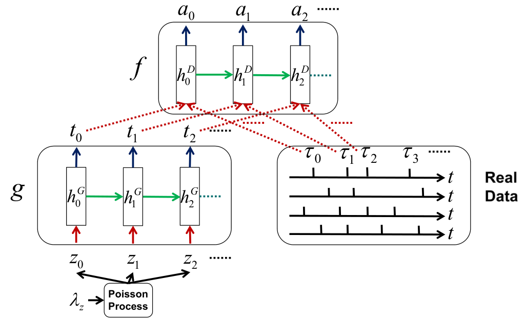
To proceed with our point process based WGAN, we need the generator function $g_{\theta}:\Xi\to\Xi$, the discriminator function $f_{w}:\Xi\to\mathbb{R}$, and enforce Lipschitz constraint on $f_{w}$. Figure 4 in Appendix A illustrates the data flow for WGANTPP.

The generator transforms a given sequence to another sequence. Similar to [24, 25] we use Recurrent Neural Networks (RNN) to model the generator. If the input and output sequences are $\zeta=\left\{z_{1},\ldots,z_{n}\right\}$ and $\rho=\left\{t_{1},\ldots,t_{n}\right\}$ then the generator $g_{\theta}(\zeta)=\rho$ works according to

Here $h_{i}$ is the $k$-dimensional history embedding vector and $\phi^{h}_{g}$ and $\phi^{x}_{g}$ are the activation functions. The parameter set of the generator is $\theta=\left\{\left(A^{h}_{g}\right)_{k\times 1},\left(B^{h}_{g}\right)_{k\times k},\left(b^{h}_{g}\right)_{k\times 1},\left(B^{x}_{g}\right)_{1\times k},\left(b^{x}_{g}\right)_{1\times 1}\right\}.$ Similarly, we define the discriminator function who assigns a scalar value $f_{w}(\rho)=\sum_{i=1}^{n}a_{i}$ to the sequence $\rho=\left\{t_{1},\ldots,t_{n}\right\}$ according to

where the parameter set is comprised of $w=\left\{\left(A^{h}_{d}\right)_{k\times 1},\left(B^{h}_{d}\right)_{k\times k},\left(b^{h}_{d}\right)_{k\times 1},\left(B^{a}_{d}\right)_{1\times k},\left(b^{a}_{d}\right)_{1\times 1}\right\}.$ Note that both generator and discriminator RNNs are causal networks. Each event is only influenced by the previous events. To enforce the Lipschitz constraints the original WGAN paper [12] adopts weight clipping. However, our initial experiments shows an inferior performance by using weight clipping. This is also reported by the same authors in their follow-up paper [20] to the original work. The poor performance of weight clipping for enforcing 1-Lipschitz can be seen theoretically as well: just consider a simple neural network with one input, one neuron, and one output: $f(x)=\sigma(wx+b)$ and the weight clipping $w<c$. Then,

It is clear that when $1/|\sigma^{\prime}(wx+b)|<c$, which is quite likely to happen, the Lipschitz constraint is not necessarily satisfied. In our work, we use a novel approach for enforcing the Lipschitz constraints, avoiding the computation of the gradient which can be costly and difficult for point processes. We add the Lipschitz constraint as a regularization term to the empirical loss of RNN.

We can take each of the $2L\choose 2$ pairs of real and generator sequences, and regularize based on them; however, we have seen that only a small portion of pairs ($O(L)$), randomly selected, is sufficient. The procedure of WGANTPP learning is given in Appendix E

Remark The significance of Lipschitz constraint and regularization (or more generally any capacity control) is more apparent when we consider the connection of W-distance and optimal transport problem [21]. Basically, minimizing the W-distance between the empirical distribution and the model distribution is equivalent to a semidiscrete optimal transport [21]. Without capacity control for the generator and discriminator, the optimal solution simply maps a partition of the sample space to the set of data points, in effect, memorizing the data points.

Synthetic datasets. We simulate 20,000 sequences over time $[0,T)$ where $T=15$, for inhomogeneous process (IP), self-exciting (SE), and self-correcting process (SC), recurrent neural point process (NN). We also create another 4 ($=C_{4}^{3}$) datasets from the above 4 synthetic data by a uniform mixture from the triplets. The new datasets IP+SE+SC, IP+SE+NN, IP+SC+NN, SE+SC+NN are created to testify the mode dropping problem of learning a generative model. The parameter setting follows:

i) Inhomogeneous process. The intensity function is independent from history and given in Sec. 2.2, where $k=3,\alpha=[3,7,11],c=[1,1,1],\sigma=[2,3,2]$.
ii) Self-exciting process. The past events increase the rate of future events. The conditional intensity function is given in Sec. 2.2 where $\mu=1.0,\beta=0.8$ and the decaying kernel $g(t-t_{i})=e^{-(t-t_{i})}$.
iii) Self-correcting process. The conditional intensity function is defined in Sec. 2.2. It increases with time and decreases by events occurrence. We set $\eta=1.0,\gamma=0.2$.
iv) Recurrent Neural Network process. The conditional intensity is given in Sec. 2.2, where the neural network’s parameters are set randomly and fixed. We first feed random variable from [0,1] uniform distribution, and then iteratively sample events from the intensity and feed the output into the RNN to get the new intensity for the next step.

Real datasets. We collect sequences separately from four public available datasets, namely, health-care MIMIC-III, public media MemeTracker, NYSE stock exchanges, and publications citations. The time scale for all real data are scaled to [0,15], and the details are as follows:

i) MIMIC. MIMIC-III (Medical Information Mart for Intensive Care III) is a large, publicly available dataset, which contains de-identified health-related data during 2001 to 2012 for more than 40,000 patients. We worked with patients who appear at least 3 times, which renders 2246 patients. Their visiting timestamps are collected as the sequences.
ii) Meme. MemeTracker tracks the meme diffusion over public media, which contains more than 172 million news articles or blog posts. The memes are sentences, such as ideas, proverbs, and the time is recorded when it spreads to certain websites. We randomly sample 22,000 cascades.
iii) MAS. Microsoft Academic Search provides access to its data, including publication venues, time, citations, etc. We collect citations records for 50,000 papers.
iv) NYSE. We use 0.7 million high-frequency transaction records from NYSE for a stock in one day. The transactions are evenly divided into 3,200 sequences with equal durations.

Details. The WGAN generator and discriminator are both RNNs with 64 hidden neurons without batch normalization, and the activation function is tanh. The Adam optimization method with learning rate 1e-4, $\beta_{1}=0.5,\beta_{2}=0.9$, is applied and the batch size is 256.

Baselines. We compare the proposed method of learning point processes (i.e., minimizing sample distance) with maximum likelihood based methods for point process. To use MLE inference for point process, we have to specify its parametric model. The used parametric model are inhomogeneous Poisson process (mixture of Gaussian), self-exciting process, self-correcting process, and RNN. For each data, we use all the above solvers to learn the model and generate new sequences, and then we compare the generated sequences with real ones.

Evaluation metrics. Although our model is an intensity-free approach we will evaluate the performance by metrics that are computed via intensity. For all models, we work with the empirical intensity instead. Note that our objective measures are in sharp contrast with the best practices in GANs in which the performance is usually evaluated subjectively, e.g., by visual quality assessment. We evaluate the performance of different methods to learn the underlying processes via two measures: 1) The first one is the well-known QQ plot of sequences generated from learned model. The quantile-quantile (q-q) plot is the graphical representation of the quantiles of the first data set against the quantiles of the second data set. From the time change property [7] of point processes, if the sequences come from the point process $\lambda(t)$ , then the integral $\Lambda=\int_{t_{i}}^{t_{t+1}}\lambda(s)ds$ between consecutive events should be exponential distribution with parameter 1. Therefore, the QQ plot of $\Lambda$ against exponential distribution with rate 1 should fall approximately along a 45-degree reference line. The evaluation procedure is as follows: i) The ground-truth data is generated from a model, say IP; ii) All 5 methods are used to learn the unknown process using the ground-truth data; iii) The learned model is used to generate a sequence; iv) The sequence is used against the theoretical quantiles from the model to see if the sequence is really coming from the ground-truth generator or not; v) The deviation from slope 1 is visualized or reported as a performance measure. 2) The second metric is the deviation between empirical intensity from the learned model and the ground truth intensity. We can estimate empirical intensity $\lambda^{\prime}(t)=E(N(t+\delta t)-N(t))/\delta t$ from sufficient number of realizations of point process through counting the average number of events during $[t,t+\delta t]$, where $N(t)$ is the count process for $\lambda(t)$. The $L_{1}$ distance between the ground-truth empirical intensity and the learned empirical intensity is reported as a performance measure.

Synthetic data. Figure 2 presents the learning ability of WGANTPP when the ground-truth data is generated via different types of point process. We first compare the QQ plots in the top row from the micro perspective view, where QQ plot describes the dependency between events. Red dots legend-ed with Real are the optimal QQ distribution, where the intensity function generates the sequences are known. We can observe that even though WGANTPP has no prior information about the ground-truth point process, it can estimate the model better except for the estimator that knows the parametric form of data. This is quite expected: When we are training a model and we know the parametric form of the generating model we can find it better. However, whenever the model is misspecified (i.e., we don’t know the parametric from a priori) WGANTPP outperforms other parametric forms and RNN approach. The middle row of figure 2 compares the empirical intensity. The Real line is the optimal empirical intensity estimated from the real data. The estimator can recover the empirical intensity well in the case that we know the parametric form where the data comes from. Otherwise, estimated intensity degrades considerably when the model is misspecified. We can observe our WGANTPP produces the empirical intensity better and performs robustly across different types of point process data. The fact that the empirical intensity estimated from MLE-IP method are good and QQ plots are very bad indicates the inhomogeneous Poisson process can capture the average intensity (Macro dynamics) accurately but incapable of capturing the dependency between events (Micro dynamics). To testify that WGANTPP can cope with mode dropping, we generate mixtures of data from three different point processes and use this data to train different models. Models with specified form can handle limited types of data and fail to learn from diverse data sources. The last row of figure 2 shows the learned intensity from mixtures of data. WGANTPP produces better empirical intensity than alternatives, which fail to capture the heterogeneity in data. To verify the robustness of WGANTPP, we randomly initialize the generator parameters and run 10 rounds to get the mean and std of deviations for both empirical intensity and QQ plot from ground truth. For empirical intensity, we compute the integral of difference of learned intensity and ground-truth intensity. Table 1 reports the mean and std of deviations for intensity deviation. For each estimators, we obtain the slope from the regression line for its QQ plot. Table 1 reports the mean and std of deviations for slope of the QQ plot. Compared to the MLE-estimators, WGANTPP consistently outperforms even without prior knowledge about the parametric form of the true underlying generative point process. Note that for mixture models QQ-plot is not feasible.

Real-world data. We evaluate WGANTPP on a diverse real-world data process from health-care, public media, scientific activities and stock exchange. For those real world data, the underlying generative process is unknown, previous works usually assume that they are certain types of point process from their domain knowledge. Figure 3 shows the intensity learned from different models, where Real is estimated from the real-world data itself. Table 2 reports the intensity deviation. When all models have no prior knowledge about the true generative process, WGANTPP recovers intensity better than all the other models across the data sets.

Analysis. We have observed that when the generating model is misspecified WGANTPP outperforms the other methods without leveraging the a priori knowledge of the parametric form. However, when the exact parametric form of data is known and when it is utilized to learn the parameters, MLE with this full knowledge performs better. However, this is generally a strong assumption. As we have observed from the real-world experiments WGANTPP is superior in terms of performance. Somewhat surprising is the observation that WGANTPP tends to outperform the MLE-NN approach which basically uses the same RNN architecture but trained using MLE. The superior performance of our approach compared to MLE-NN is another witness of the the benefits of using W-distance in finding a generator that fits the observed sequences well. Even though the expressive power of the estimators is the same for WGANTPP and MLE-NN, MLE-NN may suffer from mode dropping or get stuck in an inferior local minimum since maximizing likelihood is asymptotically equivalent to minimizing the Kullback-Leibler (KL) divergence between the data and model distribution. The inherent weakness of KL divergence [19] renders MLE-NN perform unstably, and the large variances of deviations empirically demonstrate this point.

References

- [1] DJ Daley and D Vere-Jones. An introduction to the theory of point processes. 2003.
- [2] Scott W Linderman and Ryan P Adams. Discovering latent network structure in point process data. In ICML, pages 1413–1421, 2014.
- [3] Wenzhao Lian, Ricardo Henao, Vinayak Rao, Joseph E Lucas, and Lawrence Carin. A multitask point process predictive model. In ICML, pages 2030–2038, 2015.
- [4] Lizhen Xu, Jason A Duan, and Andrew Whinston. Path to purchase: A mutually exciting point process model for online advertising and conversion. Management Science, 60(6):1392–1412, 2014.
- [5] Emmanuel Bacry, Iacopo Mastromatteo, and Jean-François Muzy. Hawkes processes in finance. Market Microstructure and Liquidity, 1(01):1550005, 2015.
- [6] Odd Aalen, Ornulf Borgan, and Hakon Gjessing. Survival and event history analysis: a process point of view. Springer Science & Business Media, 2008.
- [7] John Frank Charles Kingman. Poisson processes. Wiley Online Library, 1993.
- [8] Alan G Hawkes. Spectra of some self-exciting and mutually exciting point processes. Biometrika, 1971.
- [9] Valerie Isham and Mark Westcott. A self-correcting point process. Stochastic Processes and Their Applications, 8(3):335–347, 1979.
- [10] Nan Du, Hanjun Dai, Rakshit Trivedi, Utkarsh Upadhyay, Manuel Gomez-Rodriguez, and Le Song. Recurrent marked temporal point processes: Embedding event history to vector. In KDD, 2016.
- [11] Yosihiko Ogata. On lewis’ simulation method for point processes. IEEE Transactions on Information Theory, 27(1):23–31, 1981.
- [12] Martin Arjovsky and Léon Bottou. Towards principled methods for training generative adversarial networks. In NIPS 2016 Workshop on Adversarial Training. In review for ICLR, volume 2016, 2017.
- [13] Ian Goodfellow. Nips 2016 tutorial: Generative adversarial networks. arXiv preprint arXiv:1701.00160, 2016.
- [14] Ian Goodfellow, Jean Pouget-Abadie, Mehdi Mirza, Bing Xu, David Warde-Farley, Sherjil Ozair, Aaron Courville, and Yoshua Bengio. Generative adversarial nets. In NIPS, 2014.
- [15] Ferenc Huszár. How (not) to train your generative model: Scheduled sampling, likelihood, adversary? arXiv preprint arXiv:1511.05101, 2015.
- [16] Lucas Theis, Aäron van den Oord, and Matthias Bethge. A note on the evaluation of generative models. arXiv preprint arXiv:1511.01844, 2015.
- [17] Anh Nguyen, Jason Yosinski, Yoshua Bengio, Alexey Dosovitskiy, and Jeff Clune. Plug & play generative networks: Conditional iterative generation of images in latent space. arXiv preprint arXiv:1612.00005, 2016.
- [18] Alec Radford, Luke Metz, and Soumith Chintala. Unsupervised representation learning with deep convolutional generative adversarial networks. arXiv preprint arXiv:1511.06434, 2015.
- [19] Martin Arjovsky, Soumith Chintala, and Léon Bottou. Wasserstein gan. arXiv preprint arXiv:1701.07875, 2017.
- [20] Ishaan Gulrajani, Faruk Ahmed, Martin Arjovsky, Vincent Dumoulin, and Aaron Courville. Improved training of wasserstein gans. arXiv preprint arXiv:1704.00028, 2017.
- [21] Cédric Villani. Optimal transport: old and new, volume 338. Springer Science & Business Media, 2008.
- [22] Dominic Schuhmacher and Aihua Xia. A new metric between distributions of point processes. Advances in applied probability, 40(3):651–672, 2008.
- [23] Laurent Decreusefond, Matthias Schulte, Christoph Thäle, et al. Functional poisson approximation in kantorovich–rubinstein distance with applications to u-statistics and stochastic geometry. The Annals of Probability, 44(3):2147–2197, 2016.
- [24] Olof Mogren. C-rnn-gan: Continuous recurrent neural networks with adversarial training. arXiv preprint arXiv:1611.09904, 2016.
- [25] Arnab Ghosh, Viveka Kulharia, Amitabha Mukerjee, Vinay Namboodiri, and Mohit Bansal. Contextual rnn-gans for abstract reasoning diagram generation. arXiv preprint arXiv:1609.09444, 2016.
Appendix A Data flow of Wassterstein learning for point process
Figure 4 illustrates the data flow for WGANTPP.