Learning arbitrary dynamics in efficient, balanced spiking networks using local plasticity rules
Abstract
Understanding how recurrent neural circuits can learn to implement dynamical systems is a fundamental challenge in neuroscience. The credit assignment problem, i.e. determining the local contribution of each synapse to the network’s global output error, is a major obstacle in deriving biologically plausible local learning rules. Moreover, spiking recurrent networks implementing such tasks should not be hugely costly in terms of number of neurons and spikes, as they often are when adapted from rate models. Finally, these networks should be robust to noise and neural deaths in order to sustain these representations in the face of such naturally occurring perturbation. We approach this problem by fusing the theory of efficient, balanced spiking networks (EBN) with nonlinear adaptive control theory. Local learning rules are ensured by feeding back into the network its own error, resulting in a synaptic plasticity rule depending solely on presynaptic inputs and post-synaptic feedback. The spiking efficiency and robustness of the network are guaranteed by maintaining a tight excitatory/inhibitory balance, ensuring that each spike represents a local projection of the global output error and minimizes a loss function. The resulting networks can learn to implement complex dynamics with very small numbers of neurons and spikes, exhibit the same spike train variability as observed experimentally, and are extremely robust to noise and neuronal loss.
1 Introduction
Recurrent networks in the nervous system perform a variety of tasks that could be formalized as dynamical systems. In many cases, these dynamical systems are learned based on examples (“desired” trajectories), a form of supervised learning. For example, to learn to control an arm, sensory-motor circuits can learn to predict both the arm state trajectories and the sensory feedbacks, that are caused by specific motor commands.
Such learning occurs under several constraints. First, synapses have only access to local information. Because any local change in a synapse could have unpredictable effects on the rest of the network, previous approaches have often used non-local, biologically implausible learning rules such as temporal backpropagation [1] or FORCE learning [2].
Second, information in the nervous system is communicated with spikes. In order to obey the constraints imposed by the brain that is extremely costly to our metabolism [3], spiking neural networks should work with reasonably small number of spikes per dimension of the internal state dynamics. Such efficiency requires that there is no redundancy in the representation, so that spike trains of different neurons are uncorrelated.
Third, learning has to be able to resist various perturbations, such as varying levels of noise or the loss of neurons. Such robustness requires some level of degeneracy in neural populations, so that a given network has more neurons than strictly needed to learn a task.
No previous approach has been able to meet all three constraints at the same time. A few recent approaches based on adaptive control theory [4, 5] have been able to work with local learning rules, but did not enforce spiking efficiency i.e., they do not require smallest possible number of spikes [6, 7]. Spiking efficiency and robustness were introduced in efficient balanced networks (EBN) [8, 9], but supervised learning in these networks has so far been limited to non-local rules [10] or to linear dynamical systems [11].
In this study, we fuse the EBN framework [8, 9] with adaptive nonlinear control theory [4, 5, 12] in order to derive local learning rules for arbitrary, nonlinear dynamics, while resulting in highly efficient and robust spiking networks. More specifically, we approximate nonlinear dynamics using a set of basis functions. The coefficients of the basis functions are then learned using a rule that utilizes correlation between the coefficients and the error signal (the difference between the desired trajectory and the approximated one). Adaptive control theory provides concepts such as Lyapunov functions and related theorems for quantifying converge properties of this rule. Based on these concepts we devise a local learning rule and construct an EBN that inherits these tools from adaptive control theory.
A
B

2 Adaptive nonlinear control theory: a teacher-student scenario
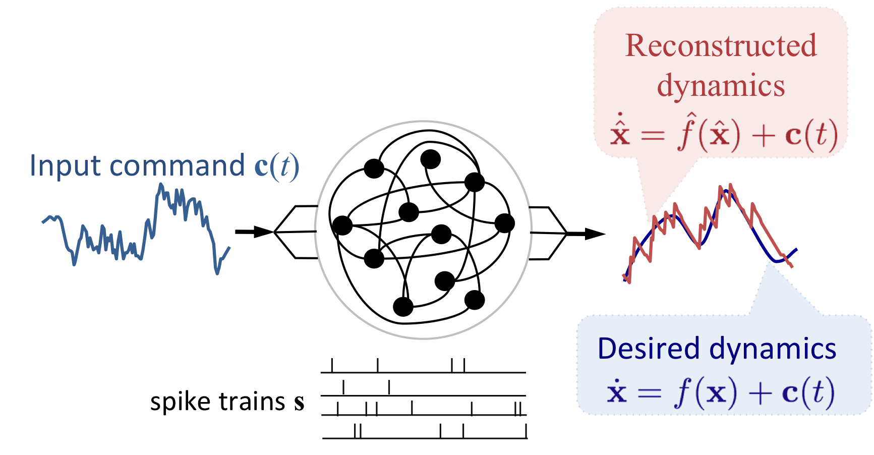
The learning task that we consider is presented in Fig. 1A. An input signal drives a recurrent spiking network. The task is to learn the network connectivity such that a desired dynamics (in blue with the state variable ) can be decoded from the network spike trains (in red with the reconstructed state ). This task could correspond to a sensorimotor learning task, where the network learns a forward internal model that receives the efference copy (i.e. a copy of the input motor command) to predict the body position given the sensory error feedback and the motor command [13].
More formally, we assume that the desired dynamics stem from a ‘‘teacher’’ dynamical system of the general form 11 1 Our dynamic variables and input signals are a function of time but sometimes for simplicity we omit the time variable , writing them as and
| (1) |
in which is a time-dependent dynamic vector of continuous, real-valued variables, is a time-varying input or command signal chosen as a filtered random signal unless otherwise stated, and is an arbitrary, vector-valued function. Note that if the teacher dynamical system is of higher order, we can transform it into a higher-dimensional, first-order dynamical system.
To understand our approach to learning this teacher system, we will first ignore the neural network, and briefly recapitulate how the problem is solved in adaptive nonlinear control theory [4, 5, 12]. Here, the goal is to estimate the parameters of a “student” dynamical system such that its dynamics matches the dynamics of the “teacher” system (See Fig. 1B). The student system has the following form:
| (2) |
where is the dynamic vector variable of the student, is a leak-term, are the parameters of the student dynamics, are the student basis functions (e.g. ), is the tracking error, and is the feedback gain. The goal of learning is to adapt the parameters such that the tracking error is minimized. In the initial phases of learning, the feedback gain is usually set to a large value, which causes the student to follow the desired teaching dynamics closely. In turn, the student variable already traverses the state space correctly which provides the opportunity for adjusting the adaptive parameters in order to learn the dynamics. Once these parameters have been learned (at least approximately), the feedback gain is decreased, which also helps to get good generalization behavior and reduce the number of training iterations. Once the system is learned, the feedback gain can be set to zero, which is what we did in the test phases ().
If the student has sufficiently many rich basis functions to approximate the function , then there exists a solution called . If we define a Lyapunov function as
| (3) |
where is the estimation error and is the matrix trace operator, it can be shown (see Supplementary Materials) that the following adaptation law (or the learning rule)
| (4) |
where is a learning rate, will decrease the Lyapunov function, i.e. . This result together with boundedness conditions for and guarantees that , and hence the tracking error , will asymptotically go to zero and that the system is asymptotically stable [5]. Moreover, if the input is rich enough, then .
3 Learning a functional spiking network

We want to translate our student into a recurrent network of leaky integrate-and-fire (LIF) neurons. Previous work has shown how to implement arbitrary linear or nonlinear dynamical systems in efficient balanced networks [8, 14]. EBN theory is based on two assumptions. First, an estimate of the -dimensional state variable, , can be extracted from the filtered spike trains, , using a linear decoder, such that
| (5) |
where is a fixed decoding weight matrix of size and the relation between and the spike trains is . Second, neurons in the network fire spikes such that this estimate, , closely follows the true state variable, , under cost constraints. Specifically, the network minimizes the following objective function,
| (6) |
where denotes the Lp-norm, is an average over time, and and determine the costs associated with spiking. The first term on the right-hand side of Eq. 6 ensures a good reconstruction, whereas the L2 and L1 cost functions on neural activity ensure a distributed and sparse spiking activity, respectively [8].
The resulting network consists of LIF neurons whose membrane potentials, ’s, obey the equation [8, 15] (see also Supplementary Materials)
| (7) |
and whose firing thresholds are given by , where is the -th column of . The thresholds ensure that each neuron fires only when its spike decreases the objective function (Eq. 6). Differentiating Eq. 7 and simplifying it yields the following membrane potential dynamics
| (8) |
which shows the optimal weight matrix for the fast connections is , where is the identity matrix, and the optimal encoding weight matrix is . In order to implement arbitrary dynamical systems in this framework, we need to include two approximations. First, we can approximate as a sum of the “student” basis functions (similar to Eq. 2), so that , where ’s are the columns of , and can be any sigmoidal nonlinearity set to in the simulations. Second, we can self-consistently replace the state by its estimate based on network activity (Eq. 5). In turn, we obtain (Fig. 2B)
| (9) |
From a biological point-of-view, the last term corresponds to nonlinear and highly structured dendrites. There is evidence that dendrites can perform nonlinear operations [16, 17]. While dendrites are often nonlinear, the required detailed spatial organization of their inputs is rather speculative. To relax this latter constraint, we can take advantage of the fact that the network’s internal state dynamics is extremely robust to large amounts of noise (as ensured by its constant, greedy minimization of its own coding errors), as long as . Thus, we can replace with an unstructured, nonlinear dendrite that receives random connections from other neurons, where ’s are the columns of the matrix . Indeed, the quantity can be written as the sum of its projection onto the decoder , and its projection onto the null space of (denoted by ), so that . Given that EBNs do not control spiking in the null space of the decoder, the second term acts as unstructured noise. 22 2 We note that it would be possible to train the parameters using unsupervised learning, since corresponds to the eigenvectors with non-zero eigenvalues in the neural correlation matrix. This should render the network even more efficient and robust as will be explored in the future.
To clarify the learning problem, we will write the resulting student network dynamics in the general form
| (10) |
We note that the network has three sets of synaptic connections. The feedforward connections, , receive and weight the external signal input, . The fast connections, , guarantee the proper and efficient distribution of spikes across the network. Finally, the slow connections, , implement the dynamics of the student system. In previous work, it is shown how to learn the feedforward connections [18] and the fast recurrent connections [18, 15]. Though all connections could be trained simultaneously, we here concentrate on how to train the slow connections based on example trajectories from an unknown (teacher) dynamical system. We use a fixed random decoding weight matrix (which is close to optimal in the case of uncorrelated command signals) and set the feedforward connections and recurrent connections to their optimal values, and .
A direct translation of the adaptive control to the neural network will finally permit us to define a local learning rule for the slow connections. Rather than feeding back the error into the student network by adding it to its input, we directly inject the errors as feedback to each neuron with connections , which is mathematically equivalent. In the presence of this feedback control loop, the network equation becomes
| (11) |
Moreover is directly related to the coefficients of the basis functions in the control theory framework. This allows us to map the adaptation law (Eq. 4) for the coefficients of the basis function to the following learning rule for the slow connections. Replacing in Eq. 4 with , we obtain
| (12) |
In other words, the resulting learning rule is the product of a pre-synaptic input (passed through the dendritic nonlinearity) and the projection of error feedback. Hence, the learning is local.
For the case of sensorimotor learning, the quantity could correspond to visual or somatosensory “prediction errors”, e.g. the difference between the sensory input and its prediction based on the efference copy of the motor commands. Over the course of learning, the errors become smaller and would eventually vanish in the absence of motor noise or sensory noise. Consequently, the feedback would become silent and could be removed entirely.
The general idea of this derivation, and the mapping from the control-theoretical framework onto efficient balanced networks, is also illustrated in Fig. 2A.


4 Implementing nonlinear dynamics
We employed the framework described above in the following example tasks.
4.1 Bistable attractor
The bistable attractor is an important nonlinear dynamical system which is widely studied in systems neuroscience. We implemented the following one-dimensional attractor dynamics
| (13) |
where is a random input command. This system has two stable fixed-point attractors at and a saddle-point at . We used neurons with random readout weights to implement this system. As shown in Fig. 3A, the random input drives the student network in the beginning of learning. Once this input is zero the desired dynamics given by the teacher (in blue) goes to one of the stable attractors. But the decoded dynamical variable of the network (in red) has not yet learned the desired attractors. After learning (Fig 3B), the network closely follows the desired trajectories in response to a random unseen input (not used during training) and, more importantly, once the input is turned off, it settle on one of the attractors. Note that the network exhibits realistic spiking activity with low firing rates and asynchronous, irregular spiking activity. The overall number of spikes is drastically lower than that of spiking networks that effectively use rate codes [19, 20, 7].
4.2 Motion capture example
We also implemented the walking dynamics from the database of Carnegie Mellon University Motion Capture Library (MOCAP) http://mocap.cs.cmu.edu/. We used a similar preprocessing procedure as in [2]. Briefly, the data was taken from file “08_01.amc” which consisted of 62 channels out of which three were set to zero, converting the movement to a walk on a treadmill. We preprocessed the data by a moving average.
In order to reduce the dimensions of the input signal, we took the first four principle components. This reduced input closely follows the original walking dynamics with minor loss. As the system is a mechanical system, and therefore of second order, we require both velocity and position information. Therefore, in order to be able to model it, we fed both the trajectories and its derivatives to the network, so that the overall input was 8-dimensional. Similarly, we provided a linear combination of the position error and the velocity error as the error feedback to the network. We then learned the dynamics of the 8-dimensional input with two different networks, one of size and and one of size (compare with [2]).
Fig. 4A shows the learned walking, and the left and middle panels of Fig. 4B shows the raster plot of the 50-neuron and 200-neuron networks, respectively. An important feature of our model is its expansion: the number of input channels () must be smaller than the number of neurons () in the network. In order for the network to have the desired aforementioned properties, as a rule of thumb, the expansion ratio () should be larger than 5–10. This expansion provides many possible solutions for the network to perform a task. Thanks to the efficiency principle, the network is able to choose the most efficient one. It should be noted that the realistic spiking activity is closely linked to the expansion: increasing the expansion ratio results in lower firing rate and more irregular spiking activity (compare left and right panels of Fig. 4C). This is one of the main differences with other spiking networks (but in fact they use a rate code) implementing complex dynamics such as the Neural Engineering Framework (NEF) [19, 20], as they would typically need firing rates in the order of the inverse of synaptic time-scales to learn properly. Another striking feature of the model is its robustness to neural death and noise. Thanks to the presence of the fast connections, even if of the neurons in the network are silenced the network would still be able to perform the task with minimal loss in the performance (right-most panel in Fig. 4C). This is consistent with the expected robustness of the EBN framework [21].
5 Discussion
We have proposed a local learning rule in an spiking neural network of LIF neurons for learning arbitrary complex dynamics. The resulting networks exhibit low firing rates with asynchronous, irregular spiking activity where the spiking representation is as efficient as possible. The efficiency principle that we have exploited has direct consequences: the inhibitory input currents in each neuron closely track the excitatory input (E/I balance); and the network is highly robust to noise, neural elimination, and uncertainty in desired dynamics [8, 21]. The learning rule is obtained thanks to concepts and tools in nonlinear adaptive control theory. This approach has the benefit of providing a systematic way to study convergence and stability properties of the learning process which currently is not pursued in the mainstream learning procedures in neuroscience for spiking neurons [2, 22, 14]. Studying the effect of synaptic delays needs to be addressed in future versions of our model, although previous work suggests that increasing the amount of noise may help avoiding oscillation and synchronization [23].
The learning rule can a learn any complex dynamics . However, it may not learn the target dynamics if the input does not have “sufficient richness” condition (see [5]). If function has singularities that make the dynamics unstable, the learning may fail. Another requirement is that the states (for example, position and velocity in the motion capture example) need to be well-defined. Any task that can be cast as a well-behaved dynamical system can be learned in our framework.
The different parts of the spiking network have straightforward biological interpretations. Fast connections could correspond to interneurons which would mostly be driven by monosynaptic, fast AMPA synapses from excitatory neurons, targeting the soma and relying on ionic (GABA-A) neurotransmission. Slow connections could be implemented by slower metabolic channels (e.g. NMDA/GABA-B) and correspond either to direct connections between pyramidal cells, or disynaptic inhibition using another type of interneurons, in the case of negative weights.
The network seems to be highly structured in our framework. However, it has already been shown that most of the other connections in the network can be trained using local spike-time-dependent plasticity rules with the exception of which is the contribution of the present work. In particular, the fast connections can be trained using local plasticity rules, while the feedforward connections (and thus, the decoding weights) can be trained using a Hebbian spike-time-dependent rule [18, 15] . Note that these inhibitory fast connections could be thought of as implementing a kind of ‘dynamic’ Winner-Take-All (WTA) network where once a neuron wins and spikes, then other neurons have a chance to fire as well. This is a different scheme from a distributed WTA of inhibitory neurons [24].
In our general framework, nonlinear dendrites compute the basis functions where we used nonlinearity. However, the learning rule is not limited to that and can work with any basis functions (nonlinearities) that can approximate arbitrary functions e.g. Gaussian, sigmoid basis functions, though sigmoids are more biologically plausible. Apart from the form of nonlinearity, we have a large degree of freedom in the choice of parameters of basis functions i.e., in the design of the dendritic tree. The case that might be easiest to map to the control-theoretic framework is the case where is a low rank matrix. But other cases such as random also work in practice. We provided intuitions for why such a suboptimal architecture still functions: the network activity is forced to be as efficient as possible due to the presence of the fast connections (E/I balance). This defines an optimal combination of neural activities for each state . In other words, neural firing rates become almost completely determined by the internal state estimate (up to their “poisson-like” variability). This neural activity projected onto an arbitrary matrix will also be a function of , plus some unstructured input that may be considered as noise. This noise is automatically compensated by the network robustness. In the case of the walking example, we tested a diagonal matrix (in which case, the dendritic nonlinearity is replaced by a nonlinear transfer function for each neuron) and the network was still able to learn without any difficulty. The best choice of (including the possibility of learning these parameters) remains to be explored further elsewhere. Our approach is aligned with other works taking similar strategies for implementing nonlinearities in recurrent networks [22, 14].
Nonlinear adaptive control theory yields a local learning rule for the Neural Engineering Framework [7] to learn complex dynamics. However, the resulting networks do not implement fast connections to provide spiking efficiency and balance. This in turn implies that they do not scale easily when applied to large dynamics [2, 7], making it more challenging for these networks to exhibit realistic spiking activity and robustness. Our work aims to seamlessly blend nonlinear adaptive control with earlier work on EBNs, which exploits the spiking nature of neural activity rather than treating it as a hindrance.
In conclusion, we argue for a close relationship between spiking efficiency, robustness and the tight E-I balance observed in cortical circuits. We suggest that experimentally observed spike trains, with low-firing rate and asynchronous, irregular spike trains, are a signature of an efficient spike-based coding, and not a noisy rate-based population code. The network effectively implements dimensionality reduction: regardless of its size, the dimensionality of its population dynamics and recurrent weights eventually becomes restricted to the dimensionality of the task, while neural fluctuations occur in direction orthogonal to the task. Thus, we predict that such low-dimensional dynamics emerge through experience in biological neural circuits. Finally, learning in biological circuits would require that feedback connections monitoring the network performance both drive the neurons and modulate learning. Each slow connection is learned as a function of the correlation between presynaptic input rate and postsynaptic error feedback, until this error feedback is canceled. Thus, only neurons with correlations to the error (and presumably contributing to such error) see their synaptic weights change. In contrast, backpropagation would result in diffuse change in the entire network. These predictions have broad implications for Brain Machine Interfaces. In the near future, this theory may pave the way for implementing more complex tasks and for spike based unsupervised, hierarchical and reinforcement learning, in both biological and artificial spiking networks.
The framework presented here can have engineering applications for example in light-weight robots or robots that are sent to space missions where efficiency matters. Furthermore, we have used the framework to estimate the parameters of a desired system but it can also be used for adaptive nonlinear control applications — where the controller needs to adapt to unknown changes in dynamics and kinematics of robots [25, 6] — to give an efficient adaptive spiking controller. The current framework is obtained for deterministic dynamical systems – future work will extend it to stochastic dynamical systems.
References
- [1] P. J. Werbos, “Backpropagation through time: what it does and how to do it,” in Proceedings of the IEEE, 1990.
- [2] D. Sussillo and L. F. Abbott, “Generating Coherent Patterns of Activity from Chaotic Neural Networks,” Neuron, vol. 63, pp. 544–557, Aug. 2009.
- [3] S. B. Laughlin, R. R. de Ruyter van Steveninck, and J. C. Anderson, “The metabolic cost of neural information.,” Nature Neuroscience, vol. 1, pp. 36–41, May 1998.
- [4] J.-J. E. Slotine and J. A. Coetsee, “Adaptive sliding controller synthesis for non-linear systems,” International Journal of Control, vol. 43, pp. 1631–1651, June 1986.
- [5] J.-J. E. Slotine and W. Li, Applied Nonlinear Control. Prentice Hall, 1991.
- [6] T. DeWolf, T. C. Stewart, J.-J. Slotine, and C. Eliasmith, “A spiking neural model of adaptive arm control,” vol. 283, no. 1843, p. 20162134, 2016.
- [7] A. Gilra and W. Gerstner, “Predicting non-linear dynamics: a stable local learning scheme for recurrent spiking neural networks,” arXiv preprint arXiv:1702.06463, 2017.
- [8] M. Boerlin, C. K. Machens, and S. Deneve, “Predictive Coding of Dynamical Variables in Balanced Spiking Networks,” PLoS computational biology, vol. 9, p. e1003258, Nov. 2013.
- [9] S. Deneve and C. K. Machens, “Efficient codes and balanced networks,” Nature Neuroscience, 2016.
- [10] R.-M. Memmesheimer, R. Rubin, B. P. Ölveczky, and H. Sompolinsky, “Learning Precisely Timed Spikes,” Neuron, vol. 82, pp. 925–938, May 2014.
- [11] R. Bourdoukan and S. Deneve, “Enforcing balance allows local supervised learning in spiking recurrent networks,” in Advances in Neural Information Processing Systems (NIPS), pp. 982–990, 2015.
- [12] R. M. Sanner and J.-J. Slotine, “Gaussian networks for direct adaptive control,” IEEE Transactions on neural networks, vol. 3, no. 6, pp. 837–863, 1992.
- [13] D. M. Wolpert and Z. Ghahramani, “Computational principles of movement neuroscience,” Nature Neuroscience, 2000.
- [14] D. Thalmeier, M. Uhlmann, H. J. Kappen, and R.-M. Memmesheimer, “Learning Universal Computations with Spikes.,” PLoS computational biology, vol. 12, p. e1004895, June 2016.
- [15] R. Bourdoukan, D. Barrett, C. K. Machens, and S. Deneve, “Learning optimal spike-based representations,” Advances in Neural Information Processing Systems (NIPS), 2012.
- [16] P. Poirazi, T. Brannon, and B. W. Mel, “Arithmetic of subthreshold synaptic summation in a model CA1 pyramidal cell.,” Neuron, vol. 37, pp. 977–987, Mar. 2003.
- [17] P. Poirazi, T. Brannon, and B. W. Mel, “Pyramidal neuron as two-layer neural network.,” Neuron, vol. 37, pp. 989–999, Mar. 2003.
- [18] W. Brendel, R. Bourdoukan, P. Vertechi, C. K. Machens, and S. Deneve, “Learning to represent signals spike by spike,” arXiv.org:1703.03777, 2017.
- [19] C. Eliasmith and C. H. Anderson, Neural engineering: Computation, representation, and dynamics in neurobiological systems. MIT press, 2004.
- [20] C. Eliasmith, “A unified approach to building and controlling spiking attractor networks,” pp. 1–39, Mar. 2005.
- [21] D. Barrett, S. Deneve, and C. K. Machens, “Optimal compensation for neuron loss,” eLife, vol. 5, p. e12454, 2016.
- [22] L. F. Abbott, B. DePasquale, and R.-M. Memmesheimer, “Building functional networks of spiking model neurons,” Nature Publishing Group, vol. 19, pp. 350–355, Feb. 2016.
- [23] M. Chalk, B. Gutkin, and S. Deneve, “Neural oscillations as a signature of efficient coding in the presence of synaptic delays,” eLife, 2016.
- [24] W. Wang and J.-J. E. Slotine, “Fast computation with neural oscillators,” Neurocomputing, vol. 69, pp. 2320–2326, Oct. 2006.
- [25] C. C. Cheah, C. Liu, and J. Slotine, “Adaptive tracking control for robots with unknown kinematic and dynamic properties,” The International Journal of Robotics Research, vol. 25, pp. 283–296, Mar. 2006.