跳到论文正文
W Papers独立论文阅读器 arXiv:1705.07918 论文正文 计算阅读时间 · 0%
引用这篇论文根据当前论文元数据生成,正式投稿前建议核对。


License: arXiv.org perpetual non-exclusive license
arXiv:1705.07918v1 [quant-ph] 22 May 2017

The Contextual Fraction as a Measure of Contextuality

Samson Abramsky Affiliation: Department of Computer Science, University of Oxford
Wolfson Building, Parks Rd, Oxford OX1 3QD, United Kingdom
   Rui Soares Barbosa Affiliation: Department of Computer Science, University of Oxford
Wolfson Building, Parks Rd, Oxford OX1 3QD, United Kingdom
   Shane Mansfield Affiliation: School of Informatics, University of Edinburgh
Informatics Forum, 10 Crichton Street, Edinburgh EH8 9AB, United Kingdom
   Samson Abramsky Affiliation: Department of Computer Science, University of Oxford
Wolfson Building, Parks Rd, Oxford OX1 3QD, United Kingdom
   Rui Soares Barbosa Affiliation: Department of Computer Science, University of Oxford
Wolfson Building, Parks Rd, Oxford OX1 3QD, United Kingdom
   Shane Mansfield Affiliation: School of Informatics, University of Edinburgh
Informatics Forum, 10 Crichton Street, Edinburgh EH8 9AB, United Kingdom
August 24, 2026
Abstract

We consider the contextual fraction as a quantitative measure of contextuality of empirical models, i.e. tables of probabilities of measurement outcomes in an experimental scenario. It provides a general way to compare the degree of contextuality across measurement scenarios; it bears a precise relationship to violations of Bell inequalities; its value, and a witnessing inequality, can be computed using linear programming; it is monotone with respect to the “free” operations of a resource theory for contextuality; and it measures quantifiable advantages in informatic tasks, such as games and a form of measurement based quantum computing.

pacs
03.65.Ud, 03.67.Mn

Introduction.—

Recent results have established the rôle of contextuality as a resource for increasing the computational power of specific models of computation [1, 2], including enabling universal quantum computation [3]. From this perspective, it is particularly relevant to look for appropriate measures of contextuality, and indeed to pose the question of what constitutes a good measure.

In this Letter, we propose a measure of contextuality—the contextual fraction—which provides a quantitative grading between non-contextuality, at one extreme, and maximal contextuality, at the other. A maximally contextual empirical model is one that admits no proper decomposition into a convex combination of a non-contextual model and another model. In this sense, it is meaningful to consider both the non-contextual and contextual fractions of any no-signalling empirical model.

These definitions are made in the general setting of the approach to contextuality introduced in [4], in which nonlocality is seen as a special case of contextuality.

We show that the contextual fraction has a number of desirable properties: (i) it is fully general in the sense that it applies in any measurement scenario; (ii) it is bounded and normalised, taking values in the interval [0,1][0,1], with 00 indicating non-contextuality and 11 indicating strong contextuality, so it may be used to sensibly compare the degree of contextuality of empirical models not just in a given measurement scenario but also across scenarios; (iii) it has a precise relationship with violations of Bell inequalities, being the maximum normalised violation attained by the empirical model for any Bell inequality on the corresponding measurement scenario; (iv) both the contextual fraction and a witnessing Bell inequality are computable using linear programming—these were implemented and used for computational exploration of some quantum examples; (v) it is monotone with respect to a range of operations on empirical models that intuitively do not generate contextuality, and thus constitute natural “free” operations in a resource theory of contextuality, analogous to the resource theory of entanglement under LOCC operations [5], and subsuming existing resource theories for nonlocality [6, 7, 8]; (vi) finally, it is related to a quantifiable increase of computational power in a certain form of measurement-based quantum computation, sharpening the results of [2], and similarly to advantage in games.

We leave for future work an analysis of the relationship between the contextual fraction and other possible measures 11 1 These include a negative probability measure introduced in [4], contextuality-by-default measures [16], and various other measures considered for nonlocality in specific measurement scenarios, e.g. noise-based [17, 18, 19] and inefficiency-based [20, 21, 22] measures, known to relate to communication complexity [22, 23]., and further development of (vi).

General framework for contextuality.—

We briefly summarise the framework introduced in [4]. The main objects of study are empirical models: tables of data, specifying probability distributions over the joint outcomes of sets of compatible measurements.

A measurement scenario is an abstract description of a particular experimental setup. It consists of a triple ⟨X,ℳ,O⟩\mathopen{\langle}X,\mathcal{M},O\mathclose{\rangle} where: XX is a finite set of measurements; OO is a finite set of outcome values for each measurement; and ℳ\mathcal{M} is a set of subsets of XX. Each C∈ℳC\in\mathcal{M} is called a measurement context, and represents a set of measurements that can be performed together.

Examples of measurement scenarios include multipartite Bell-type scenarios familiar from discussions of nonlocality, Kochen–Specker configurations, measurement scenarios associated with qudit stabiliser quantum mechanics, and more. For example, the well-known (2,2,2)(2,2,2) Bell scenario, where two experimenters, Alice and Bob, can each choose between performing one of two different measurements, say a1a_{1} or a2a_{2} for Alice and b1b_{1} or b2b_{2} for Bob, obtaining one of two possible outcomes, is represented as follows:

X\displaystyle X ={a1,a2,b1,b2}O={0,1}\displaystyle=\mathopen{\{}a_{1},a_{2},b_{1},b_{2}\mathclose{\}}\qquad\qquad O=\mathopen{\{}0,1\mathclose{\}}
ℳ\displaystyle\mathcal{M} ={{a1,b1},{a1,b2},{a2,b1},{a2,b2}}​ .\displaystyle=\mathopen{\{}\mathopen{\{}a_{1},b_{1}\mathclose{\}},\mathopen{\{}a_{1},b_{2}\mathclose{\}},\mathopen{\{}a_{2},b_{1}\mathclose{\}},\mathopen{\{}a_{2},b_{2}\mathclose{\}}\mathclose{\}}\text{ .}

Given this description of the experimental setup, then either performing repeated runs of such experiments with varying choices of measurement context and recording the frequencies of the various outcome events, or calculating theoretical predictions for the probabilities of these outcomes, results in a probability table as in Table 1.

Table 1: Two empirical models on the (2,2,2)(2,2,2) Bell scenario: the well-known CHSH model [9], obtained from local projective measurements equatorial at angles 00 (for a1a_{1}, b1b_{1}) and π/3\nicefrac{{\pi}}{{3}} (for a2a_{2}, b2b_{2}) on the maximally entangled two-qubit Bell-state |Φ+⟩=12​(|00⟩+|11⟩)|\Phi^{+}\rangle=\frac{1}{\sqrt{2}}(|00\rangle+|11\rangle); and the Popescu–Rohrlich box.

AB0 00 11 01 1a1b11/2001/2a1b23/81/81/83/8a2b13/81/81/83/8a2b21/83/83/81/8AB0 00 11 01 1a1b11/2001/2a1b21/2001/2a2b11/2001/2a2b201/21/20\begin{array}[]{cc|cccc}\text{A}&\text{B}&0\,0&0\,1&1\,0&1\,1\\ \hline\cr a_{1}&b_{1}&\nicefrac{{1}}{{2}}&0&0&\nicefrac{{1}}{{2}}\\ a_{1}&b_{2}&\nicefrac{{3}}{{8}}&\nicefrac{{1}}{{8}}&\nicefrac{{1}}{{8}}&\nicefrac{{3}}{{8}}\\ a_{2}&b_{1}&\nicefrac{{3}}{{8}}&\nicefrac{{1}}{{8}}&\nicefrac{{1}}{{8}}&\nicefrac{{3}}{{8}}\\ a_{2}&b_{2}&\nicefrac{{1}}{{8}}&\nicefrac{{3}}{{8}}&\nicefrac{{3}}{{8}}&\nicefrac{{1}}{{8}}\\ \end{array}\quad\quad\begin{array}[]{cc|cccc}\text{A}&\text{B}&0\,0&0\,1&1\,0&1\,1\\ \hline\cr a_{1}&b_{1}&\nicefrac{{1}}{{2}}&0&0&\nicefrac{{1}}{{2}}\\ a_{1}&b_{2}&\nicefrac{{1}}{{2}}&0&0&\nicefrac{{1}}{{2}}\\ a_{2}&b_{1}&\nicefrac{{1}}{{2}}&0&0&\nicefrac{{1}}{{2}}\\ a_{2}&b_{2}&0&\nicefrac{{1}}{{2}}&\nicefrac{{1}}{{2}}&0\\ \end{array}

Such data is formalised as an empirical model for the given measurement scenario ⟨X,ℳ,O⟩\mathopen{\langle}X,\mathcal{M},O\mathclose{\rangle}. For each measurement context CC, there is a probability distribution eCe_{C} on the joint outcomes of performing all the measurements in CC; that is, on the set OCO^{C} of functions assigning an outcome in OO to each measurement in CC.

We require that the marginals of these distributions agree whenever contexts overlap, i.e.

∀C,C′∈ℳ,eC|C∩C′=eC′|C∩C′​ ,\forall{C,C^{\prime}\in\mathcal{M}},\;e_{C}|_{C\cap C^{\prime}}=e_{C^{\prime}}|_{C\cap C^{\prime}}\text{ ,}

where the notation eC|Ue_{C}|_{U} with U⊆CU\subseteq C stands for marginalisation of probability distributions (to ‘forget’ the outcomes of some measurements): for t∈OUt\in O^{U}, eC|U(t):⁣=∑s∈OC,s|U=teC(s)e_{C}|_{U}(t)\mathrel{\mathchoice{\vbox{\hbox{$\displaystyle:$}}}{\vbox{\hbox{$\textstyle:$}}}{\vbox{\hbox{$\scriptstyle:$}}}{\vbox{\hbox{$\scriptscriptstyle:$}}}{=}}\sum_{s\in O^{C},s|_{U}=t}e_{C}(s). The requirement of compatibility of marginals is a generalisation of the usual no-signalling condition, and is satisfied in particular by all empirical models arising from quantum predictions [4].

An empirical model is said to be contextual if this family of distributions cannot itself be obtained as the marginals of a single probability distribution on global assignments of outcomes to all measurements, i.e. a distribution dd on OXO^{X} (where OXO^{X} acts as a canonical set of deterministic hidden variables) such that ∀C∈ℳ,d|C=eC\forall{C\in\mathcal{M}},\;d|_{C}=e_{C}. Equivalently [4], contextual empirical models are those which have no realisation by factorisable hidden variable models; thus for Bell-type measurement scenarios contextuality specialises to the usual notion of nonlocality.

In certain cases, one can witness contextuality from merely the possibilistic, rather than probabilistic, information contained in an empirical model—i.e. which events are possible (with non-zero probability) and which are impossible (with zero probability). A yet stronger form of contextuality occurs when no global assignment of outcomes is even consistent with the possible events: an empirical model ee is said to be strongly contextual if there is no global assignment g∈OXg\in O^{X} such that ∀C∈ℳ,eC​(g|C)>0\forall{C\in\mathcal{M}},\;e_{C}(g|_{C})>0. An example is the Popescu–Rohrlich box (Table 1). This is the highest level in the qualitative hierarchy of strengths of contextuality introduced in [4].

The contextual fraction.—

Given two empirical models ee and e′e^{\prime} on the same measurement scenario and λ∈[0,1]\lambda\in[0,1], we define the empirical model λ​e+(1−λ)​e′\lambda e+(1-\lambda)e^{\prime} by taking the convex sum of probability distributions at each context. Compatibility is preserved by this convex sum, hence it yields a well-defined empirical model.

A natural question to ask is: what fraction of a given empirical model ee admits a non-contextual explanation? This approach enables a refinement of the binary notion of contextuality vs non-contextuality into a quantitative grading. Instead of asking for a probability distribution on global assignments that marginalises to the empirical distributions at each context, we ask only for a subprobability distribution 22 2 A subprobability distribution on a set SS is a map b:S⟶ℝ≥0b:S\longrightarrow\mathbb{R}_{\geq 0} with finite support and w⁡(b)≤1w(b)\leq 1, where w(b):⁣=∑s∈Sb(s)w(b)\mathrel{\mathchoice{\vbox{\hbox{$\displaystyle:$}}}{\vbox{\hbox{$\textstyle:$}}}{\vbox{\hbox{$\scriptstyle:$}}}{\vbox{\hbox{$\scriptscriptstyle:$}}}{=}}\sum_{s\in S}b(s) is called its weight. The set of subprobability distributions on SS is ordered pointwise: b′b^{\prime} is a subdistribution of bb (written b′≤bb^{\prime}\leq b) whenever ∀s∈S,b′​(s)≤b⁡(s)\forall{s\in S},\;b^{\prime}(s)\leq b(s). bb on global assignments OXO^{X} that marginalises at each context to a subdistribution of the empirical data, thus explaining a fraction of the events, i.e. ∀C∈ℳ,b|C≤eC\forall{C\in\mathcal{M}},\;b|_{C}\leq e_{C}. Equivalently, we ask for a convex decomposition

e=λ​eN​C+(1−λ)​e′e=\lambda e^{NC}+(1-\lambda)e^{\prime} (1)

where eN​Ce^{NC} is a non-contextual model and e′e^{\prime} is another (no-signalling) empirical model. The maximum weight of such a global subprobability distribution, or the maximum possible value of λ\lambda in such a decomposition is called the non-contextual fraction of ee, and generalises the local fraction previously introduced for models on Bell-type scenarios [10] 33 3 See also [24, 25] where the term local fraction is actually used.. We denote it by 𝖭𝖢𝖥⁡(e)\mathsf{NCF}(e), and the contextual fraction by 𝖢𝖥(e):⁣=1−𝖭𝖢𝖥(e)\mathsf{CF}(e)\mathrel{\mathchoice{\vbox{\hbox{$\displaystyle:$}}}{\vbox{\hbox{$\textstyle:$}}}{\vbox{\hbox{$\scriptstyle:$}}}{\vbox{\hbox{$\scriptscriptstyle:$}}}{=}}1-\mathsf{NCF}(e).

The notion of contextual fraction in general scenarios was introduced in [4], where it was proved that a model is strongly contextual if and only if its contextual fraction is 11. In fact, in any convex decomposition of the form (1) giving maximal weight to the non-contextual model, the other model will necessarily be strongly contextual. This means that any empirical model ee admits a convex decomposition

e=𝖭𝖢𝖥⁡(e)​eN​C+𝖢𝖥⁡(e)​eS​Ce=\mathsf{NCF}(e)\,e^{NC}+\mathsf{CF}(e)\,e^{SC} (2)

into a non-contextual and a strongly contextual model. Note that eN​Ce^{NC} and eS​Ce^{SC} are not necessarily unique.

Computing the contextual fraction via LP.—

The task of finding a consistent probability subdistribution with maximum weight for a given empirical model can be formulated as a linear programming problem. This is a relaxation of the test for contextuality by solving a system of linear equations over the nonnegative reals from [4].

Fix a measurement scenario ⟨X,ℳ,O⟩\mathopen{\langle}X,\mathcal{M},O\mathclose{\rangle}. Let n:⁣=|OX|n\mathrel{\mathchoice{\vbox{\hbox{$\displaystyle:$}}}{\vbox{\hbox{$\textstyle:$}}}{\vbox{\hbox{$\scriptstyle:$}}}{\vbox{\hbox{$\scriptscriptstyle:$}}}{=}}|O^{X}| be the number of global assignments gg, and m:⁣=∑C∈ℳ|OC|=|{⟨C,s⟩∣C∈ℳ,s∈OC}|m\mathrel{\mathchoice{\vbox{\hbox{$\displaystyle:$}}}{\vbox{\hbox{$\textstyle:$}}}{\vbox{\hbox{$\scriptstyle:$}}}{\vbox{\hbox{$\scriptscriptstyle:$}}}{=}}\sum_{C\in\mathcal{M}}|O^{C}|=|\left\{\mathopen{\langle}C,s\mathclose{\rangle}\mid C\in\mathcal{M},s\in O^{C}\right\}| be the number of local assignments ranging over contexts. The incidence matrix [4] 𝐌\mathbf{M} is an m×nm\times n (0,1)(0,1)-matrix that records the restriction relation between global and local assignments:

𝐌[⟨C,s⟩,g]:⁣={1​ if g|C=s;0​ otherwise.\mathbf{M}[\mathopen{\langle}C,s\mathclose{\rangle},g]\mathrel{\mathchoice{\vbox{\hbox{$\displaystyle:$}}}{\vbox{\hbox{$\textstyle:$}}}{\vbox{\hbox{$\scriptstyle:$}}}{\vbox{\hbox{$\scriptscriptstyle:$}}}{=}}\begin{cases}1\;\text{ if $g|_{C}=s$;}\\ 0\;\text{ otherwise.}\end{cases}

An empirical model ee can be represented as a vector 𝐯e∈ℝm\mathbf{v}^{e}\in\mathbb{R}^{m}, with the component 𝐯e​[⟨C,s⟩]\mathbf{v}^{e}[\mathopen{\langle}C,s\mathclose{\rangle}] recording the probability given by the model to the assignment ss at the measurement context CC, eC​(s)e_{C}(s). This vector is a flattened version of the table used to represent the empirical model (e.g. Table 1). The columns of the incidence matrix, 𝐌⁡[−,g]\mathbf{M}[-,g], are the vectors corresponding to the (non-contextual) deterministic models obtained from global assignments g∈OXg\in O^{X}. Recall that every non-contextual model can be written as a mixture of these. A probability distribution on global assignments can be represented as a vector 𝐝∈ℝn\mathbf{d}\in\mathbb{R}^{n} with non-negative components summing to 11, and then the corresponding non-contextual model is represented by the vector 𝐌​𝐝\mathbf{M}\,\mathbf{d}. So a model ee is non-contextual if and only if there exists a 𝐝∈ℝn\mathbf{d}\in\mathbb{R}^{n} such that:

𝐌​𝐝=𝐯e and 𝐝≥𝟎​ .\mathbf{M}\,\mathbf{d}\,=\,\mathbf{v}^{e}\quad\quad\text{ and }\quad\quad\mathbf{d}\geq\mathbf{0}\text{ .}

Note that the first condition implies that 𝐝\mathbf{d} is normalised.

A global subprobability distribution is also represented by a vector 𝐛∈ℝn\mathbf{b}\in\mathbb{R}^{n} with non-negative components, its weight being given by the dot product 𝟏⋅𝐛\mathbf{1}\cdot\mathbf{b}, where 𝟏∈ℝn\mathbf{1}\in\mathbb{R}^{n} is the vector whose nn components are each 11. The following LP thus calculates the non-contextual fraction of an empirical model ee, with 𝖭𝖢𝖥⁡(e)=𝟏⋅𝐛∗\mathsf{NCF}(e)=\mathbf{1}\cdot\mathbf{b}^{*} where 𝐛∗\mathbf{b}^{*} is an optimal solution:

Find \displaystyle\texttt{Find }\;\; 𝐛∈ℝn\displaystyle\mathbf{b}\in\mathbb{R}^{n} (3)
maximising \displaystyle\texttt{maximising }\;\; 𝟏⋅𝐛\displaystyle\mathbf{1}\cdot\mathbf{b}
subject to \displaystyle\texttt{subject to }\;\; 𝐌​𝐛≤𝐯e\displaystyle\mathbf{M}\,\mathbf{b}\,\leq\,\mathbf{v}^{e}
and \displaystyle\texttt{and }\;\; 𝐛≥ 0\displaystyle\mathbf{b}\,\geq\,\mathbf{0} .\displaystyle\text{ .}

Violations of generalised Bell inequalities.—

We now provide further justification for viewing the contextual fraction as a measure of contextuality by relating it to violations of contextuality-witnessing inequalities.

An inequality for a scenario ⟨X,ℳ,O⟩\mathopen{\langle}X,\mathcal{M},O\mathclose{\rangle} is given by a vector 𝐚∈ℝm\mathbf{a}\in\mathbb{R}^{m} of real coefficients indexed by local assignments ⟨C,s⟩\mathopen{\langle}C,s\mathclose{\rangle}, and a bound RR. For a model ee, the inequality reads 𝐚⋅𝐯e≤R\mathbf{a}\cdot\mathbf{v}^{e}\,\leq\,R, where

𝐚⋅𝐯e=∑C∈ℳ,s∈OC𝐚⁡[⟨C,s⟩]​eC​(s)​ .\mathbf{a}\cdot\mathbf{v}^{e}\;=\;\sum_{C\in\mathcal{M},s\in O^{C}}\,\mathbf{a}[\mathopen{\langle}C,s\mathclose{\rangle}]\,e_{C}(s)\text{ .}

Without loss of generality, we can take RR to be non-negative (in fact, even R=0R=0) as any inequality is equivalent to one of this form. We call it a Bell inequality if it is satisfied by every non-contextual model. This generalises the usual notion of Bell inequality, which is defined for Bell-type scenarios for nonlocality, to apply to any contextuality scenario. If, moreover, it is saturated by some non-contextual model, the Bell inequality is said to be tight. A Bell inequality establishes a bound for the value of 𝐚⋅𝐯e\mathbf{a}\cdot\mathbf{v}^{e} amongst non-contextual models ee. For more general models, this quantity is limited only by the algebraic bound

∥𝐚∥:⁣=∑C∈ℳmax{𝐚[⟨C,s⟩]∣s∈OC} .\|\mathbf{a}\|\mathrel{\mathchoice{\vbox{\hbox{$\displaystyle:$}}}{\vbox{\hbox{$\textstyle:$}}}{\vbox{\hbox{$\scriptstyle:$}}}{\vbox{\hbox{$\scriptscriptstyle:$}}}{=}}\sum_{C\in\mathcal{M}}\max\left\{\mathbf{a}[\mathopen{\langle}C,s\mathclose{\rangle}]\mid s\in O^{C}\right\}\text{ .}

Note that we will consider only inequalities satisfying R<‖𝐚‖R<\|\mathbf{a}\|, which excludes inequalities trivially satisfied by all models, and avoids cluttering the presentation with special caveats about division by 0.

The violation of a Bell inequality ⟨𝐚,R⟩\mathopen{\langle}\mathbf{a},R\mathclose{\rangle} by a model ee is max⁡{0,𝐚⋅𝐯e−R}\max\mathopen{\{}0,\mathbf{a}\cdot\mathbf{v}^{e}-R\mathclose{\}}. However, it is useful to normalise this value by the maximum possible violation in order to give a better idea of the extent to which the model violates the inequality. The normalised violation of the Bell inequality by the model ee is

max⁡{0,𝐚⋅𝐯e−R}‖𝐚‖−R​ .\frac{\max\mathopen{\{}0,\mathbf{a}\cdot\mathbf{v}^{e}-R\mathclose{\}}}{\|\mathbf{a}\|-R}\text{ .}
Theorem 1.

Let ee be an empirical model. (i) The normalised violation by ee of any Bell inequality is at most 𝖢𝖥⁡(e)\mathsf{CF}(e); (ii) if 𝖢𝖥⁡(e)>0\mathsf{CF}(e)>0, this bound is attained, i.e. there exists a Bell inequality whose normalised violation by ee is 𝖢𝖥⁡(e)\mathsf{CF}(e); (iii) moreover, for any decomposition of the form (2), this Bell inequality is tight at the non-contextual model eN​Ce^{NC} (provided 𝖭𝖢𝖥⁡(e)>0\mathsf{NCF}(e)>0) and maximally violated at the strongly contextual model eS​Ce^{SC}.

The proof of this result is based on the Strong Duality theorem of linear programming [11]. It provides an LP method of calculating a witnessing Bell inequality for any empirical model ee. The symmetric dual of (3) is the following LP:

Find \displaystyle\texttt{Find }\;\; 𝐲∈ℝm\displaystyle\mathbf{y}\in\mathbb{R}^{m} (4)
minimising \displaystyle\texttt{minimising }\;\; 𝐲⋅𝐯e\displaystyle\mathbf{y}\cdot\mathbf{v}^{e}
subject to \displaystyle\texttt{subject to }\;\; 𝐌T​𝐲≥ 1\displaystyle\mathbf{M}^{T}\,\mathbf{y}\,\geq\,\mathbf{1}
and \displaystyle\texttt{and }\;\; 𝐲≥ 0\displaystyle\mathbf{y}\,\geq\,\mathbf{0} .\displaystyle\text{ .}

The Strong Duality theorem says that, if 𝐛∗\mathbf{b}^{*} is a solution for (3), then there is a solution 𝐲∗\mathbf{y}^{*} for (4) satisfying

𝟏⋅𝐛∗=𝐲∗⋅𝐯e.\mathbf{1}\cdot\mathbf{b}^{*}\;=\;\mathbf{y}^{*}\cdot\mathbf{v}^{e}. (5)

Defining 𝐚∗:⁣=|ℳ|−1𝟏−𝐲∗\mathbf{a}^{*}\mathrel{\mathchoice{\vbox{\hbox{$\displaystyle:$}}}{\vbox{\hbox{$\textstyle:$}}}{\vbox{\hbox{$\scriptstyle:$}}}{\vbox{\hbox{$\scriptscriptstyle:$}}}{=}}|\mathcal{M}|^{\raisebox{0.60275pt}{$\scriptscriptstyle-1$}}\mathbf{1}-\mathbf{y}^{*}, one can show using (5) that the Bell inequality determined by 𝐚∗\mathbf{a}^{*} as the vector of coefficients and with bound R=0R=0 satisfies parts (ii) and (iii) of the Theorem. A detailed proof is provided in the supplemental material 44 4 See Supplemental Material at [URL will be inserted by publisher] for rigorous proofs and further details on our computational explorations..

Monotonicity.—

A key desideratum of a useful measure of contextuality is that it be a monotone for the free operations of a resource theory for contextuality. A fuller treatment of this subject will be presented in a forthcoming article by the authors; here, we consider the properties of the contextual fraction with respect to some of these operations.

We consider the following operations: first, translation of measurements (including restriction to a smaller set of measurements, replication of measurements, etc.); secondly, coarse-graining of outcomes. Special cases of these give isomorphic relabelling of measurements and outcomes. We also consider operations that combine two empirical models to build a new one. The first of these is probabilistic mixing with a weight λ∈[0,1]\lambda\in[0,1]. The second is controlled choice: given empirical models ee and e′e^{\prime} on scenarios ⟨X,ℳ,O⟩\mathopen{\langle}X,\mathcal{M},O\mathclose{\rangle} and ⟨X′,ℳ′,O⟩\mathopen{\langle}X^{\prime},\mathcal{M}^{\prime},O\mathclose{\rangle} respectively, e&e′e\mathbin{\&}e^{\prime} is defined on the scenario ⟨X⊔X′,ℳ⊔ℳ′,O⟩\mathopen{\langle}X\sqcup X^{\prime},\mathcal{M}\sqcup\mathcal{M}^{\prime},O\mathclose{\rangle} by (e&e′)C:=eC(e\mathbin{\&}e^{\prime})_{C}:=e_{C} for C∈ℳC\in\mathcal{M} and (e&e′)C′:=eC′(e\mathbin{\&}e^{\prime})_{C^{\prime}}:=e_{C^{\prime}} for C′∈ℳ′C^{\prime}\in\mathcal{M}^{\prime}. The third is a product: e⊗e′e\otimes e^{\prime} is an empirical model defined on the scenario ⟨X⊔X′,ℳ⋆ℳ′,O⟩\mathopen{\langle}X\sqcup X^{\prime},\mathcal{M}\star\mathcal{M}^{\prime},O\mathclose{\rangle}, where ℳ⋆ℳ′:={C⊔C′∣C∈ℳ,C′∈ℳ′}\mathcal{M}\star\mathcal{M}^{\prime}:=\left\{C\sqcup C^{\prime}\mid C\in\mathcal{M},C^{\prime}\in\mathcal{M}^{\prime}\right\}, by (e⊗e′)C⊔C′​⟨s,s′⟩:=eC​(s)​eC′′​(s′)(e\otimes e^{\prime})_{C\sqcup C^{\prime}}\mathopen{\langle}s,s^{\prime}\mathclose{\rangle}:=e_{C}(s)\,e^{\prime}_{C^{\prime}}(s^{\prime}) for all C∈MC\in M, C′∈ℳ′C^{\prime}\in\mathcal{M}^{\prime}, s∈OCs\in O^{C}, and s′∈OC′s^{\prime}\in O^{C^{\prime}}.

These operations can be used to construct any local empirical model on Bell scenarios starting from a very simple “generator”: a deterministic model over a single measurement. This is illustrated in the supplemental material.

Theorem 2.

The contextual fraction is invariant under relabellings, and non-increasing under translation of measurements and coarse-graining of outcomes. For the combining operations, it satisfies the following properties:

  • •

    𝖢𝖥⁡(λ​e+(1−λ)​e′)≤λ​𝖢𝖥​(e)+(1−λ)​𝖢𝖥​(e)\mathsf{CF}(\lambda e+(1-\lambda)e^{\prime})\leq\lambda\mathsf{CF}(e)+(1-\lambda)\mathsf{CF}(e)

  • •

    𝖢𝖥⁡(e&e′)=max⁡{𝖢𝖥⁡(e),𝖢𝖥⁡(e′)}\mathsf{CF}(e\mathbin{\&}e^{\prime})=\max\mathopen{\{}\mathsf{CF}(e),\mathsf{CF}(e^{\prime})\mathclose{\}}

  • •

    𝖢𝖥⁡(e⊗e′)=𝖢𝖥⁡(e)+𝖢𝖥⁡(e′)−𝖢𝖥⁡(e)​𝖢𝖥​(e′)\mathsf{CF}(e\otimes e^{\prime})=\mathsf{CF}(e)+\mathsf{CF}(e^{\prime})-\mathsf{CF}(e)\mathsf{CF}(e^{\prime})

A consequence of this result is that, for any of the combining operations, when e′e^{\prime} is a non-contextual model (and thus composing with e′e^{\prime} is a free operation), 𝖢𝖥\mathsf{CF} acts as a monotone: the contextual fraction of the new model is at most that of ee (in fact, with equality holding for both choice and product).

Computational explorations.—

General computational tools in the form of a Mathematica package have been developed implementing the two LPs described above to calculate, for any empirical model in any scenario: the (non-)contextual fraction, a decomposition of the form (2), and the generalised Bell inequality from Theorem 1-(ii) for which the maximal violation is achieved. The package also calculates quantum empirical models from any (pure or mixed) state and any specified sets of compatible measurements.

As an example to illustrate the use of this package, we consider the empirical models obtained from local measurements on various nn-qubit states. On each qubit, we allow the same two local measurements, equatorial on the Bloch sphere, parametrised by angles ϕ1\phi_{1} and ϕ2\phi_{2}. Figure 1 plots the contextual fraction of the resulting models as a function of these angles.
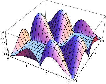
Refer to caption Refer to caption Refer to caption
(a) (b) (c)
Figure 1: Plots of the contextual fraction for empirical models obtained with projective measurements at ϕ1\phi_{1} and ϕ2\phi_{2} in the XX–YY plane for each qubit on the states: (a) the Bell state |Φ+⟩:⁣=|00⟩+|11⟩2|\Phi^{+}\rangle\mathrel{\mathchoice{\vbox{\hbox{$\displaystyle:$}}}{\vbox{\hbox{$\textstyle:$}}}{\vbox{\hbox{$\scriptstyle:$}}}{\vbox{\hbox{$\scriptscriptstyle:$}}}{=}}\frac{|00\rangle+|11\rangle}{\sqrt{2}}; (b) |ψ𝖦𝖧𝖹⁡(3)⟩|\psi_{\mathsf{GHZ}(3)}\rangle; (c) |ψ𝖦𝖧𝖹⁡(4)⟩|\psi_{\mathsf{GHZ}(4)}\rangle, where the nn-partite GHZ state (n>2n>2) is given by |ψ𝖦𝖧𝖹⁡(n)⟩=|0⟩⊗n+|1⟩⊗n2|\psi_{\mathsf{GHZ}(n)}\rangle=\frac{|0\rangle^{\otimes n}+|1\rangle^{\otimes n}}{\sqrt{2}}.

Computational explorations of this kind can be a useful tool for guiding research, pointing the way to conjectures and results (e.g. [12, 13, 14]). A more detailed analysis of the examples from Figure 1, leading to the characterisation of a family of strongly contextual models arising from nn-partite GHZ states, can be found in the supplemental material.

Applications to quantum computation.—

Contextuality has been associated with quantum advantage in certain information-processing and computational tasks. One use for a measure of contextuality is to quantify such advantages.

One computational model in which contextuality has been associated with an advantage is measurement-based quantum computation (MBQC). An l​2l2-MBQC is a process with mm classical bits of input and ll of output, using an (n,2,2)(n,2,2) empirical model (nn parties, 22 measurement settings per party, 22 outcomes per measurement) as a resource. The classical control—which pre-processes the inputs, determines the flow of measurements by choosing which sites to measure next and with which measurement setting (potentially depending on previous outcomes), and post-processes to produce the outputs—can only perform ℤ2\mathbb{Z}_{2}-linear computations. The additional power to compute non-linear functions thus resides in certain resource empirical models.

In [2, Theorem 2] it was shown that if an l​2l2-MBQC process deterministically calculates a non-ℤ2\mathbb{Z}_{2}-linear Boolean function f:2m⟶2lf:2^{m}\longrightarrow 2^{l}, then the resource is necessarily strongly contextual. A probabilistic version was also obtained in [2, Theorem 3]: contextuality must be present whenever a non-linear function is calculated with a sufficiently large probability of success. By analysing that proof, we extract a sharpened version of this result establishing a precise relationship between the hardness (non-linearity) of the function, the probability of success, and the contextual fraction.

The average distance between two Boolean functions f,g:2m⟶2lf,g:2^{m}\longrightarrow 2^{l} is given by d~(f,g):⁣=2−m|{𝐢∈2m∣f(𝐢)≠g(𝐢)}|\tilde{d}(f,g)\mathrel{\mathchoice{\vbox{\hbox{$\displaystyle:$}}}{\vbox{\hbox{$\textstyle:$}}}{\vbox{\hbox{$\scriptstyle:$}}}{\vbox{\hbox{$\scriptscriptstyle:$}}}{=}}2^{-m}|\left\{\mathbf{i}\in 2^{m}\mid f(\mathbf{i})\neq g(\mathbf{i})\right\}|. The average distance of ff to the closest ℤ2\mathbb{Z}_{2}-linear function is denoted by ν~​(f)\tilde{\nu}(f).

Theorem 3.

Let f:2m⟶2lf:2^{m}\longrightarrow 2^{l} be a Boolean function and consider an l​2l2-MBQC that uses the empirical model ee to compute ff with average success probability p¯S\bar{p}_{S} over all 2m2^{m} possible inputs, and corresponding average failure probability p¯F=1−p¯S\bar{p}_{F}=1-\bar{p}_{S}. Then, p¯F≥𝖭𝖢𝖥⁡(e)​ν~​(f)\bar{p}_{F}\;\geq\;\mathsf{NCF}(e)\tilde{\nu}(f).

Note that for deterministic computation (p¯S=1\bar{p}_{S}=1) of a non-linear function (ν~>0\tilde{\nu}>0), we require strong contextuality (𝖭𝖢𝖥⁡(e)=0\mathsf{NCF}(e)=0), recovering the deterministic result in [2]. More generally, for a given non-linear function, the higher the desired success probability the larger the contextual fraction must be. Additional details, including a rigorous presentation and proof, may be found in the supplemental material.

Similar results can be obtained to quantify advantage in games, generalizing XOR games on Bell scenarios. A game is specified by nn boolean formulae, one for each context, which describe the winning condition that the output must satisfy. If the formulae are kk-consistent, meaning that at most kk of them have a joint satisfying assignment, then the hardness of the game is measured by (n−k)n\frac{(n-k)}{n}. One can show that p¯F≥𝖭𝖢𝖥⁡(e)​(n−k)n\bar{p}_{F}\geq\mathsf{NCF}(e)\frac{(n-k)}{n}, relating the probability of success, the non-contextual fraction, and the hardness of the task. See [15] for the relation with Bell inequalities, from which a proof of this result follows. Details are given in the supplemental material, Theorem 4. Further development of these ideas is a topic for future research.

Acknowledgements.—

This work was done in part while the authors visited the Simons Institute for the Theory of Computing (supported by the Simons Foundation) at the University of California, Berkeley, as participants of the Logical Structures in Computation programme, and while SM was based at l’Institut de Recherche en Informatique Fondamentale, Université Paris Diderot – Paris 7. Support from the following is also gratefully acknowledged: EPSRC EP/N018745/1, Contextuality as a Resource in Quantum Computation (SA, RSB); Fondation Sciences Mathématiques de Paris, postdoctoral research grant eotpFIELD15RPOMT-FSMP1, Contextual Semantics for Quantum Theory (SM); the Oxford Martin School James Martin Program on Bio-inspired Quantum Technologies, (SA, SM, RSB); FCT – Fundação para a Ciência e Tecnologia (Portuguese Foundation for Science and Technology), PhD grant SFRH/BD/94945/2013 (RSB).

References

  • [1] J. Anders and D. E. Browne, Phys. Rev. Lett. 102, 050502 (2009).
  • [2] R. Raussendorf, Phys. Rev. A 88, 022322 (2013).
  • [3] M. Howard, J. Wallman, V. Veitch, and J. Emerson, Nature 510, 351 (2014).
  • [4] S. Abramsky and A. Brandenburger, New J. Phys. 13, 113036 (2011).
  • [5] R. Horodecki, P. Horodecki, M. Horodecki, and K. Horodecki, Rev. Mod. Phys. 81, 865 (2009).
  • [6] J. Barrett, N. Linden, S. Massar, S. Pironio, S. Popescu, and D. Roberts, Physical Review A 71, 022101 (2005).
  • [7] R. Gallego, L. E. Würflinger, A. Acín, and M. Navascués, Physical Review Letters 109, 070401 (2012).
  • [8] J. I. de Vicente, J. Phys. A: Math. Theor. 47, 424017 (2014).
  • [9] J. F. Clauser, M. A. Horne, A. Shimony, and R. A. Holt, Phys. Rev. Lett. 23, 880 (1969).
  • [10] A. C. Elitzur, S. Popescu, and D. Rohrlich, Phys. Lett. A 162, 25 (1992).
  • [11] G. B. Dantzig and M. N. Thapa, Linear programming 2, Springer Series in Operations Research and Financial Engineering (Springer Verlag, 2003).
  • [12] S. Abramsky, C. M. Constantin, and S. Ying, Information and Computation 250, 3 (2016).
  • [13] S. Abramsky and C. Constantin, Electronic Proceedings in Theoretical Computer Science 171, 10 (2014).
  • [14] S. Mansfield, DPhil thesis, University of Oxford (2013).
  • [15] S. Abramsky and L. Hardy, Physical Review A 85, 062114 (2012).
  • [16] E. N. Dzhafarov, J. V. Kujala, and V. H. Cervantes, in International Symposium on Quantum Interaction (Springer, 2015), pp. 12–23.
  • [17] D. Kaszlikowski, P. Gnaciński, M. Żukowski, W. Miklaszewski, and A. Zeilinger, Physical Review Letters 85, 4418 (2000).
  • [18] A. Acín, T. Durt, N. Gisin, and J. I. Latorre, Physical Review A 65, 052325 (2002).
  • [19] M. Junge, C. Palazuelos, D. Pérez-García, I. Villanueva, and M. M. Wolf, Physical review letters 104, 170405 (2010).
  • [20] S. Massar, S. Pironio, J. Roland, and B. Gisin, Physical Review A 66, 052112 (2002).
  • [21] S. Laplante, V. Lerays, and J. Roland, in International Colloquium on Automata, Languages, and Programming (Springer, 2012), pp. 617–628.
  • [22] J. Degorre, M. Kaplan, S. Laplante, and J. Roland, in International Symposium on Mathematical Foundations of Computer Science (Springer, 2009), pp. 270–281.
  • [23] S. Laplante, M. Laurière, A. Nolin, J. Roland, and G. Senno, in 11th Conference on the Theory of Quantum Computation, Communication and Cryptography (2016).
  • [24] J. Barrett, A. Kent, and S. Pironio, Phys. Rev. Lett. 97, 170409 (2006).
  • [25] L. Aolita, R. Gallego, A. Acín, A. Chiuri, G. Vallone, P. Mataloni, and A. Cabello, Phys. Rev. A 85, 032107 (2012).
  • [26] D. M. Greenberger, M. A. Horne, and A. Zeilinger, in Bell’s theorem, quantum theory, and conceptions of the universe, edited by M. Kafatos (Kluwer, 1989), pp. 69–72.
  • [27] N. D. Mermin, Physical Review Letters 65, 1838 (1990).
  • [28] S. Abramsky, S. Mansfield, and R. S. Barbosa, in Proceedings 8th International Workshop on Quantum Physics and Logic, Nijmegen, Netherlands, October 27–29, 2011, edited by B. Jacobs, P. Selinger, and B. Spitters (Open Publishing Association, 2012), vol. 95 of Electronic Proceedings in Theoretical Computer Science, pp. 1–14.
  • [29] R. Cleve and R. Mittal, in Automata, Languages, and Programming, ICALP 2014, edited by J. Esparza, P. Fraigniaud, T. Husfeldt, and E. Koutsoupias (Springer, 2014), vol. 8572 of Lecture Notes in Computer Science, pp. 320–331.
  • [30] R. Cleve, L. Liu, and W. Slofstra, Journal of Mathematical Physics 58, 012202 (2017).
  • [31] L. Mančinska and D. E. Roberson, Journal of Combinatorial Theory, Series B 118, 228 (2016).
  • [32] S. Abramsky, R. S. Barbosa, N. de Silva, and O. Zapata, The quantum monad on relational structures, Submitted for publication (2017).

The Contextual Fraction as a Measure of Contextuality—Supplemental Material August 24, 2026

Appendix A A. Contextual fraction and violations of Bell inequalities (Proof of Theorem 1)

Theorem 1 establishes the close link between the contextual fraction of an empirical model and the violation of generalised Bell inequalities by that model. In the main text, we presented this result along with the broad idea of its proof, with particular emphasis on the linear program that calculates the Bell inequality for which a given model achieves a maximal violation. For completeness, we include here the detailed proof of the three statements.

As a preliminary remark, we note that the Strong Duality theorem of Linear Programming does indeed apply here, since the set of feasible solutions is bounded and non-empty. Indeed, non-emptiness holds since the zero vector is feasible, while boundedness holds since the constraints imply that every component of a vector satisfying them must lie in the unit interval.

See 1

Proof.

(i) This follows from the decomposition of ee into a non-contextual and a strongly contextual models,

e=𝖭𝖢𝖥⁡(e)​eN​C+𝖢𝖥⁡(e)​eS​C​ .e=\mathsf{NCF}(e)e^{NC}+\mathsf{CF}(e)e^{SC}\text{ .}

For any Bell inequality, determined by ⟨𝐚,R⟩\mathopen{\langle}\mathbf{a},R\mathclose{\rangle}, with ‖𝐚‖>R\|\mathbf{a}\|>R, the left-hand side of the inequality for the model ee adds up to

𝐚⋅𝐯e\displaystyle\mathbf{a}\cdot\mathbf{v}^{e}
=\displaystyle=  ​{ by decomposition above and linearity of (𝐚⋅−) }\displaystyle\rule{20.00003pt}{0.0pt}\{\mbox{\rule[-6.99997pt]{0.0pt}{18.00005pt} \footnotesize by decomposition above and linearity of $(\mathbf{a}\cdot{-})$ \/}\}
𝖭𝖢𝖥⁡(e)​𝐚⋅𝐯eN​C+𝖢𝖥⁡(e)​𝐚⋅𝐯eS​C\displaystyle\mathsf{NCF}(e)\,\mathbf{a}\cdot\mathbf{v}^{e^{NC}}\;+\;\mathsf{CF}(e)\,\mathbf{a}\cdot\mathbf{v}^{e^{SC}}
≤\displaystyle\leq  ​{ since 𝐚⋅𝐯eN​C≤R and 𝐚⋅𝐯eS​C≤‖𝐚‖ }\displaystyle\rule{20.00003pt}{0.0pt}\{\mbox{\rule[-6.99997pt]{0.0pt}{18.00005pt} \footnotesize since $\mathbf{a}\cdot\mathbf{v}^{e^{NC}}\leq R$ and $\mathbf{a}\cdot\mathbf{v}^{e^{SC}}\leq\|\mathbf{a}\|$ \/}\}
𝖭𝖢𝖥⁡(e)​R+𝖢𝖥⁡(e)​‖𝐚‖\displaystyle\mathsf{NCF}(e)\,R\;+\;\mathsf{CF}(e)\,\|\mathbf{a}\|
=\displaystyle=
𝖭𝖢𝖥⁡(e)​R+𝖢𝖥⁡(e)​R+𝖢𝖥⁡(e)​(‖𝐚‖−R)\displaystyle\mathsf{NCF}(e)\,R\;+\;\mathsf{CF}(e)\,R\;+\;\mathsf{CF}(e)\,(\|\mathbf{a}\|-R)
=\displaystyle=  ​{ by 𝖭𝖢𝖥⁡(e)+𝖢𝖥⁡(e)=1 }\displaystyle\rule{20.00003pt}{0.0pt}\{\mbox{\rule[-6.99997pt]{0.0pt}{18.00005pt} \footnotesize by $\mathsf{NCF}(e)+\mathsf{CF}(e)=1$ \/}\}
R+𝖢𝖥​(e)​(‖𝐚‖−R)​ .\displaystyle R\;+\;\mathsf{CF}(e)\,(\|\mathbf{a}\|-R)\text{ .}

Therefore, since ‖𝐚‖>R\|\mathbf{a}\|>R, we have, as required,

𝐚⋅𝐯e−R‖𝐚‖−R≤𝖢𝖥⁡(e)​ .\frac{\mathbf{a}\cdot\mathbf{v}^{e}-R}{\|\mathbf{a}\|-R}\;\leq\;\mathsf{CF}(e)\text{ .}

(ii) Recall the LP (3) that yields the (non-)contextual fraction of a model ee. Its symmetric dual is the following:

Find \displaystyle\texttt{Find }\;\; 𝐲∈ℝm\displaystyle\mathbf{y}\in\mathbb{R}^{m}
minimising \displaystyle\texttt{minimising }\;\; 𝐯e⋅𝐲\displaystyle\mathbf{v}^{e}\cdot\mathbf{y}
subject to \displaystyle\texttt{subject to }\;\; 𝐌⊺​𝐲≥ 1\displaystyle\mathbf{M}^{\intercal}\,\mathbf{y}\,\geq\,\mathbf{1}
and \displaystyle\texttt{and }\;\; 𝐲≥ 0\displaystyle\mathbf{y}\,\geq\,\mathbf{0} .\displaystyle\text{ .}

Under the transformation of variables

𝐚:⁣=|ℳ|−1𝟏−𝐲 ,\mathbf{a}\;\mathrel{\mathchoice{\vbox{\hbox{$\displaystyle:$}}}{\vbox{\hbox{$\textstyle:$}}}{\vbox{\hbox{$\scriptstyle:$}}}{\vbox{\hbox{$\scriptscriptstyle:$}}}{=}}\;|\mathcal{M}|^{\raisebox{0.60275pt}{$\scriptscriptstyle-1$}}\mathbf{1}\,-\,\mathbf{y}\text{ ,} (6)

where |ℳ||\mathcal{M}| is the number of maximal contexts in the scenario, the above LP can then be equivalently restated as follows:

Find \displaystyle\texttt{Find }\;\; 𝐚∈ℝm\displaystyle\mathbf{a}\in\mathbb{R}^{m} (7)
maximising\displaystyle\texttt{maximising}\;\; 𝐚⋅𝐯e\displaystyle\mathbf{a}\cdot\mathbf{v}^{e}
subject to \displaystyle\texttt{subject to }\;\; 𝐌⊺​𝐚≤ 0\displaystyle\mathbf{M}^{\intercal}\,\mathbf{a}\,\leq\,\mathbf{0}
and \displaystyle\texttt{and }\;\; 𝐚≤|ℳ|−1​𝟏\displaystyle\mathbf{a}\,\leq\,|\mathcal{M}|^{\raisebox{0.60275pt}{$\scriptscriptstyle-1$}}\mathbf{1} ,\displaystyle\text{ ,}

with solutions (resp. optimal solutions) of one optimisation problem corresponding bijectively to those of the other via the transformation (6). To see that this is the case, note that:

𝐌⊺​𝐚≤ 0\displaystyle\mathbf{M}^{\intercal}\,\mathbf{a}\;\leq\;\mathbf{0}
⇔\displaystyle\Leftrightarrow  ​{ by eq. (6) }\displaystyle\rule{20.00003pt}{0.0pt}\{\mbox{\rule[-6.99997pt]{0.0pt}{18.00005pt} \footnotesize by eq. \eqref{eq:defafromy} \/}\}
𝐌⊺​(|ℳ|−1​𝟏−𝐲)≤ 0\displaystyle\mathbf{M}^{\intercal}\,(|\mathcal{M}|^{\raisebox{0.60275pt}{$\scriptscriptstyle-1$}}\mathbf{1}\,-\,\mathbf{y})\;\leq\;\mathbf{0}
⇔\displaystyle\Leftrightarrow  ​{ by linearity }\displaystyle\rule{20.00003pt}{0.0pt}\{\mbox{\rule[-6.99997pt]{0.0pt}{18.00005pt} \footnotesize by linearity \/}\}
|ℳ|−1​𝐌⊺​ 1−𝐌⊺​𝐲≤ 0\displaystyle|\mathcal{M}|^{\raisebox{0.60275pt}{$\scriptscriptstyle-1$}}\mathbf{M}^{\intercal}\,\mathbf{1}-\,\mathbf{M}^{\intercal}\,\mathbf{y}\;\leq\;\mathbf{0}
⇔\displaystyle\Leftrightarrow  ​{ 𝐌⊺ has exactly |ℳ| 1-entries in each row }\displaystyle\rule{20.00003pt}{0.0pt}\{\mbox{\rule[-6.99997pt]{0.0pt}{18.00005pt} \footnotesize$\mathbf{M}^{\intercal}$ has exactly $|\mathcal{M}|$ 1-entries in each row \/}\}
|ℳ|−1​|ℳ|​𝟏−𝐌⊺​𝐲≤ 0\displaystyle|\mathcal{M}|^{\raisebox{0.60275pt}{$\scriptscriptstyle-1$}}|\mathcal{M}|\mathbf{1}-\,\mathbf{M}^{\intercal}\,\mathbf{y}\;\leq\;\mathbf{0}
⇔\displaystyle\Leftrightarrow
𝐌⊺​𝐲≥ 1\displaystyle\mathbf{M}^{\intercal}\,\mathbf{y}\;\geq\;\mathbf{1}
and
𝐚≤|ℳ|−1​𝟏\displaystyle\mathbf{a}\;\leq\;|\mathcal{M}|^{\raisebox{0.60275pt}{$\scriptscriptstyle-1$}}\mathbf{1}
⇔\displaystyle\Leftrightarrow  ​{ by eq. (6) }\displaystyle\rule{20.00003pt}{0.0pt}\{\mbox{\rule[-6.99997pt]{0.0pt}{18.00005pt} \footnotesize by eq. \eqref{eq:defafromy} \/}\}
|ℳ|−1​𝟏−𝐲≤|ℳ|−1​𝟏\displaystyle|\mathcal{M}|^{\raisebox{0.60275pt}{$\scriptscriptstyle-1$}}\mathbf{1}-\mathbf{y}\;\leq\;|\mathcal{M}|^{\raisebox{0.60275pt}{$\scriptscriptstyle-1$}}\mathbf{1}
⇔\displaystyle\Leftrightarrow
𝐲≥ 0​ ,\displaystyle\mathbf{y}\;\geq\;\mathbf{0}\text{ ,}

showing that the feasibility conditions of the LPs (4) and (7) are equivalent, and moreover that

𝐚⋅𝐯e\displaystyle\mathbf{a}\cdot\mathbf{v}^{e} (8)
=\displaystyle=  ​{ by eq. (6) }\displaystyle\rule{20.00003pt}{0.0pt}\{\mbox{\rule[-6.99997pt]{0.0pt}{18.00005pt} \footnotesize by eq. \eqref{eq:defafromy} \/}\}
(|ℳ|−1​𝟏−𝐲)⋅𝐯e\displaystyle\left(|\mathcal{M}|^{\raisebox{0.60275pt}{$\scriptscriptstyle-1$}}\mathbf{1}-\mathbf{y}\right)\cdot\mathbf{v}^{e}
=\displaystyle=  ​{ by linearity }\displaystyle\rule{20.00003pt}{0.0pt}\{\mbox{\rule[-6.99997pt]{0.0pt}{18.00005pt} \footnotesize by linearity \/}\}
|ℳ|−1​𝟏⋅𝐯e−𝐲⋅𝐯e\displaystyle|\mathcal{M}|^{\raisebox{0.60275pt}{$\scriptscriptstyle-1$}}\mathbf{1}\cdot\mathbf{v}^{e}-\mathbf{y}\cdot\mathbf{v}^{e}
=\displaystyle=  ​{ 𝐯e consists of |M| probability distributions }\displaystyle\rule{20.00003pt}{0.0pt}\{\mbox{\rule[-6.99997pt]{0.0pt}{18.00005pt} \footnotesize$\mathbf{v}^{e}$ consists of $|M|$ probability distributions \/}\}
1−𝐲⋅𝐯e​ ,\displaystyle 1-\mathbf{y}\cdot\mathbf{v}^{e}\text{ ,}

showing that 𝐲⋅𝐯e\mathbf{y}\cdot\mathbf{v}^{e} is minimised exactly when 𝐚⋅𝐯e\mathbf{a}\cdot\mathbf{v}^{e} is maximised.

The idea is that the components of a solution vector 𝐚\mathbf{a} (indexed by local assignments ⟨C,s⟩\mathopen{\langle}C,s\mathclose{\rangle}) are to be taken as the coefficients of an inequality, with bound R=0R=0.

We first show that any feasible solution of the LP determines a Bell inequality, i.e. an inequality that is satisfied by all non-contextual models. It suffices to show that it is satisfied by the deterministic non-contextual models—that is, those determined by a single global assignment g:X⟶Og:X\longrightarrow O—since all other non-contextual models are convex combinations of these. Recall that the columns of 𝐌\mathbf{M} (and so the rows of 𝐌⊺\mathbf{M}^{\intercal}) are exactly the vectors representing these models. Hence, the fact that 𝐚\mathbf{a} determines a Bell inequality is concisely expressed by the system of linear inequalities

𝐌⊺​𝐚≤ 0​ ,\mathbf{M}^{\intercal}\,\mathbf{a}\;\leq\;\mathbf{0}\text{ ,}

which is one of the feasibility conditions of our LP (7).

The other feasibility condition, 𝐚≤|ℳ|−1​𝟏\mathbf{a}\,\leq\,|\mathcal{M}|^{\raisebox{0.60275pt}{$\scriptscriptstyle-1$}}\mathbf{1}, is a bound on the components of 𝐚\mathbf{a}. This acts as a normalisation condition guaranteeing that, for any feasible solution, the algebraic bound of the inequality (i.e. its maximal violation) is at most 11:

‖𝐚‖\displaystyle\|\mathbf{a}\| =∑C∈ℳmax⁡{𝐚⁡[⟨C,s⟩]∣s∈OC}\displaystyle\;=\;\sum_{C\in\mathcal{M}}\max\left\{\mathbf{a}[\mathopen{\langle}C,s\mathclose{\rangle}]\mid s\in O^{C}\right\}
≤∑C∈ℳ|ℳ|−1\displaystyle\;\leq\;\sum_{C\in\mathcal{M}}|\mathcal{M}|^{\raisebox{0.60275pt}{$\scriptscriptstyle-1$}}
= 1​ .\displaystyle\;=\;1\text{ .}

Consequently,

max⁡{0,𝐚⋅𝐯e}≥(𝐚⋅𝐯e)​max⁡{0,‖𝐚‖}​ ,\max\{0,\mathbf{a}\cdot\mathbf{v}^{e}\}\;\;\geq\;\;(\mathbf{a}\cdot\mathbf{v}^{e})\;\max\{0,\|\mathbf{a}\|\}\text{ ,}

and so (whenever the inequality corresponding to 𝐚\mathbf{a} is of any interest, i.e. whenever 0<‖𝐚‖0<\|\mathbf{a}\|) the normalised violation of the inequality by ee is at least 𝐚⋅𝐯e\mathbf{a}\cdot\mathbf{v}^{e}, the objective function that the LP maximises. (In fact, for an optimal solution, the two bounds above are attained: provided ee is contextual, the algebraic bound of the optimal inequality is 11 and its normalised violation by ee is simply given by 𝐚⋅𝐯e\mathbf{a}\cdot\mathbf{v}^{e}, as we shall see at the end of this item.)

We now show that an optimal solution, 𝐚∗\mathbf{a}^{*}, to the LP yields our desired inequality, whose violation by ee is 𝖢𝖥⁡(e)\mathsf{CF}(e). Let 𝐛∗\mathbf{b}^{*} denote an optimal solution to the primal LP (3), meaning that 𝟏⋅𝐛∗=𝖭𝖢𝖥⁡(e)\mathbf{1}\cdot\mathbf{b}^{*}=\mathsf{NCF}(e). The Strong Duality theorem of Linear Programming (see e.g. [11]) then says that the dual LP (4) also admits an optimal solution 𝐲∗\mathbf{y}^{*} and moreover that these two optimal solutions are related by

𝐲∗⋅𝐯e= 1⋅𝐛∗​ .\mathbf{y}^{*}\cdot\mathbf{v}^{e}\;=\;\mathbf{1}\cdot\mathbf{b}^{*}\text{ .} (9)

Hence, writing 𝐚∗\mathbf{a}^{*} for the corresponding (via eq. (6)) optimal solution of (7), we have

𝐚∗⋅𝐯e\displaystyle\mathbf{a}^{*}\cdot\mathbf{v}^{e}
=\displaystyle=  ​{ by eq. (8) }\displaystyle\rule{20.00003pt}{0.0pt}\{\mbox{\rule[-6.99997pt]{0.0pt}{18.00005pt} \footnotesize by eq. \eqref{eq:ave=1-yve} \/}\}
1−𝐲∗⋅𝐯e\displaystyle 1-\mathbf{y}^{*}\cdot\mathbf{v}^{e}
=\displaystyle=  ​{ by eq. (9) (strong duality) }\displaystyle\rule{20.00003pt}{0.0pt}\{\mbox{\rule[-6.99997pt]{0.0pt}{18.00005pt} \footnotesize by eq. \eqref{eq:LPstrongduality-yc} (strong duality) \/}\}
1−𝟏⋅𝐛∗\displaystyle 1-\mathbf{1}\cdot\mathbf{b}^{*}
=\displaystyle=  ​{ 𝐛∗ is optimal solution to LP (3) }\displaystyle\rule{20.00003pt}{0.0pt}\{\mbox{\rule[-6.99997pt]{0.0pt}{18.00005pt} \footnotesize$\mathbf{b}^{*}$ is optimal solution to LP \eqref{LP:quantifying} \/}\}
1−𝖭𝖢𝖥⁡(e)\displaystyle 1-\mathsf{NCF}(e)
=\displaystyle=
𝖢𝖥⁡(e)\displaystyle\mathsf{CF}(e)

This shows that the normalised violation of the inequality by the model ee is at least 𝖢𝖥⁡(e)\mathsf{CF}(e). Since the opposite inequality follows from the first item, this concludes the proof that the model ee attains a normalised violation of 𝖢𝖥⁡(e)\mathsf{CF}(e) of the Bell inequality with coefficients 𝐚∗\mathbf{a}^{*} and bound 00. Incidentally, this implies in particular that the algebraic bound of this inequality, ‖𝐚∗‖\|\mathbf{a}^{*}\|, is equal to 11.

(iii) Consider any decomposition of the model ee (which satisfies 𝖢𝖥⁡(e)>0\mathsf{CF}(e)>0) into a non-contextual and a strongly contextual parts, with maximal possible weight on the former:

e=𝖭𝖢𝖥⁡(e)​eN​C+𝖢𝖥⁡(e)​eS​C​ .e\;=\;\mathsf{NCF}(e)\,e^{NC}\,+\,\mathsf{CF}(e)\,e^{SC}\text{ .} (10)

We want to show that the non-contextual part of the model, eN​Ce^{NC}, saturates the inequality from the previous item, and that the strongly contextual part, eS​Ce^{SC}, maximally violates it (i.e. achieves the algebraic bound, which we know from the previous item to be 11). That is, the goal is to show that

𝐚∗⋅𝐯eN​C=0 and 𝐚∗⋅𝐯eS​C=1​ .\mathbf{a}^{*}\cdot\mathbf{v}^{e^{NC}}=0\quad\quad\text{ and }\quad\quad\mathbf{a}^{*}\cdot\mathbf{v}^{e^{SC}}=1\text{ .}

Note that the inequalities

𝐚∗⋅𝐯eN​C≤0 and 𝐚∗⋅𝐯eS​C≤1\mathbf{a}^{*}\cdot\mathbf{v}^{e^{NC}}\leq 0\quad\quad\text{ and }\quad\quad\mathbf{a}^{*}\cdot\mathbf{v}^{e^{SC}}\leq 1 (11)

follow from the fact that this is a Bell inequality for the bound 00 and with algebraic bound 11.

For the opposite inequalities, recall from the previous item that 𝐚∗⋅𝐯e=𝖢𝖥⁡(e)\mathbf{a}^{*}\cdot\mathbf{v}^{e}=\mathsf{CF}(e). Thus, we have:

𝐚∗⋅𝐯e=𝖢𝖥⁡(e)\displaystyle\mathbf{a}^{*}\cdot\mathbf{v}^{e}=\mathsf{CF}(e)
⇔\displaystyle\Leftrightarrow  ​{ decomposition of eq. (10) and linearity }\displaystyle\rule{20.00003pt}{0.0pt}\{\mbox{\rule[-6.99997pt]{0.0pt}{18.00005pt} \footnotesize decomposition of eq. \eqref{eq:pfitem3-decomp} and linearity \/}\}
𝖭𝖢𝖥⁡(e)​𝐚∗⋅𝐯eN​C+𝖢𝖥⁡(e)​𝐚∗⋅𝐯eS​C=𝖢𝖥⁡(e)\displaystyle\mathsf{NCF}(e)\mathbf{a}^{*}\cdot\mathbf{v}^{e^{NC}}+\mathsf{CF}(e)\mathbf{a}^{*}\cdot\mathbf{v}^{e^{SC}}=\mathsf{CF}(e)
⇔\displaystyle\Leftrightarrow
𝖭𝖢𝖥⁡(e)​𝐚∗⋅𝐯eN​C+𝖢𝖥⁡(e)​(𝐚∗⋅𝐯eS​C−1)=0\displaystyle\mathsf{NCF}(e)\mathbf{a}^{*}\cdot\mathbf{v}^{e^{NC}}+\mathsf{CF}(e)(\mathbf{a}^{*}\cdot\mathbf{v}^{e^{SC}}-1)=0

But the left-hand side now is a convex combination of two numbers which we know to be non-positive from eq. (11). This can only be equal to zero when we have

𝖭𝖢𝖥⁡(e)​𝐚∗⋅𝐯eN​C=0 and 𝖢𝖥⁡(e)​(𝐚∗⋅𝐯eS​C−1)=0\mathsf{NCF}(e)\mathbf{a}^{*}\cdot\mathbf{v}^{e^{NC}}=0\quad\quad\text{ and }\quad\quad\mathsf{CF}(e)(\mathbf{a}^{*}\cdot\mathbf{v}^{e^{SC}}-1)=0

hence we have that

𝐚∗⋅𝐯eN​C=0 and 𝐚∗⋅𝐯eS​C=1\mathbf{a}^{*}\cdot\mathbf{v}^{e^{NC}}=0\quad\quad\text{ and }\quad\quad\mathbf{a}^{*}\cdot\mathbf{v}^{e^{SC}}=1

as long as 𝖭𝖢𝖥⁡(e)≠0\mathsf{NCF}(e)\neq 0 and 𝖢𝖥⁡(e)≠0\mathsf{CF}(e)\neq 0, respectively. ∎

Remark.

Incidentally, note that no use was made of the assumption that 𝖢𝖥⁡(e)>0\mathsf{CF}(e)>0 in the proof of item (ii), and similarly for the first part of item (iii). However, when 𝖢𝖥⁡(e)=0\mathsf{CF}(e)=0, i.e. when the model ee is non-contextual, it may happen that the Bell inequality obtained by the method described is trivial, in the sense that it is satisfied not only by all non-contextual models but also by all no-signalling ones. In that situation, it is an inequality (in fact, an equality) defining the affine subspace of vectors corresponding to no-signalling models. Indeed, this necessarily happens for models in the relative interior of the non-contextual polytope, for such a model cannot saturate any proper Bell inequality that separates the non-contextual from general no-signalling empirical models. Therefore, even though the statement would strictly remain true given our definitions, we have chosen to include the extra assumption to avoid it being misconstrued.

As noted in the main text, decompositions of the form e=𝖭𝖢𝖥⁡(e)​eN​C+𝖢𝖥⁡(e)​eS​Ce=\mathsf{NCF}(e)e^{NC}+\mathsf{CF}(e)e^{SC} are not necessarily unique. This can happen when there is a face of the no-signalling polytope consisting only of strongly contextual models (i.e. whose vertices are all strongly contextual) that is parallel to a face of the non-contextual polytope. If these faces have dimension at least 11 and the model ee lies in between them, then any line going through ee and intersecting the two faces determines two models eN​Ce^{NC} and eS​Ce^{SC}, corresponding to the intersections. For all these lines, the value of λ\lambda in the decomposition e=λ​eN​C+(1−λ)​eS​Ce=\lambda e^{NC}+(1-\lambda)e^{SC} will be the same. An example of non-uniqueness in the (3,2,2)(3,2,2) Bell scenario is given by the models in Table 2. On the other hand, non-uniqueness cannot arise when the scenario is such that there are no two adjacent strongly contextual vertices of the no-signalling polytope, and hence no face of the polytope consisting solely of strongly contextual models: this is the case, for example, for the (2,2,2)(2,2,2) Bell scenario.

Table 2: Empirical models e1S​Ce^{SC}_{1}, e1N​Ce^{NC}_{1}, e2S​Ce^{SC}_{2}, and e2N​Ce^{NC}_{2} in a (3,2,2) Bell scenario, illustrating non-uniqueness of decomposition (2). The models on the left are strongly contextual, those on the right are non-contextual, and 1/2​e1N​C+1/2​e1S​C=1/2​e2N​C+1/2​e2S​C\nicefrac{{1}}{{2}}e^{NC}_{1}+\nicefrac{{1}}{{2}}e^{SC}_{1}=\nicefrac{{1}}{{2}}e^{NC}_{2}+\nicefrac{{1}}{{2}}e^{SC}_{2} is an empirical model with contextual fraction 1/2\nicefrac{{1}}{{2}}.
e1S​Ce^{SC}_{1} e1N​Ce^{NC}_{1}
ABC0 0 00 0 10 1 00 1 11 0 01 0 11 1 01 1 1a1b1c101/41/401/4001/4a1b1c21/81/81/81/81/81/81/81/8a1b2c11/81/81/81/81/81/81/81/8a1b2c21/4001/401/41/40a2b1c11/81/81/81/81/81/81/81/8a2b1c21/4001/401/41/40a2b2c11/4001/401/41/40a2b2c21/81/81/81/81/81/81/81/8\begin{array}[]{ccc|cccccccc}\text{A}&\text{B}&\text{C}&0\,0\,0&0\,0\,1&0\,1\,0&0\,1\,1&1\,0\,0&1\,0\,1&1\,1\,0&1\,1\,1\\ \hline\cr a_{1}&b_{1}&c_{1}&0&\nicefrac{{1}}{{4}}&\nicefrac{{1}}{{4}}&0&\nicefrac{{1}}{{4}}&0&0&\nicefrac{{1}}{{4}}\\ a_{1}&b_{1}&c_{2}&\nicefrac{{1}}{{8}}&\nicefrac{{1}}{{8}}&\nicefrac{{1}}{{8}}&\nicefrac{{1}}{{8}}&\nicefrac{{1}}{{8}}&\nicefrac{{1}}{{8}}&\nicefrac{{1}}{{8}}&\nicefrac{{1}}{{8}}\\ a_{1}&b_{2}&c_{1}&\nicefrac{{1}}{{8}}&\nicefrac{{1}}{{8}}&\nicefrac{{1}}{{8}}&\nicefrac{{1}}{{8}}&\nicefrac{{1}}{{8}}&\nicefrac{{1}}{{8}}&\nicefrac{{1}}{{8}}&\nicefrac{{1}}{{8}}\\ a_{1}&b_{2}&c_{2}&\nicefrac{{1}}{{4}}&0&0&\nicefrac{{1}}{{4}}&0&\nicefrac{{1}}{{4}}&\nicefrac{{1}}{{4}}&0\\ a_{2}&b_{1}&c_{1}&\nicefrac{{1}}{{8}}&\nicefrac{{1}}{{8}}&\nicefrac{{1}}{{8}}&\nicefrac{{1}}{{8}}&\nicefrac{{1}}{{8}}&\nicefrac{{1}}{{8}}&\nicefrac{{1}}{{8}}&\nicefrac{{1}}{{8}}\\ a_{2}&b_{1}&c_{2}&\nicefrac{{1}}{{4}}&0&0&\nicefrac{{1}}{{4}}&0&\nicefrac{{1}}{{4}}&\nicefrac{{1}}{{4}}&0\\ a_{2}&b_{2}&c_{1}&\nicefrac{{1}}{{4}}&0&0&\nicefrac{{1}}{{4}}&0&\nicefrac{{1}}{{4}}&\nicefrac{{1}}{{4}}&0\\ a_{2}&b_{2}&c_{2}&\nicefrac{{1}}{{8}}&\nicefrac{{1}}{{8}}&\nicefrac{{1}}{{8}}&\nicefrac{{1}}{{8}}&\nicefrac{{1}}{{8}}&\nicefrac{{1}}{{8}}&\nicefrac{{1}}{{8}}&\nicefrac{{1}}{{8}}\\ \end{array} ABC0 0 00 0 10 1 00 1 11 0 01 0 11 1 01 1 1a1b1c11/163/163/161/163/161/161/163/16a1b1c21/81/81/81/81/81/81/81/8a1b2c11/81/81/81/81/81/81/81/8a1b2c23/161/161/163/161/163/163/161/16a2b1c11/81/81/81/81/81/81/81/8a2b1c23/161/161/163/161/163/163/161/16a2b2c13/161/161/163/161/163/163/161/16a2b2c21/81/81/81/81/81/81/81/8\begin{array}[]{ccc|cccccccc}\text{A}&\text{B}&\text{C}&0\,0\,0&0\,0\,1&0\,1\,0&0\,1\,1&1\,0\,0&1\,0\,1&1\,1\,0&1\,1\,1\\ \hline\cr a_{1}&b_{1}&c_{1}&\nicefrac{{1}}{{16}}&\nicefrac{{3}}{{16}}&\nicefrac{{3}}{{16}}&\nicefrac{{1}}{{16}}&\nicefrac{{3}}{{16}}&\nicefrac{{1}}{{16}}&\nicefrac{{1}}{{16}}&\nicefrac{{3}}{{16}}\\ a_{1}&b_{1}&c_{2}&\nicefrac{{1}}{{8}}&\nicefrac{{1}}{{8}}&\nicefrac{{1}}{{8}}&\nicefrac{{1}}{{8}}&\nicefrac{{1}}{{8}}&\nicefrac{{1}}{{8}}&\nicefrac{{1}}{{8}}&\nicefrac{{1}}{{8}}\\ a_{1}&b_{2}&c_{1}&\nicefrac{{1}}{{8}}&\nicefrac{{1}}{{8}}&\nicefrac{{1}}{{8}}&\nicefrac{{1}}{{8}}&\nicefrac{{1}}{{8}}&\nicefrac{{1}}{{8}}&\nicefrac{{1}}{{8}}&\nicefrac{{1}}{{8}}\\ a_{1}&b_{2}&c_{2}&\nicefrac{{3}}{{16}}&\nicefrac{{1}}{{16}}&\nicefrac{{1}}{{16}}&\nicefrac{{3}}{{16}}&\nicefrac{{1}}{{16}}&\nicefrac{{3}}{{16}}&\nicefrac{{3}}{{16}}&\nicefrac{{1}}{{16}}\\ a_{2}&b_{1}&c_{1}&\nicefrac{{1}}{{8}}&\nicefrac{{1}}{{8}}&\nicefrac{{1}}{{8}}&\nicefrac{{1}}{{8}}&\nicefrac{{1}}{{8}}&\nicefrac{{1}}{{8}}&\nicefrac{{1}}{{8}}&\nicefrac{{1}}{{8}}\\ a_{2}&b_{1}&c_{2}&\nicefrac{{3}}{{16}}&\nicefrac{{1}}{{16}}&\nicefrac{{1}}{{16}}&\nicefrac{{3}}{{16}}&\nicefrac{{1}}{{16}}&\nicefrac{{3}}{{16}}&\nicefrac{{3}}{{16}}&\nicefrac{{1}}{{16}}\\ a_{2}&b_{2}&c_{1}&\nicefrac{{3}}{{16}}&\nicefrac{{1}}{{16}}&\nicefrac{{1}}{{16}}&\nicefrac{{3}}{{16}}&\nicefrac{{1}}{{16}}&\nicefrac{{3}}{{16}}&\nicefrac{{3}}{{16}}&\nicefrac{{1}}{{16}}\\ a_{2}&b_{2}&c_{2}&\nicefrac{{1}}{{8}}&\nicefrac{{1}}{{8}}&\nicefrac{{1}}{{8}}&\nicefrac{{1}}{{8}}&\nicefrac{{1}}{{8}}&\nicefrac{{1}}{{8}}&\nicefrac{{1}}{{8}}&\nicefrac{{1}}{{8}}\\ \end{array}
e2S​Ce^{SC}_{2} e2N​Ce^{NC}_{2}
ABC0 0 00 0 10 1 00 1 11 0 01 0 11 1 01 1 1a1b1c101/81/803/8003/8a1b1c201/81/801/81/41/41/8a1b2c101/81/801/81/41/41/8a1b2c21/8001/803/83/80a2b1c11/8001/81/41/81/81/4a2b1c21/8001/803/83/80a2b2c11/8001/803/83/80a2b2c201/81/801/81/41/41/8\begin{array}[]{ccc|cccccccc}\text{A}&\text{B}&\text{C}&0\,0\,0&0\,0\,1&0\,1\,0&0\,1\,1&1\,0\,0&1\,0\,1&1\,1\,0&1\,1\,1\\ \hline\cr a_{1}&b_{1}&c_{1}&0&\nicefrac{{1}}{{8}}&\nicefrac{{1}}{{8}}&0&\nicefrac{{3}}{{8}}&0&0&\nicefrac{{3}}{{8}}\\ a_{1}&b_{1}&c_{2}&0&\nicefrac{{1}}{{8}}&\nicefrac{{1}}{{8}}&0&\nicefrac{{1}}{{8}}&\nicefrac{{1}}{{4}}&\nicefrac{{1}}{{4}}&\nicefrac{{1}}{{8}}\\ a_{1}&b_{2}&c_{1}&0&\nicefrac{{1}}{{8}}&\nicefrac{{1}}{{8}}&0&\nicefrac{{1}}{{8}}&\nicefrac{{1}}{{4}}&\nicefrac{{1}}{{4}}&\nicefrac{{1}}{{8}}\\ a_{1}&b_{2}&c_{2}&\nicefrac{{1}}{{8}}&0&0&\nicefrac{{1}}{{8}}&0&\nicefrac{{3}}{{8}}&\nicefrac{{3}}{{8}}&0\\ a_{2}&b_{1}&c_{1}&\nicefrac{{1}}{{8}}&0&0&\nicefrac{{1}}{{8}}&\nicefrac{{1}}{{4}}&\nicefrac{{1}}{{8}}&\nicefrac{{1}}{{8}}&\nicefrac{{1}}{{4}}\\ a_{2}&b_{1}&c_{2}&\nicefrac{{1}}{{8}}&0&0&\nicefrac{{1}}{{8}}&0&\nicefrac{{3}}{{8}}&\nicefrac{{3}}{{8}}&0\\ a_{2}&b_{2}&c_{1}&\nicefrac{{1}}{{8}}&0&0&\nicefrac{{1}}{{8}}&0&\nicefrac{{3}}{{8}}&\nicefrac{{3}}{{8}}&0\\ a_{2}&b_{2}&c_{2}&0&\nicefrac{{1}}{{8}}&\nicefrac{{1}}{{8}}&0&\nicefrac{{1}}{{8}}&\nicefrac{{1}}{{4}}&\nicefrac{{1}}{{4}}&\nicefrac{{1}}{{8}}\\ \end{array} ABC0 0 00 0 10 1 00 1 11 0 01 0 11 1 01 1 1a1b1c11/165/165/161/161/161/161/161/16a1b1c21/41/81/81/41/8001/8a1b2c11/41/81/81/41/8001/8a1b2c25/161/161/165/161/161/161/161/16a2b1c11/81/41/41/801/81/80a2b1c25/161/161/165/161/161/161/161/16a2b2c15/161/161/165/161/161/161/161/16a2b2c21/41/81/81/41/8001/8\begin{array}[]{ccc|cccccccc}\text{A}&\text{B}&\text{C}&0\,0\,0&0\,0\,1&0\,1\,0&0\,1\,1&1\,0\,0&1\,0\,1&1\,1\,0&1\,1\,1\\ \hline\cr a_{1}&b_{1}&c_{1}&\nicefrac{{1}}{{16}}&\nicefrac{{5}}{{16}}&\nicefrac{{5}}{{16}}&\nicefrac{{1}}{{16}}&\nicefrac{{1}}{{16}}&\nicefrac{{1}}{{16}}&\nicefrac{{1}}{{16}}&\nicefrac{{1}}{{16}}\\ a_{1}&b_{1}&c_{2}&\nicefrac{{1}}{{4}}&\nicefrac{{1}}{{8}}&\nicefrac{{1}}{{8}}&\nicefrac{{1}}{{4}}&\nicefrac{{1}}{{8}}&0&0&\nicefrac{{1}}{{8}}\\ a_{1}&b_{2}&c_{1}&\nicefrac{{1}}{{4}}&\nicefrac{{1}}{{8}}&\nicefrac{{1}}{{8}}&\nicefrac{{1}}{{4}}&\nicefrac{{1}}{{8}}&0&0&\nicefrac{{1}}{{8}}\\ a_{1}&b_{2}&c_{2}&\nicefrac{{5}}{{16}}&\nicefrac{{1}}{{16}}&\nicefrac{{1}}{{16}}&\nicefrac{{5}}{{16}}&\nicefrac{{1}}{{16}}&\nicefrac{{1}}{{16}}&\nicefrac{{1}}{{16}}&\nicefrac{{1}}{{16}}\\ a_{2}&b_{1}&c_{1}&\nicefrac{{1}}{{8}}&\nicefrac{{1}}{{4}}&\nicefrac{{1}}{{4}}&\nicefrac{{1}}{{8}}&0&\nicefrac{{1}}{{8}}&\nicefrac{{1}}{{8}}&0\\ a_{2}&b_{1}&c_{2}&\nicefrac{{5}}{{16}}&\nicefrac{{1}}{{16}}&\nicefrac{{1}}{{16}}&\nicefrac{{5}}{{16}}&\nicefrac{{1}}{{16}}&\nicefrac{{1}}{{16}}&\nicefrac{{1}}{{16}}&\nicefrac{{1}}{{16}}\\ a_{2}&b_{2}&c_{1}&\nicefrac{{5}}{{16}}&\nicefrac{{1}}{{16}}&\nicefrac{{1}}{{16}}&\nicefrac{{5}}{{16}}&\nicefrac{{1}}{{16}}&\nicefrac{{1}}{{16}}&\nicefrac{{1}}{{16}}&\nicefrac{{1}}{{16}}\\ a_{2}&b_{2}&c_{2}&\nicefrac{{1}}{{4}}&\nicefrac{{1}}{{8}}&\nicefrac{{1}}{{8}}&\nicefrac{{1}}{{4}}&\nicefrac{{1}}{{8}}&0&0&\nicefrac{{1}}{{8}}\\ \end{array}

Appendix B B. Computational explorations

Computational tools in the form of a Mathematica package have been implemented, which can compute:

  1. 1.

    the empirical model arising from any quantum state and any sets of compatible measurements;

  2. 2.

    the incidence matrix for any measurement scenario;

  3. 3.

    the contextual fraction of any empirical model using LP (3);

  4. 4.

    the Bell inequality of Theorem 1, using the dual LP (4) (under change of variables).

We stress that these tools are completely general: they can be applied to any pure or mixed quantum state in any Hilbert space and to any sets of compatible observables in that space, including Bell scenarios as a special case.

Equatorial measurements on the Bell state |Φ+⟩|\Phi^{+}\rangle.—

As an example of how the package can be used, we consider a family of empirical models that can be obtained by considering local measurements on the two-qubit Bell state

|Φ+⟩=|00⟩+|11⟩2|\Phi^{+}\rangle=\frac{|00\rangle+|11\rangle}{\sqrt{2}}

Recall that projective measurements on a qubit can equivalently be represented by a point on the Bloch sphere. Suppose that we allow the same two local measurements on each qubit, and that these are equatorial on the Bloch sphere, parametrised by angles ϕ1\phi_{1} and ϕ2\phi_{2} as in Figure 3. We assume these angles are in the interval [0,π)[0,\pi) since ϕ\phi and ϕ+π\phi+\pi correspond to the same measurement up to relabelling the outcomes. One such model is the Bell–CHSH model from Table 1, which is obtained when

(ϕ1,ϕ2)=(0,π/3)​ .(\phi_{1},\phi_{2})=(0,\pi/3)\text{ .}
|0⟩|0\rangle|1⟩|1\rangleϕ1\phi_{1}ϕ2\phi_{2}θ=π2\theta=\frac{\pi}{2}ϕ=0\phi=0
Figure 3: Equatorial measurements at ϕ1\phi_{1} and ϕ2\phi_{2} on the Bloch sphere.

We can use the package to plot the non-contextual fraction of the resulting models as a function of ϕ1\phi_{1} and ϕ2\phi_{2} (Figure 1–(a)). It is interesting to note that the Bell–CHSH model from Table 1 does not achieve the maximum possible degree of contextuality among these models. Instead, the maxima of the plot occur when

{ϕ1,ϕ2}∈{{π8,5​π8},{7​π8,3​π8}}​ .\left\{\phi_{1},\phi_{2}\right\}\in\left\{\left\{\frac{\pi}{8},\frac{5\pi}{8}\right\},\left\{\frac{7\pi}{8},\frac{3\pi}{8}\right\}\right\}\text{ .}

All of the corresponding empirical models take the form of Table 3, with

p=2+28.p=\frac{\sqrt{2}+2}{8}.

These can easily be seen to achieve the Tsirelson violation of the CHSH inequality. Note that none of these models are strongly contextual: this observation provided one motivation to look for proofs that Bell states cannot witness logical forms of contextuality with a finite number of measurements [14, 12], although they do so at the limit where the number of measurement settings tends to infinity [24].

Table 3: Empirical models corresponding to maxima of the plot shown in Figure 1–(a), where p=2+2/8p=\nicefrac{{\sqrt{2}+2}}{{8}}. These achieve the Tsirelson violation of the CHSH inequality.
AB0 00 11 01 1a1b1p(1/2−p)(1/2−p)pa1b2(1/2−p)pp(1/2−p)a2b1(1/2−p)pp(1/2−p)a2b2(1/2−p)pp(1/2−p)\begin{array}[]{cc|cccc}\text{A}&\text{B}&0\,0&0\,1&1\,0&1\,1\\ \hline\cr a_{1}&b_{1}&p&(\nicefrac{{1}}{{2}}-p)&(\nicefrac{{1}}{{2}}-p)&p\\ a_{1}&b_{2}&(\nicefrac{{1}}{{2}}-p)&p&p&(\nicefrac{{1}}{{2}}-p)\\ a_{2}&b_{1}&(\nicefrac{{1}}{{2}}-p)&p&p&(\nicefrac{{1}}{{2}}-p)\\ a_{2}&b_{2}&(\nicefrac{{1}}{{2}}-p)&p&p&(\nicefrac{{1}}{{2}}-p)\\ \end{array}

It may seem surprising at first that the degree of contextuality of the empirical models is not constant with respect to the relative angle (ϕ2−ϕ1)(\phi_{2}-\phi_{1}) between measurements, a fact that is apparent from the plot. For example, the empirical model obtained when (ϕ1,ϕ2)=(0,π/2)(\phi_{1},\phi_{2})=(0,\pi/2) is local, but if these values are shifted by π/8\pi/8 the resulting empirical model achieves the maximum violation of the CHSH inequality. As it happens, a rotation by Φ\Phi around the ZZ-axis for each of the qubits is described by

(e−iΦ/200ei​Φ/2)⊗(e−iΦ/200ei​Φ/2)=(e−i​Φ00001000010000ei​Φ)​ .\left(\begin{array}[]{cc}e^{-i\Phi/2}&0\\ 0&e^{i\Phi/2}\end{array}\right)\otimes\left(\begin{array}[]{cc}e^{-i\Phi/2}&0\\ 0&e^{i\Phi/2}\end{array}\right)\\ =\left(\begin{array}[]{cccc}e^{-i\Phi}&0&0&0\\ 0&1&0&0\\ 0&0&1&0\\ 0&0&0&e^{i\Phi}\end{array}\right)\text{ .} (12)

If one equivalently thinks of leaving the measurements fixed and applying the rotations to the state instead, note that this indeed introduces a relative phase of 2​Φ2\Phi between the terms in |Φ+⟩|\Phi^{+}\rangle, explaining the difference in the resulting empirical models.

Equatorial measurements on nn-partite GHZ states.—

We can consider similar families of models for the nn-partite GHZ states [26], given for each n>2n>2 by:

|ψ𝖦𝖧𝖹⁡(n)⟩=|0⟩⊗n+|1⟩⊗n2|\psi_{\mathsf{GHZ}(n)}\rangle=\frac{|0\rangle^{\otimes n}+|1\rangle^{\otimes n}}{\sqrt{2}} (13)

Note that with n=2n=2 this would simply reduce to the |Φ+⟩|\Phi^{+}\rangle Bell state. For n>2n>2, Mermin considered the situation where each each of the nn parties can perform Pauli XX or YY measurements, and gave logical proofs of strong contextuality (nonlocality) via a parity argument which he called ‘all versus nothing’ [27]. In [28] it was shown that a very general form of all-vs-nothing contextuality implies strong contextuality.

As before, we choose any two equatorial measurements on the Bloch sphere, and make these same two measurements available at each qubit. For |ψ𝖦𝖧𝖹⁡(3)⟩|\psi_{\mathsf{GHZ}(3)}\rangle and |ψ𝖦𝖧𝖹⁡(4)⟩|\psi_{\mathsf{GHZ}(4)}\rangle we obtain the plots shown in Figures 1–(b) and 1–(c), respectively. The maxima of the plot for the tripartite state reach 𝖢𝖥⁡(e)=1\mathsf{CF}(e)=1, indicating strong contextuality, and occur when

{ϕ1,ϕ2}∈{{π2,0},{2​π3,π6},{5​π6,π3}}​ .\left\{\phi_{1},\phi_{2}\right\}\in\left\{\left\{\frac{\pi}{2},0\right\},\left\{\frac{2\pi}{3},\frac{\pi}{6}\right\},\left\{\frac{5\pi}{6},\frac{\pi}{3}\right\}\right\}\text{ .} (14)

Of course, (ϕ1,ϕ2)=(π/2,0)(\phi_{1},\phi_{2})=(\pi/2,0) correspond to the Pauli measurements YY and XX, respectively, yielding the usual GHZ–Mermin model. The empirical models corresponding to other maxima are identical up to re-labelling, and so these provide alternative sets of measurements that can be made on the GHZ state and still lead to the familiar all-vs-nothing argument for contextuality.

The situation is similar for n=4n=4, in which maxima of 𝖢𝖥⁡(e)=1\mathsf{CF}(e)=1 are seen to occur at

{ϕ1,ϕ2}∈{{π2,0},{5​π8,π8},{3​π4,π4},{7​π8,3​π8}}​ .\left\{\phi_{1},\phi_{2}\right\}\in\left\{\left\{\frac{\pi}{2},0\right\},\left\{\frac{5\pi}{8},\frac{\pi}{8}\right\},\left\{\frac{3\pi}{4},\frac{\pi}{4}\right\},\left\{\frac{7\pi}{8},\frac{3\pi}{8}\right\}\right\}\text{ .} (15)

We can see a pattern beginning to emerge in (14) and (15), which leads to the following proposition.

Proposition 4.

Equatorial measurements at

(ϕ1,ϕ2)∈{((n+k)​π2​n,k​π2​n)∣0≤k<n}(\phi_{1},\phi_{2})\in\left\{\left(\frac{(n+k)\,\pi}{2n},\frac{k\,\pi}{2n}\right)\mid 0\leq k<n\right\}

on each qubit of the |ψ𝖦𝖧𝖹⁡(n)⟩|\psi_{\mathsf{GHZ}(n)}\rangle state give rise (up to relabelling of measurements and outcomes) to the strongly contextual GHZ–Mermin nn-partite empirical model.

Proof.

First, we know that this holds for k=0k=0, since in that case we simply have local Pauli XX and YY measurements, the measurements prescribed in Mermin’s argument. For 0<k<n0<k<n, we can apply at each qubit a rotation around the ZZ axis by the phase Φ:⁣=k​π/2​n\Phi\mathrel{\mathchoice{\vbox{\hbox{$\displaystyle:$}}}{\vbox{\hbox{$\textstyle:$}}}{\vbox{\hbox{$\scriptstyle:$}}}{\vbox{\hbox{$\scriptscriptstyle:$}}}{=}}\nicefrac{{k\,\pi}}{{2n}}, so that we continue to deal with the XX and YY measurements. It is necessary, however, to take account of the relative phase introduced by these operations on the nn-qubit state. By generalising (12) it is clear that the state obtained from |ψ𝖦𝖧𝖹⁡(n)⟩|\psi_{\mathsf{GHZ}(n)}\rangle after rotating each qubit by Φ\Phi is

|GHZ(n,Φ)⟩=12(|0⋯0⟩+ei​n​Φ|1⋯1⟩) .|\text{GHZ}(n,\Phi)\rangle=\frac{1}{\sqrt{2}}\left(|0\cdots 0\rangle+e^{in\Phi}|1\cdots 1\rangle\right)\text{ .}

Notice that for the relevant values of Φ\Phi the relative phase is a multiple of π/2\nicefrac{{\pi}}{{2}}. Rotating only one of the qubits by π/2\nicefrac{{\pi}}{{2}} an appropriate number of times brings us back to the state |ψ𝖦𝖧𝖹⁡(n)⟩|\psi_{\mathsf{GHZ}(n)}\rangle, while each step changes the measurements XX and YY to −Y-Y and XX, respectively. Since −Y-Y is just the measurement YY with a relabelling of the outcomes, the whole change simply amounts to relabelling of measurements and their outcomes. ∎

Appendix C C. Monotonicity (Proof of Theorem 2)

First, we formally define the operations of translation of measurements and coarse-graining of outcomes. For the former, given an empirical model ee on the measurement scenario ⟨X′,ℳ′,O⟩\mathopen{\langle}X^{\prime},\mathcal{M}^{\prime},O\mathclose{\rangle}, a second measurement scenario ⟨X,ℳ,O⟩\mathopen{\langle}X,\mathcal{M},O\mathclose{\rangle}, and a function f:X⟶X′f:X\longrightarrow X^{\prime} that preserves contexts, i.e. such that C∈ℳC\in\mathcal{M} implies f⁡(C)⊆C′f(C)\subseteq C^{\prime} for some C′∈ℳ′C^{\prime}\in\mathcal{M}^{\prime}, we define the empirical model f∗​ef^{*}e in ⟨X,ℳ,O⟩\mathopen{\langle}X,\mathcal{M},O\mathclose{\rangle} by pulling ee back along the map ff: for each C∈ℳC\in\mathcal{M} and s∈OCs\in O^{C},

(f∗e)C(s):⁣=∑t∈Of⁡(C),t∘f|C=sef⁡(C)(t) .(f^{*}e)_{C}(s)\mathrel{\mathchoice{\vbox{\hbox{$\displaystyle:$}}}{\vbox{\hbox{$\textstyle:$}}}{\vbox{\hbox{$\scriptstyle:$}}}{\vbox{\hbox{$\scriptscriptstyle:$}}}{=}}\sum_{t\in O^{f(C)},t\circ f|_{C}=s}e_{f(C)}(t)\text{ .}

For the latter, given an empirical model ee on the measurement scenario ⟨X,ℳ,O′⟩\mathopen{\langle}X,\mathcal{M},O^{\prime}\mathclose{\rangle} and a function h:O′⟶Oh:O^{\prime}\longrightarrow O, we define an empirical model e/fe/f on the scenario ⟨X,ℳ,O⟩\mathopen{\langle}X,\mathcal{M},O\mathclose{\rangle} as follows: for each C∈ℳC\in\mathcal{M} and s∈OCs\in O^{C}

(e/h)C(s):⁣=∑s′∈O′C,h∘s′=seC(s′) .(e/h)_{C}(s)\mathrel{\mathchoice{\vbox{\hbox{$\displaystyle:$}}}{\vbox{\hbox{$\textstyle:$}}}{\vbox{\hbox{$\scriptstyle:$}}}{\vbox{\hbox{$\scriptscriptstyle:$}}}{=}}\sum_{s^{\prime}\in O^{\prime C},h\circ s^{\prime}=s}e_{C}(s^{\prime})\text{ .}

Two of the three combining operations were already introduced formally in the main text. As for mixing, it has the obvious definition: given empirical models ee and e′e^{\prime} in ⟨X,ℳ,O⟩\mathopen{\langle}X,\mathcal{M},O\mathclose{\rangle} and a weight λ∈[0,1]\lambda\in[0,1], the empirical model λ​e+(1−λ)​e′\lambda e+(1-\lambda)e^{\prime} is defined, for each C∈ℳC\in\mathcal{M} and s∈OCs\in O^{C}, as

(λe+(1−λ)e′)C(s):⁣=λeC(s)+(1−λ)eC′(s) .(\lambda e+(1-\lambda)e^{\prime})_{C}(s)\mathrel{\mathchoice{\vbox{\hbox{$\displaystyle:$}}}{\vbox{\hbox{$\textstyle:$}}}{\vbox{\hbox{$\scriptstyle:$}}}{\vbox{\hbox{$\scriptscriptstyle:$}}}{=}}\lambda\,e_{C}(s)\;+\;(1-\lambda)\,e^{\prime}_{C}(s)\text{ .}

We illustrate the use of the operations to construct local models for Bell scenarios, as mentioned in the main text. We start from the generator G={m⟼∗}G=\mathopen{\{}m\longmapsto*\mathclose{\}}, which sends a single measurement, deterministically, to a single outcome. We define functions fi::∗⟼if_{i}::*\longmapsto i, i∈{1,…,l}i\in\mathopen{\{}1,\ldots,l\mathclose{\}} to relabel outcomes of measurements into the set O={1,…,l}O=\mathopen{\{}1,\ldots,l\mathclose{\}}. A deterministic model for a single agent with kk measurements {m1,…,mk}\mathopen{\{}m_{1},\ldots,m_{k}\mathclose{\}}, where measurement mjm_{j} is assigned outcome iji_{j}, is described (up to isomorphic relabelling) by &j=1kG/fij\&_{j=1}^{k}G/f_{i_{j}}. Let AA be one such model, and BB another. Then the corresponding bipartite local model is described by A⊗BA\otimes B. This obviously generalizes to any number of parties. Finally, any local model can be expressed as a mixture of deterministic local models.

We now present a detailed proof of Theorem 2 which states the monotonicity properties of the measure of contextuality 𝖢𝖥\mathsf{CF} with respect to these five operations.

See 2

Proof.

We shall prove the equivalent statements in terms of 𝖭𝖢𝖥\mathsf{NCF} instead of 𝖢𝖥\mathsf{CF}.

Translation of measurements. Let ee be a model in ⟨X′,ℳ′,O⟩\mathopen{\langle}X^{\prime},\mathcal{M}^{\prime},O\mathclose{\rangle} and f:X⟶X′f:X\longrightarrow X^{\prime} context-preserving. 𝖭𝖢𝖥⁡(e)\mathsf{NCF}(e) is the maximal weight of a subprobability distribution bb on global assignments OX′O^{X^{\prime}} such that b|C′≤eC′b|_{C^{\prime}}\leq e_{C^{\prime}} for any C′∈ℳ′C^{\prime}\in\mathcal{M}^{\prime}. Let beb_{e} be such a probability distribution of maximal weight i.e. the corresponding vector 𝐛∗\mathbf{b}^{*} is an optimal solution to the LP (3).

Define f∗​bef^{*}b_{e} a subprobability distribution on OXO^{X} by, for any g∈OXg\in O^{X},

(f∗be)(g):⁣=∑g′∈OX′,g′∘f=gbe(g′) .(f^{*}b_{e})(g)\mathrel{\mathchoice{\vbox{\hbox{$\displaystyle:$}}}{\vbox{\hbox{$\textstyle:$}}}{\vbox{\hbox{$\scriptstyle:$}}}{\vbox{\hbox{$\scriptscriptstyle:$}}}{=}}\sum_{g^{\prime}\in O^{X^{\prime}},g^{\prime}\circ f=g}b_{e}(g^{\prime})\text{ .} (16)

Note that this f∗​bef^{*}b_{e} has the same weight as beb_{e} since each g′∈OX′g^{\prime}\in O^{X^{\prime}} contributes to a single g∈OXg\in O^{X}.

For any C∈ℳC\in\mathcal{M} and s∈OCs\in O^{C}, we have

f∗​be|C​(s)\displaystyle f^{*}b_{e}|_{C}(s)
=\displaystyle=  ​{ definition of marginalisation }\displaystyle\rule{20.00003pt}{0.0pt}\{\mbox{\rule[-6.99997pt]{0.0pt}{18.00005pt} \footnotesize definition of marginalisation \/}\}
∑g∈OX,g|C=sf∗​be​(g)\displaystyle\sum_{g\in O^{X},g|_{C}=s}f^{*}b_{e}(g)
=\displaystyle=  ​{ definition of f∗​be, eq. (16) }\displaystyle\rule{20.00003pt}{0.0pt}\{\mbox{\rule[-6.99997pt]{0.0pt}{18.00005pt} \footnotesize definition of $f^{*}b_{e}$, eq. \eqref{eq:defb-meas} \/}\}
∑g∈OX,g|C=s∑g′∈OX′,g′∘f=gbe​(g′)\displaystyle\sum_{g\in O^{X},g|_{C}=s}\;\,\sum_{g^{\prime}\in O^{X^{\prime}},g^{\prime}\circ f=g}b_{e}(g^{\prime})
=\displaystyle=
∑g′∈OX′,(g′∘f)|C=sbe​(g′)\displaystyle\sum_{g^{\prime}\in O^{X^{\prime}},(g^{\prime}\circ f)|_{C}=s}b_{e}(g^{\prime})
=\displaystyle=
∑g′∈OX′,g′|f⁡(C)∘f|C=sbe​(g′)\displaystyle\sum_{g^{\prime}\in O^{X^{\prime}},g^{\prime}|_{f(C)}\circ f|_{C}=s}b_{e}(g^{\prime})
=\displaystyle=
∑t∈Of⁡(C),t∘f|C=s∑g′∈OX′,g′|f⁡(C)=tbe​(g′)\displaystyle\sum_{t\in O^{f(C)},t\circ f|_{C}=s}\;\,\sum_{g^{\prime}\in O^{X^{\prime}},g^{\prime}|_{f(C)}=t}b_{e}(g^{\prime})
=\displaystyle=  ​{ definition of marginalisation }\displaystyle\rule{20.00003pt}{0.0pt}\{\mbox{\rule[-6.99997pt]{0.0pt}{18.00005pt} \footnotesize definition of marginalisation \/}\}
∑t∈Of⁡(C),t∘f|C=sbe|f⁡(C)​(t)\displaystyle\sum_{t\in O^{f(C)},t\circ f|_{C}=s}b_{e}|_{f(C)}(t)
≤\displaystyle\leq  ​{ be|f⁡(C) is subdistribution of ef⁡(C) }\displaystyle\rule{20.00003pt}{0.0pt}\{\mbox{\rule[-6.99997pt]{0.0pt}{18.00005pt} \footnotesize$b_{e}|_{f(C)}$ is subdistribution of $e_{f(C)}$ \/}\}
∑t∈Of⁡(C),t∘f|C=sef⁡(C)​(t)\displaystyle\sum_{t\in O^{f(C)},t\circ f|_{C}=s}e_{f(C)}(t)
=\displaystyle=  ​{ definition of f∗​e }\displaystyle\rule{20.00003pt}{0.0pt}\{\mbox{\rule[-6.99997pt]{0.0pt}{18.00005pt} \footnotesize definition of $f^{*}e$ \/}\}
(f∗​e)C​(s)\displaystyle(f^{*}e)_{C}(s)

i.e. f∗​bef^{*}b_{e} corresponds to a feasible solution to the LP for model f∗​ef^{*}e. Hence,

𝖭𝖢𝖥⁡(f∗​e)≥w⁡(f∗​be)=w⁡(be)=𝖭𝖢𝖥⁡(e)​ .\mathsf{NCF}(f^{*}e)\geq w(f^{*}b_{e})=w(b_{e})=\mathsf{NCF}(e)\text{ .}

Coarse-graining of outcomes. Let ee be a model in ⟨X,ℳ,O′⟩\mathopen{\langle}X,\mathcal{M},O^{\prime}\mathclose{\rangle} and h:O′⟶Oh:O^{\prime}\longrightarrow O. Again, write beb_{e} for a subprobability distribution on O′X{O^{\prime}}^{X} of maximal weight 𝖭𝖢𝖥⁡(e)\mathsf{NCF}(e) satisfying be|C≤eCb_{e}|_{C}\leq e_{C} for all C∈ℳC\in\mathcal{M}.

Define be/hb_{e}/h a subprobability distribution on OXO^{X} by, for any g∈OXg\in O^{X},

(be/h)(g):⁣=∑g′∈O′X,h∘g′=gbe(g′) .(b_{e}/h)(g)\mathrel{\mathchoice{\vbox{\hbox{$\displaystyle:$}}}{\vbox{\hbox{$\textstyle:$}}}{\vbox{\hbox{$\scriptstyle:$}}}{\vbox{\hbox{$\scriptscriptstyle:$}}}{=}}\sum_{g^{\prime}\in O^{\prime X},h\circ g^{\prime}=g}b_{e}(g^{\prime})\text{ .} (17)

Similarly, note that be/hb_{e}/h has the same weight as beb_{e} since each g′∈O′Xg^{\prime}\in O^{\prime X} contributes to a single g∈OXg\in O^{X}.

For any C∈ℳC\in\mathcal{M} and s∈OCs\in O^{C}, we have

(be/h)|C​(s)\displaystyle(b_{e}/h)|_{C}(s)
=\displaystyle=  ​{ definition of marginalisation }\displaystyle\rule{20.00003pt}{0.0pt}\{\mbox{\rule[-6.99997pt]{0.0pt}{18.00005pt} \footnotesize definition of marginalisation \/}\}
∑g∈OX,g|C=s(be/h)​(g)\displaystyle\sum_{g\in O^{X},g|_{C}=s}(b_{e}/h)(g)
=\displaystyle=  ​{ definition of be/h, eq. (17) }\displaystyle\rule{20.00003pt}{0.0pt}\{\mbox{\rule[-6.99997pt]{0.0pt}{18.00005pt} \footnotesize definition of $b_{e}/h$, eq. \eqref{eq:defc-outcomes} \/}\}
∑g∈OX,g|C=s∑g′∈O′X,h∘g′=gbe​(g′)\displaystyle\sum_{g\in O^{X},g|_{C}=s}\;\,\sum_{g^{\prime}\in O^{\prime X},h\circ g^{\prime}=g}b_{e}(g^{\prime})
=\displaystyle=
∑g′∈O′X,(h∘g′)|C=sbe​(g′)\displaystyle\sum_{g^{\prime}\in O^{\prime X},(h\circ g^{\prime})|_{C}=s}b_{e}(g^{\prime})
=\displaystyle=
∑g′∈O′X,h∘g′|C=sbe​(g′)\displaystyle\sum_{g^{\prime}\in O^{\prime X},h\circ g^{\prime}|_{C}=s}b_{e}(g^{\prime})
=\displaystyle=
∑s′∈O′C,h∘s′=s∑g′∈O′X,g′|C=s′be​(g′)\displaystyle\sum_{s^{\prime}\in O^{\prime C},h\circ s^{\prime}=s}\;\,\sum_{g^{\prime}\in O^{\prime X},g^{\prime}|_{C}=s^{\prime}}b_{e}(g^{\prime})
=\displaystyle=  ​{ definition of marginalisation }\displaystyle\rule{20.00003pt}{0.0pt}\{\mbox{\rule[-6.99997pt]{0.0pt}{18.00005pt} \footnotesize definition of marginalisation \/}\}
∑s′∈O′C,h∘s′=sbe|C​(s′)\displaystyle\sum_{s^{\prime}\in O^{\prime C},h\circ s^{\prime}=s}b_{e}|_{C}(s^{\prime})
≤\displaystyle\leq  ​{ be|C is subdistribution of eC }\displaystyle\rule{20.00003pt}{0.0pt}\{\mbox{\rule[-6.99997pt]{0.0pt}{18.00005pt} \footnotesize$b_{e}|_{C}$ is subdistribution of $e_{C}$ \/}\}
∑s′∈O′C,h∘s′=seC​(s′)\displaystyle\sum_{s^{\prime}\in O^{\prime C},h\circ s^{\prime}=s}e_{C}(s^{\prime})
=\displaystyle=  ​{ definition of e/h }\displaystyle\rule{20.00003pt}{0.0pt}\{\mbox{\rule[-6.99997pt]{0.0pt}{18.00005pt} \footnotesize definition of $e/h$ \/}\}
(e/h)C​(s)\displaystyle(e/h)_{C}(s)

i.e. be/hb_{e}/h corresponds to a feasible solution to the LP for model e/he/h. Therefore,

𝖭𝖢𝖥⁡(e/h)≥w⁡(be/h)=w⁡(be)=𝖭𝖢𝖥⁡(e)​ .\mathsf{NCF}(e/h)\geq w(b_{e}/h)=w(b_{e})=\mathsf{NCF}(e)\text{ .}

Mixing. Let e1e_{1} and e2e_{2} be models in ⟨X,ℳ,O⟩\mathopen{\langle}X,\mathcal{M},O\mathclose{\rangle} and λ∈[0,1]\lambda\in[0,1]. Note that in terms of vector representation we have 𝐯λ​e1+(1−λ)​e2=λ​𝐯e1+(1−λ)​𝐯e2\mathbf{v}^{\lambda e_{1}+(1-\lambda)e_{2}}=\lambda\mathbf{v}^{e_{1}}+(1-\lambda)\mathbf{v}^{e_{2}}.

Let 𝐛i∗\mathbf{b}^{*}_{i} be an optimal solution to the LP (3) relative to model eie_{i} (i∈{1,2}i\in\mathopen{\{}1,2\mathclose{\}}), and set 𝐛:⁣=λ𝐛1∗+(1−λ)𝐛2∗\mathbf{b}\mathrel{\mathchoice{\vbox{\hbox{$\displaystyle:$}}}{\vbox{\hbox{$\textstyle:$}}}{\vbox{\hbox{$\scriptstyle:$}}}{\vbox{\hbox{$\scriptscriptstyle:$}}}{=}}\lambda\mathbf{b}^{*}_{1}+(1-\lambda)\mathbf{b}^{*}_{2}. Then, 𝐛≥0\mathbf{b}\geq 0 follows from non-negativity of 𝐛1∗\mathbf{b}^{*}_{1} and 𝐛2∗\mathbf{b}^{*}_{2}, and moreover

𝐌​𝐛\displaystyle\mathbf{M}\,\mathbf{b}
=\displaystyle=
𝐌⁡(λ​𝐛1∗+(1−λ)​𝐛2∗)\displaystyle\mathbf{M}\,(\lambda\mathbf{b}^{*}_{1}+(1-\lambda)\mathbf{b}^{*}_{2})
=\displaystyle=  ​{ linearity }\displaystyle\rule{20.00003pt}{0.0pt}\{\mbox{\rule[-6.99997pt]{0.0pt}{18.00005pt} \footnotesize linearity \/}\}
λ​𝐌​𝐛1∗+(1−λ)​𝐌​𝐛2∗\displaystyle\lambda\mathbf{M}\,\mathbf{b}^{*}_{1}+(1-\lambda)\mathbf{M}\,\mathbf{b}^{*}_{2}
≤\displaystyle\leq  ​{ feasibility of 𝐛i∗, 𝐌​𝐛i∗≤𝐯ei }\displaystyle\rule{20.00003pt}{0.0pt}\{\mbox{\rule[-6.99997pt]{0.0pt}{18.00005pt} \footnotesize feasibility of $\mathbf{b}^{*}_{i}$, $\mathbf{M}\,\mathbf{b}^{*}_{i}\leq\mathbf{v}^{e_{i}}$ \/}\}
λ​𝐯e1+(1−λ)​𝐯e2\displaystyle\lambda\mathbf{v}^{e_{1}}+(1-\lambda)\mathbf{v}^{e_{2}}
=\displaystyle=
𝐯λ​e1+(1−λ)​e2​ .\displaystyle\mathbf{v}^{\lambda e_{1}+(1-\lambda)e_{2}}\text{ .}

This means that 𝐛\mathbf{b} is a feasible solution to the LP relative to the model λ​e1+(1−λ)​e2\lambda e_{1}+(1-\lambda)e_{2}, achieving the following value of the objective function:

𝟏⋅𝐛\displaystyle\mathbf{1}\cdot\mathbf{b}
=\displaystyle=
𝟏⋅(λ​𝐛1∗+(1−λ)​𝐛2∗)\displaystyle\mathbf{1}\cdot(\lambda\mathbf{b}^{*}_{1}+(1-\lambda)\mathbf{b}^{*}_{2})
=\displaystyle=  ​{ linearity }\displaystyle\rule{20.00003pt}{0.0pt}\{\mbox{\rule[-6.99997pt]{0.0pt}{18.00005pt} \footnotesize linearity \/}\}
λ⁡(𝟏⋅𝐛1∗)+(1−λ)​(𝟏⋅𝐛2∗)\displaystyle\lambda(\mathbf{1}\cdot\mathbf{b}^{*}_{1})+(1-\lambda)(\mathbf{1}\cdot\mathbf{b}^{*}_{2})
=\displaystyle=  ​{ optimality of 𝐛i∗, 𝟏⋅𝐛i∗=𝖭𝖢𝖥⁡(ei) }\displaystyle\rule{20.00003pt}{0.0pt}\{\mbox{\rule[-6.99997pt]{0.0pt}{18.00005pt} \footnotesize optimality of $\mathbf{b}^{*}_{i}$, $\mathbf{1}\cdot\mathbf{b}^{*}_{i}=\mathsf{NCF}(e_{i})$ \/}\}
λ​𝖭𝖢𝖥​(e1)+(1−λ)​𝖭𝖢𝖥​(e2)​ .\displaystyle\lambda\,\mathsf{NCF}(e_{1})\,+\,(1-\lambda)\,\mathsf{NCF}(e_{2})\text{ .}

Since 𝖭𝖢𝖥⁡(λ​e1+(1−λ)​e2)\mathsf{NCF}(\lambda e_{1}+(1-\lambda)e_{2}) is the optimal (maximum) value for this primal LP, we have that

𝖭𝖢𝖥⁡(λ​e1+(1−λ)​e2)≥λ​𝖭𝖢𝖥​(e1)+(1−λ)​𝖭𝖢𝖥​(e2)\mathsf{NCF}(\lambda e_{1}+(1-\lambda)e_{2})\,\geq\,\lambda\,\mathsf{NCF}(e_{1})\,+\,(1-\lambda)\,\mathsf{NCF}(e_{2})

as desired.

Product. Let e1e_{1} and e2e_{2} be models on ⟨X1,ℳ1,O⟩\mathopen{\langle}X_{1},\mathcal{M}_{1},O\mathclose{\rangle} and ⟨X2,ℳ2,O⟩\mathopen{\langle}X_{2},\mathcal{M}_{2},O\mathclose{\rangle}, respectively. Note that global assignments for the scenario ⟨X1⊔X2,ℳ1⋆ℳ2,O⟩\mathopen{\langle}X_{1}\sqcup X_{2},\mathcal{M}_{1}\star\mathcal{M}_{2},O\mathclose{\rangle} are in bijective correspondence with tuples ⟨g1,g2⟩\mathopen{\langle}g_{1},g_{2}\mathclose{\rangle} where gi:Xi⟶Og_{i}:X_{i}\longrightarrow O is a global assignment for ⟨Xi,ℳi,O⟩\mathopen{\langle}X_{i},\mathcal{M}_{i},O\mathclose{\rangle} (i∈{1,2}i\in\mathopen{\{}1,2\mathclose{\}}). Similarly, contexts C∈ℳ1⋆ℳ2C\in\mathcal{M}_{1}\star\mathcal{M}_{2} are those of the form C=C1⊔C2C=C_{1}\sqcup C_{2} with Ci∈ℳiC_{i}\in\mathcal{M}_{i}, hence they are in bijective correspondence with pairs ⟨C1,C2⟩\mathopen{\langle}C_{1},C_{2}\mathclose{\rangle} of contexts with Ci∈ℳiC_{i}\in\mathcal{M}_{i}. Consequently, local assignments ⟨C1⊔C2∈ℳ1⋆ℳ2,s:C1⊔C2⟶O⟩\mathopen{\langle}C_{1}\sqcup C_{2}\in\mathcal{M}_{1}\star\mathcal{M}_{2},s:C_{1}\sqcup C_{2}\longrightarrow O\mathclose{\rangle} of the scenario ⟨X1⊔X2,ℳ1⋆ℳ2,O⟩\mathopen{\langle}X_{1}\sqcup X_{2},\mathcal{M}_{1}\star\mathcal{M}_{2},O\mathclose{\rangle} are in bijective correspondence with pairs of local assignments for each of the scenarios, i.e. pairs ⟨⟨C1,s1⟩,⟨C2,s2⟩⟩\mathopen{\langle}\mathopen{\langle}C_{1},s_{1}\mathclose{\rangle},\mathopen{\langle}C_{2},s_{2}\mathclose{\rangle}\mathclose{\rangle} with ⟨Ci∈ℳi,si:Ci⟶O⟩\mathopen{\langle}C_{i}\in\mathcal{M}_{i},s_{i}:C_{i}\longrightarrow O\mathclose{\rangle}. We use these equivalent representations to index the representation of empirical models as vectors, the incidence matrix, etc. for the scenario ⟨X1⊔X2,ℳ1⋆ℳ2,O⟩\mathopen{\langle}X_{1}\sqcup X_{2},\mathcal{M}_{1}\star\mathcal{M}_{2},O\mathclose{\rangle}.

Observe that, in terms of the vector representations, the product empirical model e1⊗e2e_{1}\otimes e_{2} is concisely written as 𝐯e1⊗e2=𝐯e1⊗𝐯e2\mathbf{v}^{e_{1}\otimes e_{2}}=\mathbf{v}^{e_{1}}\otimes\mathbf{v}^{e_{2}}, since for any local assignments ⟨Ci∈ℳi,si:Ci⟶O⟩\mathopen{\langle}C_{i}\in\mathcal{M}_{i},s_{i}:C_{i}\longrightarrow O\mathclose{\rangle},

𝐯e1⊗e2​[⟨s1,s2⟩]=𝐯e1​[s1]​𝐯e2​[s2]​ .\mathbf{v}^{e_{1}\otimes e_{2}}[\mathopen{\langle}s_{1},s_{2}\mathclose{\rangle}]=\mathbf{v}^{e_{1}}[s_{1}]\mathbf{v}^{e_{2}}[s_{2}]\text{ .}

Moreover, if 𝐌1\mathbf{M}_{1} and 𝐌2\mathbf{M}_{2} are the incidence matrices for each of the measurement scenarios, then the incidence matrix 𝐌\mathbf{M} for the scenario ⟨X1⊔X2,ℳ1⋆ℳ2,O⟩\mathopen{\langle}X_{1}\sqcup X_{2},\mathcal{M}_{1}\star\mathcal{M}_{2},O\mathclose{\rangle} is precisely 𝐌=𝐌1⊗𝐌2\mathbf{M}=\mathbf{M}_{1}\otimes\mathbf{M}_{2} since, for global assignments gi:Xi⟶Og_{i}:X_{i}\longrightarrow O and local assignments ⟨Ci∈ℳi,si:Ci⟶O⟩\mathopen{\langle}C_{i}\in\mathcal{M}_{i},s_{i}:C_{i}\longrightarrow O\mathclose{\rangle},

𝐌⁡[⟨g1,g2⟩,⟨⟨C1,s1⟩,⟨C2,s2⟩⟩]\displaystyle\mathbf{M}[\mathopen{\langle}g_{1},g_{2}\mathclose{\rangle},\mathopen{\langle}\mathopen{\langle}C_{1},s_{1}\mathclose{\rangle},\mathopen{\langle}C_{2},s_{2}\mathclose{\rangle}\mathclose{\rangle}]
=\displaystyle=\; {1​ if ⟨g1,g2⟩|C1⊔C2=⟨s1,s2⟩;0​ otherwise.\displaystyle\begin{cases}1\;\text{ if $\mathopen{\langle}g_{1},g_{2}\mathclose{\rangle}|_{C_{1}\sqcup C_{2}}=\mathopen{\langle}s_{1},s_{2}\mathclose{\rangle}$;}\\ 0\;\text{ otherwise.}\end{cases}
=\displaystyle=\; {1​ if g1|C1=s1 and g2|C2=s2;0​ otherwise.\displaystyle\begin{cases}1\;\text{ if $g_{1}|_{C_{1}}=s_{1}$ and $g_{2}|_{C_{2}}=s_{2}$;}\\ 0\;\text{ otherwise.}\end{cases}
=\displaystyle=\; 𝐌1​[g1,⟨C1,s1⟩]​𝐌2​[g2,⟨C2,s2⟩]​ .\displaystyle\mathbf{M}_{1}[g_{1},\mathopen{\langle}C_{1},s_{1}\mathclose{\rangle}]\,\mathbf{M}_{2}[g_{2},\mathopen{\langle}C_{2},s_{2}\mathclose{\rangle}]\text{ .}

Let 𝐛1∗\mathbf{b}^{*}_{1} and 𝐛2∗\mathbf{b}^{*}_{2} be optimal solutions to the primal LP (3) relative to e1e_{1} and e2e_{2}, respectively, and set 𝐛:⁣=𝐛∗1⊗𝐛∗2\mathbf{b}\mathrel{\mathchoice{\vbox{\hbox{$\displaystyle:$}}}{\vbox{\hbox{$\textstyle:$}}}{\vbox{\hbox{$\scriptstyle:$}}}{\vbox{\hbox{$\scriptscriptstyle:$}}}{=}}\mathbf{b}^{*}_{1}\otimes\mathbf{b}^{*}_{2}. Then we have 𝐛≥𝟎\mathbf{b}\geq\mathbf{0} from the non-negativity of the 𝐛i∗\mathbf{b}^{*}_{i}, and moreover

𝐌​𝐛\displaystyle\mathbf{M}\,\mathbf{b}
=\displaystyle=
(𝐌1⊗𝐌2)​(𝐛1∗⊗𝐛2∗)\displaystyle(\mathbf{M}_{1}\otimes\mathbf{M}_{2})\,(\mathbf{b}^{*}_{1}\otimes\mathbf{b}^{*}_{2})
=\displaystyle=
(𝐌1​𝐛1∗)⊗(𝐌2​𝐛2∗)\displaystyle(\mathbf{M}_{1}\,\mathbf{b}^{*}_{1})\otimes(\mathbf{M}_{2}\,\mathbf{b}^{*}_{2})
≤\displaystyle\leq  ​{ by feasibility of 𝐛i∗, 𝐌i​𝐛i∗≤𝐯ei }\displaystyle\rule{20.00003pt}{0.0pt}\{\mbox{\rule[-6.99997pt]{0.0pt}{18.00005pt} \footnotesize by feasibility of $\mathbf{b}^{*}_{i}$, $\mathbf{M}_{i}\,\mathbf{b}^{*}_{i}\leq\mathbf{v}^{e_{i}}$ \/}\}
𝐯e1⊗𝐯e2\displaystyle\mathbf{v}^{e_{1}}\otimes\mathbf{v}^{e_{2}}
=\displaystyle=
𝐯e1⊗e2​ ,\displaystyle\mathbf{v}^{e_{1}\otimes e_{2}}\text{ ,}

hence 𝐛\mathbf{b} is a feasible solution to the primal LP relative to e1⊗e2e_{1}\otimes e_{2}, achieving the following value of the objective function:

𝟏⋅𝐛\displaystyle\mathbf{1}\cdot\mathbf{b}
=\displaystyle=
(𝟏⊗𝟏)⋅(𝐛1∗⊗𝐛2∗)\displaystyle(\mathbf{1}\otimes\mathbf{1})\cdot(\mathbf{b}^{*}_{1}\otimes\mathbf{b}^{*}_{2})
=\displaystyle=
(𝟏⋅𝐛1∗)​(𝟏⋅𝐛2∗)\displaystyle(\mathbf{1}\cdot\mathbf{b}^{*}_{1})(\mathbf{1}\cdot\mathbf{b}^{*}_{2})
=\displaystyle=  ​{ by optimality of 𝐛i∗, 𝟏⋅𝐛i∗=𝖭𝖢𝖥⁡(e1) }\displaystyle\rule{20.00003pt}{0.0pt}\{\mbox{\rule[-6.99997pt]{0.0pt}{18.00005pt} \footnotesize by optimality of $\mathbf{b}^{*}_{i}$, $\mathbf{1}\cdot\mathbf{b}^{*}_{i}=\mathsf{NCF}(e_{1})$ \/}\}
𝖭𝖢𝖥⁡(e1)​𝖭𝖢𝖥​(e2)​ .\displaystyle\mathsf{NCF}(e_{1})\mathsf{NCF}(e_{2})\text{ .}

Since 𝖭𝖢𝖥⁡(e1⊗e2)\mathsf{NCF}(e_{1}\otimes e_{2}) is the optimal (maximum) value for this primal LP, we have that

𝖭𝖢𝖥⁡(e1⊗e2)≥𝖭𝖢𝖥⁡(e1)​𝖭𝖢𝖥​(e2)​ .\mathsf{NCF}(e_{1}\otimes e_{2})\geq\mathsf{NCF}(e_{1})\mathsf{NCF}(e_{2})\text{ .}

For the opposite inequality, we follow an analogous argument using the dual LP (4). Let 𝐲1∗\mathbf{y}^{*}_{1} and 𝐲2∗\mathbf{y}^{*}_{2} be optimal solutions to the dual LP for e1e_{1} and e2e_{2}, respectively, and set 𝐲:⁣=𝐲∗1⊗𝐲∗2\mathbf{y}\mathrel{\mathchoice{\vbox{\hbox{$\displaystyle:$}}}{\vbox{\hbox{$\textstyle:$}}}{\vbox{\hbox{$\scriptstyle:$}}}{\vbox{\hbox{$\scriptscriptstyle:$}}}{=}}\mathbf{y}^{*}_{1}\otimes\mathbf{y}^{*}_{2}. Then we have 𝐲≥0\mathbf{y}\geq 0 from the non-negativity of the 𝐲i∗\mathbf{y}^{*}_{i}, and moreover

𝐌⊺​𝐲\displaystyle\mathbf{M}^{\intercal}\,\mathbf{y}
=\displaystyle=
(𝐌1⊺⊗𝐌2⊺)​(𝐲1∗⊗𝐲2∗)\displaystyle(\mathbf{M}_{1}^{\intercal}\otimes\mathbf{M}_{2}^{\intercal})\,(\mathbf{y}^{*}_{1}\otimes\mathbf{y}^{*}_{2})
=\displaystyle=
(𝐌1⊺​𝐲1∗)⊗(𝐌2⊺​𝐲2∗)\displaystyle(\mathbf{M}_{1}^{\intercal}\,\mathbf{y}^{*}_{1})\otimes(\mathbf{M}_{2}^{\intercal}\,\mathbf{y}^{*}_{2})
≥\displaystyle\geq  ​{ by feasibility of 𝐲i∗, 𝐌i⊺​𝐲i∗≥𝟏 }\displaystyle\rule{20.00003pt}{0.0pt}\{\mbox{\rule[-6.99997pt]{0.0pt}{18.00005pt} \footnotesize by feasibility of $\mathbf{y}^{*}_{i}$, $\mathbf{M}_{i}^{\intercal}\,\mathbf{y}^{*}_{i}\geq\mathbf{1}$ \/}\}
𝟏⊗𝟏\displaystyle\mathbf{1}\otimes\mathbf{1}
=\displaystyle=
𝟏\displaystyle\mathbf{1}

hence 𝐲\mathbf{y} is a feasible solution to the dual LP relative to e1⊗e2e_{1}\otimes e_{2}, achieving the following value of the objective function:

𝐲⋅𝐯e1⊗e2\displaystyle\mathbf{y}\cdot\mathbf{v}^{e_{1}\otimes e_{2}}
=\displaystyle=
(𝐲1∗⊗𝐲2∗)⋅(𝐯e1⊗𝐯e2)\displaystyle(\mathbf{y}^{*}_{1}\otimes\mathbf{y}^{*}_{2})\cdot(\mathbf{v}^{e_{1}}\otimes\mathbf{v}^{e_{2}})
=\displaystyle=
(𝐲1∗⋅𝐯e1)​(𝐲2∗⋅𝐯e2)\displaystyle(\mathbf{y}^{*}_{1}\cdot\mathbf{v}^{e_{1}})(\mathbf{y}^{*}_{2}\cdot\mathbf{v}^{e_{2}})
=\displaystyle=  ​{ by optimality of 𝐲i∗, 𝐲i∗⋅𝐯ei=𝖭𝖢𝖥⁡(ei) }\displaystyle\rule{20.00003pt}{0.0pt}\{\mbox{\rule[-6.99997pt]{0.0pt}{18.00005pt} \footnotesize by optimality of $\mathbf{y}^{*}_{i}$, $\mathbf{y}^{*}_{i}\cdot\mathbf{v}^{e_{i}}=\mathsf{NCF}(e_{i})$ \/}\}
𝖭𝖢𝖥⁡(e1)​𝖭𝖢𝖥​(e2)​ .\displaystyle\mathsf{NCF}(e_{1})\mathsf{NCF}(e_{2})\text{ .}

Since 𝖭𝖢𝖥⁡(e1⊗e2)\mathsf{NCF}(e_{1}\otimes e_{2}) is the optimal (minimum) value for this dual LP, we have that

𝖭𝖢𝖥⁡(e1⊗e2)≤𝖭𝖢𝖥⁡(e1)​𝖭𝖢𝖥​(e2)​ .\mathsf{NCF}(e_{1}\otimes e_{2})\leq\mathsf{NCF}(e_{1})\mathsf{NCF}(e_{2})\text{ .}

Choice. Let e1e_{1} and e2e_{2} be models on ⟨X1,ℳ1,O⟩\mathopen{\langle}X_{1},\mathcal{M}_{1},O\mathclose{\rangle} and ⟨X2,ℳ2,O⟩\mathopen{\langle}X_{2},\mathcal{M}_{2},O\mathclose{\rangle}, respectively, and consider the model e1&e2e_{1}\mathbin{\&}e_{2} on ⟨X1⊔X2,ℳ1⊔ℳ2,O⟩\mathopen{\langle}X_{1}\sqcup X_{2},\mathcal{M}_{1}\sqcup\mathcal{M}_{2},O\mathclose{\rangle}. Write be1&e2b_{e_{1}\mathbin{\&}e_{2}} for a subprobability distribution on global assignments OX1⊔X2≅OX1×OX2O^{X_{1}\sqcup X_{2}}\cong O^{X_{1}}\times O^{X_{2}} of maximal weight 𝖭𝖢𝖥⁡(e1&e2)\mathsf{NCF}(e_{1}\mathbin{\&}e_{2}) that satisfies be1&e2|C≤(e1&e2)Cb_{e_{1}\mathbin{\&}e_{2}}|_{C}\leq(e_{1}\mathbin{\&}e_{2})_{C} for any C∈ℳ1⊔ℳ2C\in\mathcal{M}_{1}\sqcup\mathcal{M}_{2}.

For i∈{1,2}i\in\mathopen{\{}1,2\mathclose{\}}, define a subprobability distribution bib_{i} on OXiO^{X_{i}} by bi:⁣=be1&e2|Xib_{i}\mathrel{\mathchoice{\vbox{\hbox{$\displaystyle:$}}}{\vbox{\hbox{$\textstyle:$}}}{\vbox{\hbox{$\scriptstyle:$}}}{\vbox{\hbox{$\scriptscriptstyle:$}}}{=}}b_{e_{1}\mathbin{\&}e_{2}}|_{X_{i}}. Note that each bib_{i} has the same weight as be1&e2b_{e_{1}\mathbin{\&}e_{2}}. Then, for any C∈ℳiC\in\mathcal{M}_{i} and s∈OCs\in O^{C}, we have

bi|C​(s)\displaystyle b_{i}|_{C}(s)
=\displaystyle=  ​{ definition of bi }\displaystyle\rule{20.00003pt}{0.0pt}\{\mbox{\rule[-6.99997pt]{0.0pt}{18.00005pt} \footnotesize definition of $b_{i}$ \/}\}
(be1&e2|Xi)|C​(s)\displaystyle(b_{e_{1}\mathbin{\&}e_{2}}|_{X_{i}})|_{C}(s)
=\displaystyle=
be1&e2|C​(s)\displaystyle b_{e_{1}\mathbin{\&}e_{2}}|_{C}(s)
≤\displaystyle\leq  ​{ by feasibility of be1&e2 for e1&e2 }\displaystyle\rule{20.00003pt}{0.0pt}\{\mbox{\rule[-6.99997pt]{0.0pt}{18.00005pt} \footnotesize by feasibility of $b_{e_{1}\mathbin{\&}e_{2}}$ for $e_{1}\mathbin{\&}e_{2}$ \/}\}
(e1&e2)C​(s)\displaystyle(e_{1}\mathbin{\&}e_{2})_{C}(s)
=\displaystyle=  ​{ definition of e1&e2 }\displaystyle\rule{20.00003pt}{0.0pt}\{\mbox{\rule[-6.99997pt]{0.0pt}{18.00005pt} \footnotesize definition of $e_{1}\mathbin{\&}e_{2}$ \/}\}
(ei)C​(s)\displaystyle(e_{i})_{C}(s)

That is, bib_{i} corrresponds to a feasible solution of the LP for the model eie_{i}, implying that

𝖭𝖢𝖥⁡(ei)≥w⁡(bi)=w⁡(be1&e2)=𝖭𝖢𝖥⁡(e1&e2)​ .\mathsf{NCF}(e_{i})\geq w(b_{i})=w(b_{e_{1}\mathbin{\&}e_{2}})=\mathsf{NCF}(e_{1}\mathbin{\&}e_{2})\text{ .}

Therefore, 𝖭𝖢𝖥⁡(e1&e2)≤min⁡{𝖭𝖢𝖥⁡(e1),𝖭𝖢𝖥⁡(e2)}\mathsf{NCF}(e_{1}\mathbin{\&}e_{2})\leq\min\{\mathsf{NCF}(e_{1}),\mathsf{NCF}(e_{2})\}.

For the opposite inequality, let be1b_{e_{1}} and be2b_{e_{2}} be subprobability distributions on OX1O^{X_{1}} and OX2O^{X_{2}}, respectively, corresponding to optimal solutions to the LP for e1e_{1} and e2e_{2}, respectively. The goal is to define a subprobability distribution bb on OX1⊔X2≅OX1×OX2O^{X_{1}\sqcup X_{2}}\cong O^{X_{1}}\times O^{X_{2}} with weight w⁡(b)=min⁡{w⁡(be1),w⁡(be2)}w(b)=\min\{w(b_{e_{1}}),w(b_{e_{2}})\} such that

b|X1≤be1 and b|X2≤be2​ .b|_{X_{1}}\leq b_{e_{1}}\quad\quad\text{ and }\quad\quad b|_{X_{2}}\leq b_{e_{2}}\text{ .} (18)

This condition guarantees that this is a feasible solution to the LP for e1&e2e_{1}\mathbin{\&}e_{2}, since, for any context C∈ℳ1⊔ℳ2C\in\mathcal{M}_{1}\sqcup\mathcal{M}_{2}, writing ii for the component to which CC belongs, we have:

b|C\displaystyle b|_{C}
=\displaystyle=
b|Xi|C\displaystyle b|_{X_{i}}|_{C}
≤\displaystyle\leq  { by eq. (18): b|Xi≤bei }\displaystyle\rule{20.00003pt}{0.0pt}\{\mbox{\rule[-6.99997pt]{0.0pt}{18.00005pt} \footnotesize by eq. \eqref{eq:condition-cmarg}: $b|_{X_{i}}\leq b_{e_{i}}$ \/}\}
bei|C\displaystyle b_{e_{i}}|_{C}
≤\displaystyle\leq  ​{ by feasibility of bei for ei }\displaystyle\rule{20.00003pt}{0.0pt}\{\mbox{\rule[-6.99997pt]{0.0pt}{18.00005pt} \footnotesize by feasibility of $b_{e_{i}}$ for $e_{i}$ \/}\}
(ei)C\displaystyle(e_{i})_{C}
=\displaystyle=  ​{ definition of e1&e2 }\displaystyle\rule{20.00003pt}{0.0pt}\{\mbox{\rule[-6.99997pt]{0.0pt}{18.00005pt} \footnotesize definition of $e_{1}\mathbin{\&}e_{2}$ \/}\}
(e1&e2)C\displaystyle(e_{1}\mathbin{\&}e_{2})_{C}

This in turn implies that

𝖭𝖢𝖥⁡(e1&e2)\displaystyle\mathsf{NCF}(e_{1}\mathbin{\&}e_{2}) ≥w⁡(b)\displaystyle\geq w(b)
=min⁡{w⁡(be1),w⁡(be2)}\displaystyle=\min\mathopen{\{}w(b_{e_{1}}),w(b_{e_{2}})\mathclose{\}}
=min⁡{𝖭𝖢𝖥⁡(e1),𝖭𝖢𝖥⁡(e2)}​ .\displaystyle=\min\mathopen{\{}\mathsf{NCF}(e_{1}),\mathsf{NCF}(e_{2})\mathclose{\}}\text{ .}

It thus remains to show that this bb can be contructed. This is achieved by Lemma 6 proved below. ∎

Lemma 5.

Let bSb_{S} and bTb_{T} be subprobability distributions on sets SS and TT, respectively, with the same weight ww. Then there exists a subprobability distribution bb on S×TS\times T with weight ww whose marginals are the original subdistributions.

Proof.

Let S+⊆SS_{+}\subseteq S and T+⊆TT_{+}\subseteq T stand for the (finite) supports of the distributions bSb_{S} and bTb_{T}, respectively. Choose (any) total orderings of the sets S+S_{+} and T+T_{+}, i.e. :

S+={s1,…,sn} and T+={t1,…,tm}​ .S_{+}=\mathopen{\{}s_{1},\ldots,s_{n}\mathclose{\}}\quad\quad\text{ and }\quad\quad T_{+}=\mathopen{\{}t_{1},\ldots,t_{m}\mathclose{\}}\text{ .}

Define the functions LS,RS:S+⟶[0,w]L_{S},R_{S}:S_{+}\longrightarrow[0,w] as follows: for each si∈S+s_{i}\in S_{+},

LS​(si)\displaystyle L_{S}(s_{i}) :⁣=∑1≤j<ibS(sj)\displaystyle\mathrel{\mathchoice{\vbox{\hbox{$\displaystyle:$}}}{\vbox{\hbox{$\textstyle:$}}}{\vbox{\hbox{$\scriptstyle:$}}}{\vbox{\hbox{$\scriptscriptstyle:$}}}{=}}\sum_{1\leq j<i}b_{S}(s_{j})
RS​(si)\displaystyle R_{S}(s_{i}) :⁣=∑1≤j≤ibS(sj) .\displaystyle\mathrel{\mathchoice{\vbox{\hbox{$\displaystyle:$}}}{\vbox{\hbox{$\textstyle:$}}}{\vbox{\hbox{$\scriptstyle:$}}}{\vbox{\hbox{$\scriptscriptstyle:$}}}{=}}\sum_{1\leq j\leq i}b_{S}(s_{j})\text{ .}

Note that bS​(s)=RS​(s)−LS​(s)b_{S}(s)=R_{S}(s)-L_{S}(s), and moreover that RS​(si)=LS​(si+1)R_{S}(s_{i})=L_{S}(s_{i+1}) for all i∈{1,…,n−1}i\in\mathopen{\{}1,\ldots,n-1\mathclose{\}}. RTR_{T} and LTL_{T} are defined analogously based on the subprobability distribution bTb_{T}.

The subprobability distribution bb on S×TS\times T is given, for any s∈S+s\in S_{+} and t∈T+t\in T_{+}, as

b(s,t):⁣=min{RS(s),RT(t)}⊖max{LS(s),LT(t)}b(s,t)\mathrel{\mathchoice{\vbox{\hbox{$\displaystyle:$}}}{\vbox{\hbox{$\textstyle:$}}}{\vbox{\hbox{$\scriptstyle:$}}}{\vbox{\hbox{$\scriptscriptstyle:$}}}{=}}\min\mathopen{\{}R_{S}(s),R_{T}(t)\mathclose{\}}\ominus\max\mathopen{\{}L_{S}(s),L_{T}(t)\mathclose{\}}

where r⊖l:⁣=max{r−l,0}r\ominus l\mathrel{\mathchoice{\vbox{\hbox{$\displaystyle:$}}}{\vbox{\hbox{$\textstyle:$}}}{\vbox{\hbox{$\scriptstyle:$}}}{\vbox{\hbox{$\scriptscriptstyle:$}}}{=}}\max\mathopen{\{}r-l,0\mathclose{\}}, and by b(s,t):⁣=0b(s,t)\mathrel{\mathchoice{\vbox{\hbox{$\displaystyle:$}}}{\vbox{\hbox{$\textstyle:$}}}{\vbox{\hbox{$\scriptstyle:$}}}{\vbox{\hbox{$\scriptscriptstyle:$}}}{=}}0 whenever s∈S∖S+s\in S\setminus S_{+} or t∈T∖T+t\in T\setminus T_{+}.

We show that b|S=bSb|_{S}=b_{S}; the proof that b|T=bTb|_{T}=b_{T} is analogous. Note that this also means that w⁡(b)=w⁡(bS)=ww(b)=w(b_{S})=w.

Each s∈S+s\in S_{+} determines a partition of T+T_{+} into the following disjoint subsets (the letters stand for ‘to the left’, ‘overlapping’, and ‘to the right’):

ℒs\displaystyle\mathcal{L}_{s} :⁣={t∈T+∣RT(t)≤LS(s)}\displaystyle\mathrel{\mathchoice{\vbox{\hbox{$\displaystyle:$}}}{\vbox{\hbox{$\textstyle:$}}}{\vbox{\hbox{$\scriptstyle:$}}}{\vbox{\hbox{$\scriptscriptstyle:$}}}{=}}\left\{t\in T_{+}\mid R_{T}(t)\leq L_{S}(s)\right\}
𝒪s\displaystyle\mathcal{O}_{s} :⁣={t∈T+∣LS(s)<RT(t)∧LT(t)<RS(s)}\displaystyle\mathrel{\mathchoice{\vbox{\hbox{$\displaystyle:$}}}{\vbox{\hbox{$\textstyle:$}}}{\vbox{\hbox{$\scriptstyle:$}}}{\vbox{\hbox{$\scriptscriptstyle:$}}}{=}}\left\{t\in T_{+}\mid L_{S}(s)<R_{T}(t)\land L_{T}(t)<R_{S}(s)\right\}
ℛs\displaystyle\mathcal{R}_{s} :⁣={t∈T+∣LT(t)≥RS(s)}\displaystyle\mathrel{\mathchoice{\vbox{\hbox{$\displaystyle:$}}}{\vbox{\hbox{$\textstyle:$}}}{\vbox{\hbox{$\scriptstyle:$}}}{\vbox{\hbox{$\scriptscriptstyle:$}}}{=}}\left\{t\in T_{+}\mid L_{T}(t)\geq R_{S}(s)\right\}

These sets satisfy the property that l<o<rl<o<r for any tl∈ℒst_{l}\in\mathcal{L}_{s}, to∈𝒪st_{o}\in\mathcal{O}_{s}, and tr∈ℛst_{r}\in\mathcal{R}_{s}. Observe that b⁡(s,t)≠0b(s,t)\neq 0 if and only if t∈𝒪st\in\mathcal{O}_{s}, and in that case, b⁡(s,t)=min⁡{RS​(s),RT​(t)}−max⁡{LS​(s),LT​(t)}b(s,t)=\min\mathopen{\{}R_{S}(s),R_{T}(t)\mathclose{\}}-\max\mathopen{\{}L_{S}(s),L_{T}(t)\mathclose{\}}.

Since RS​(s)−LS​(s)=bS​(s)>0R_{S}(s)-L_{S}(s)=b_{S}(s)>0, one must have 𝒪s≠∅\mathcal{O}_{s}\neq\emptyset. So, let tpt_{p} and tut_{u} be, respectively, the first and last elements of 𝒪s\mathcal{O}_{s} (note that we are not excluding the possibility that 𝒪s\mathcal{O}_{s} has a single element; in that case we merely have p=up=u). Observe that

max⁡{LS​(s),LT​(tp)}=LS​(s)​ ,\max\mathopen{\{}L_{S}(s),L_{T}(t_{p})\mathclose{\}}=L_{S}(s)\text{ ,}

for otherwise RT​(tp−1)=LT​(tp)>LS​(s)R_{T}(t_{p-1})=L_{T}(t_{p})>L_{S}(s) meaning that tp−1∉ℒst_{p-1}\not\in\mathcal{L}_{s}, which would contradict the minimality of tpt_{p} in 𝒪s\mathcal{O}_{s}. On the other hand, for any other element of 𝒪s\mathcal{O}_{s}, i.e. for any tjt_{j} with p<j≤up<j\leq u,

max⁡{LS​(s),LT​(tj)}=LT​(tj)​ ,\max\mathopen{\{}L_{S}(s),L_{T}(t_{j})\mathclose{\}}=L_{T}(t_{j})\text{ ,}

for otherwise LS​(s)>LT​(tj)≥RT​(tp)L_{S}(s)>L_{T}(t_{j})\geq R_{T}(t_{p}) and we would have tp∉𝒪st_{p}\not\in\mathcal{O}_{s}, a contradiction.

Dually, we have

min⁡{RS​(s),RT​(tu)}=RS​(s)​ ,\min\mathopen{\{}R_{S}(s),R_{T}(t_{u})\mathclose{\}}=R_{S}(s)\text{ ,}

and

min⁡{RS​(s),RT​(tj)}=RT​(tj)\min\mathopen{\{}R_{S}(s),R_{T}(t_{j})\mathclose{\}}=R_{T}(t_{j})

for any tjt_{j} with p≤j<up\leq j<u.

Therefore,

b|S​(s)\displaystyle b|_{S}(s)
=\displaystyle=
∑t∈𝒪sb⁡(s,t)\displaystyle\sum_{t\in\mathcal{O}_{s}}b(s,t)
=\displaystyle=
∑p≤j≤u(min⁡{RS​(s),RT​(tj)}−max⁡{LS​(s),LT​(tj)})\displaystyle\sum_{p\leq j\leq u}\left(\min\mathopen{\{}R_{S}(s),R_{T}(t_{j})\mathclose{\}}-\max\mathopen{\{}L_{S}(s),L_{T}(t_{j})\mathclose{\}}\right)
=\displaystyle=
min⁡{RS​(s),RT​(tu)}+∑p≤j<umin⁡{RS​(s),RT​(tj)}\displaystyle\min\mathopen{\{}R_{S}(s),R_{T}(t_{u})\mathclose{\}}+\sum_{p\leq j<u}\min\mathopen{\{}R_{S}(s),R_{T}(t_{j})\mathclose{\}}
−∑p<j≤umax{LS(s),LT(tj)}−max{LS(s),LT(tp)}\displaystyle-\sum_{p<j\leq u}\max\mathopen{\{}L_{S}(s),L_{T}(t_{j})\mathclose{\}}-\max\mathopen{\{}L_{S}(s),L_{T}(t_{p})\mathclose{\}}
=\displaystyle=
RS​(s)+∑p≤j<uRT​(tj)−∑p<j≤uLT​(tj)−LS​(s)\displaystyle R_{S}(s)+\sum_{p\leq j<u}R_{T}(t_{j})-\sum_{p<j\leq u}L_{T}(t_{j})-L_{S}(s)
=\displaystyle=
RS​(s)+∑p≤j<uLT​(tj+1)−∑p<j≤uLT​(tj)−LS​(s)\displaystyle R_{S}(s)+\sum_{p\leq j<u}L_{T}(t_{j+1})-\sum_{p<j\leq u}L_{T}(t_{j})-L_{S}(s)
=\displaystyle=
RS​(s)+∑p<j≤uLT​(tj)−∑p<j≤uLT​(tj)−LS​(s)\displaystyle R_{S}(s)+\sum_{p<j\leq u}L_{T}(t_{j})-\sum_{p<j\leq u}L_{T}(t_{j})-L_{S}(s)
=\displaystyle=
RS​(s)−LS​(S)\displaystyle R_{S}(s)-L_{S}(S)
=\displaystyle=
bS​(s)\displaystyle b_{S}(s)

∎

Lemma 6.

Let bSb_{S} and bTb_{T} be subprobability distribution on sets SS and TT, respectively. Then there exists a subprobability distribution bb on S×TS\times T with weight w⁡(b)=min⁡{w⁡(bS),w⁡(bT)}w(b)=\min\{w(b_{S}),w(b_{T})\} such that b|S≤bSb|_{S}\leq b_{S} and b|T≤bTb|_{T}\leq b_{T}.

Proof.

If one of the distributions has zero weight, the result is obvious, so let w⁡(bS),w⁡(bT)>0w(b_{S}),w(b_{T})>0. Without loss of generality, assume w⁡(bS)≤w⁡(bT)w(b_{S})\leq w(b_{T}) and renormalise bTb_{T} by the shrinking factor w⁡(bS)w⁡(bT)\frac{w(b_{S})}{w(b_{T})}, yielding a subprobability distribution bT′b^{\prime}_{T} that is a subdistribution of bTb_{T} and has the same weight as bSb_{S}. The result then follows from Lemma 5. ∎

Appendix D D. Contextual fraction and l​2l2-MBQC (Proof of Theorem 3)

We recall (and rephrase) from [2] the definitions of measurement-based quantum computation with ℤ2\mathbb{Z}_{2}-linear classical processing (l​2l2-MBQC). A computation of this kind is performed by a parity computer, acting as the classical control to choose measurement settings and processing outcomes, with access to a resource in the form of an empirical model on a multipartite scenario.

Note that in an (n,2,2)(n,2,2) Bell scenario—i.e. a scenario where nn parties can each choose between performing one of two different measurements, which may each yield one of two possible outcomes—the measurement contexts, which comprise a choice of measurement setting for each party, can be represented by a vector in 2n2^{n}. Similarly, a joint outcome may also be represented as a vector in 2n2^{n}. Therefore, such an empirical model ee determines a function 2n⟶𝒟⁡(2n)2^{n}\longrightarrow\mathcal{D}(2^{n}) that associates to each (measurement) vector 𝐪∈2n\mathbf{q}\in 2^{n} the probability distribution e𝐪e_{\mathbf{q}} on outcome vectors in 2n2^{n}.

An l​2l2-MBQC with mm bits of input and ll bits of output using an nn-partite resource consists of:

  • •

    a pre-processing n×mn\times m ℤ2\mathbb{Z}_{2}-matrix 𝐐\mathbf{Q};

  • •

    a post-processing l×nl\times n ℤ2\mathbb{Z}_{2}-matrix 𝐙\mathbf{Z};

  • •

    an n×nn\times n strictly lower triangular ℤ2\mathbb{Z}_{2}-matrix 𝐓\mathbf{T} representing the flow;

  • •

    an empirical model on the (n,2,2)(n,2,2) Bell scenario.

We shall often denote an l​2l2-MBQC as a pair ⟨K,e⟩\mathopen{\langle}K,e\mathclose{\rangle} where KK is the description of the classical processing (the triple of matrices ⟨𝐐,𝐓,𝐙⟩\mathopen{\langle}\mathbf{Q},\mathbf{T},\mathbf{Z}\mathclose{\rangle}) and ee the empirical model used as a resource.

Each execution starts with a vector 𝐢∈2m\mathbf{i}\in 2^{m} of inputs and calculates a vector 𝐨∈2l\mathbf{o}\in 2^{l} of outputs, using two intermediate vectors 𝐪,𝐬∈2n\mathbf{q},\mathbf{s}\in 2^{n}, proceeding according to:

𝐪:⁣=𝐐𝐢+𝐓𝐬 ,𝐨:⁣=𝐙𝐬 ,\mathbf{q}\mathrel{\mathchoice{\vbox{\hbox{$\displaystyle:$}}}{\vbox{\hbox{$\textstyle:$}}}{\vbox{\hbox{$\scriptstyle:$}}}{\vbox{\hbox{$\scriptscriptstyle:$}}}{=}}\mathbf{Q}\mathbf{i}+\mathbf{T}\mathbf{s}\;\;\text{ ,}\;\;\;\mathbf{o}\mathrel{\mathchoice{\vbox{\hbox{$\displaystyle:$}}}{\vbox{\hbox{$\textstyle:$}}}{\vbox{\hbox{$\scriptstyle:$}}}{\vbox{\hbox{$\scriptscriptstyle:$}}}{=}}\mathbf{Z}\mathbf{s}\text{ ,} (19)

and with 𝐬\mathbf{s} obtained from 𝐪\mathbf{q} by sampling the distribution e𝐪e_{\mathbf{q}} – i.e. by performing the measurements, using the resource. Note that in actual fact the distribution is not sampled at once, since parties may be asked to perform their measurements at different times. Indeed, the decision of which measurement to perform on a party may depend on the outcome of the measurement already performed by other parties, as is clear from the way the vector 𝐪\mathbf{q} is obtained. The reason for 𝐓\mathbf{T} being strictly lower triangular is exactly to ensure that there is an order in which the computation may be performed (the point is that the jj-th component of the vector 𝐪\mathbf{q}, 𝐪⁡[j]\mathbf{q}[j], i.e. the measurement to be performed by the jj-th party, can only depend on the values of 𝐬⁡[i]\mathbf{s}[i] with i<ji<j, i.e. on the outcomes of the measurements performed at parties with index strictly smaller than jj). But the fact that ee satisfies the no-signalling condition guarantees that a subset of the measurements of a context may be performed unambiguously without the knowledge of what the full context will be.

Note that this execution is probabilistic. As such, the l​2l2-MBQC ⟨K,e⟩\mathopen{\langle}K,e\mathclose{\rangle} determines a map ⟦K,e⟧:2m⟶𝒟(2l)\llbracket K,e\rrbracket:2^{m}\longrightarrow\mathcal{D}(2^{l}) associating to each input bit string a distribution on output bit strings: given 𝐢∈2m\mathbf{i}\in 2^{m} and 𝐨∈2l\mathbf{o}\in 2^{l}, ⟦K,e⟧(𝐢)(𝐨)\llbracket K,e\rrbracket(\mathbf{i})(\mathbf{o}) is the probability of obtaining output bit string 𝐨\mathbf{o} when performing the computation ⟨K,e⟩\mathopen{\langle}K,e\mathclose{\rangle} with input bit string 𝐢\mathbf{i}.

The first ingredient necessary to state the result is a measure of success of the computation in implementing a particular objective function. Consider a function f:2m⟶2lf:2^{m}\longrightarrow 2^{l}, which one aims to implement. The l​2l2-MBQC ⟨K,e⟩\mathopen{\langle}K,e\mathclose{\rangle} evaluates ff with worst-case success probability

pS⟨K,e⟩,f:⁣=min𝐢∈2m⟦K,e⟧(𝐢)(f𝐢) ,p_{S}^{\mathopen{\langle}K,e\mathclose{\rangle},f}\mathrel{\mathchoice{\vbox{\hbox{$\displaystyle:$}}}{\vbox{\hbox{$\textstyle:$}}}{\vbox{\hbox{$\scriptstyle:$}}}{\vbox{\hbox{$\scriptscriptstyle:$}}}{=}}\min_{\mathbf{i}\in 2^{m}}\llbracket K,e\rrbracket(\mathbf{i})(f\mathbf{i})\text{ ,}

and with average success probability

p¯S⟨K,e⟩,f:⁣=12m∑𝐢∈2m⟦K,e⟧(𝐢)(f𝐢) .\bar{p}_{S}^{\mathopen{\langle}K,e\mathclose{\rangle},f}\mathrel{\mathchoice{\vbox{\hbox{$\displaystyle:$}}}{\vbox{\hbox{$\textstyle:$}}}{\vbox{\hbox{$\scriptstyle:$}}}{\vbox{\hbox{$\scriptscriptstyle:$}}}{=}}\frac{1}{2^{m}}\sum_{\mathbf{i}\in 2^{m}}\llbracket K,e\rrbracket(\mathbf{i})(f\mathbf{i})\text{ .} (20)

We shall omit the upper indices if they are clear from the context. Clearly, we always have pS≤p¯Sp_{S}\leq\bar{p}_{S}.

We now introduce a measure of the hardness of the problem one aims to implement. Since linear functions are the free computations in this model, this expresses how much the objective function deviates from being linear. The average distance between two Boolean functions f,g:2m⟶2lf,g:2^{m}\longrightarrow 2^{l} is given by

d~(f,g):⁣=12m|{i∈2m∣f(𝐢)≠g(𝐢)}| .\tilde{d}(f,g)\mathrel{\mathchoice{\vbox{\hbox{$\displaystyle:$}}}{\vbox{\hbox{$\textstyle:$}}}{\vbox{\hbox{$\scriptstyle:$}}}{\vbox{\hbox{$\scriptscriptstyle:$}}}{=}}\frac{1}{2^{m}}|\left\{i\in 2^{m}\mid f(\mathbf{i})\neq g(\mathbf{i})\right\}|\text{ .} (21)

The average distance of ff to the closest linear function is denoted by

ν~(f):⁣=min{d~(f,h)∣h:2m⟶2l ℤ2-linear} .\tilde{\nu}(f)\mathrel{\mathchoice{\vbox{\hbox{$\displaystyle:$}}}{\vbox{\hbox{$\textstyle:$}}}{\vbox{\hbox{$\scriptstyle:$}}}{\vbox{\hbox{$\scriptscriptstyle:$}}}{=}}\min\left\{\tilde{d}(f,h)\mid\text{$h:2^{m}\longrightarrow 2^{l}$ $\mathbb{Z}_{2}$-linear}\right\}\text{ .} (22)

We can now present a proof of the result that relates the hardness of the problem, the probability of success, and the contextual fraction of the resource. This sharpens ideas implicit in the proof of [2, Lemma 1].

See 3

Proof.

Write e=𝖭𝖢𝖥⁡(e)​eN​C+𝖢𝖥⁡(e)​eS​Ce=\mathsf{NCF}(e)e^{NC}+\mathsf{CF}(e)e^{SC}, and consider the l​2l2-MBQCs ⟨K,eN​C⟩\mathopen{\langle}K,e^{NC}\mathclose{\rangle} and ⟨K,eS​C⟩\mathopen{\langle}K,e^{SC}\mathclose{\rangle} that correspond to using the same classical processing as our l​2l2-MBQC of interest but using the empirical model eN​Ce^{NC} (resp. eS​Ce^{SC}) instead of ee. Then, we have that, for any input 𝐢∈2m\mathbf{i}\in 2^{m},

⟦K,e⟧(𝐢)=𝖭𝖢𝖥(e)⟦K,eN​C⟧(𝐢)+𝖢𝖥(e)⟦K,eS​C⟧(𝐢) .\llbracket K,e\rrbracket(\mathbf{i})=\mathsf{NCF}(e)\llbracket K,e^{NC}\rrbracket(\mathbf{i})+\mathsf{CF}(e)\llbracket K,e^{SC}\rrbracket(\mathbf{i})\text{ .} (23)

and so

p¯S⟨K,e⟩,f\displaystyle\bar{p}_{S}^{\mathopen{\langle}K,e\mathclose{\rangle},f}
=\displaystyle=  ​{ definition of p¯S, eq. (20) }\displaystyle\rule{20.00003pt}{0.0pt}\{\mbox{\rule[-6.99997pt]{0.0pt}{18.00005pt} \footnotesize definition of $\bar{p}_{S}$, eq. \eqref{eq:def-ps} \/}\}
12m∑𝐢∈2m⟦K,e⟧(𝐢)(f𝐢)\displaystyle\frac{1}{2^{m}}\sum_{\mathbf{i}\in 2^{m}}\llbracket K,e\rrbracket(\mathbf{i})(f\mathbf{i})
=\displaystyle=  ​{ decomposition of the computation ⟨K,e⟩, eq. (23) }\displaystyle\rule{20.00003pt}{0.0pt}\{\mbox{\rule[-6.99997pt]{0.0pt}{18.00005pt} \footnotesize decomposition of the computation $\mathopen{\langle}K,e\mathclose{\rangle}$, eq. \eqref{eq:decompose-Ke} \/}\}
12m∑𝐢∈2m(𝖭𝖢𝖥(e)⟦K,eN​C⟧(𝐢)(f𝐢)\displaystyle\frac{1}{2^{m}}\sum_{\mathbf{i}\in 2^{m}}(\mathsf{NCF}(e)\llbracket K,e^{NC}\rrbracket(\mathbf{i})(f\mathbf{i})
+𝖢𝖥(e)⟦K,eS​C⟧(𝐢)(f𝐢))\displaystyle\hskip 36.0001pt+\;\mathsf{CF}(e)\llbracket K,e^{SC}\rrbracket(\mathbf{i})(f\mathbf{i}))
=\displaystyle=  ​{ distributivity and definition of p¯S, eq. (20) (twice) }\displaystyle\rule{20.00003pt}{0.0pt}\{\mbox{\rule[-6.99997pt]{0.0pt}{18.00005pt} \footnotesize distributivity and definition of $\bar{p}_{S}$, eq. \eqref{eq:def-ps} (twice) \/}\}
𝖭𝖢𝖥⁡(e)​p¯S⟨K,eN​C⟩,f+𝖢𝖥⁡(e)​p¯S⟨K,eS​C⟩,f\displaystyle\mathsf{NCF}(e)\,\bar{p}_{S}^{\mathopen{\langle}K,e^{NC}\mathclose{\rangle},f}\;+\;\mathsf{CF}(e)\,\bar{p}_{S}^{\mathopen{\langle}K,e^{SC}\mathclose{\rangle},f}

We can bound the probability of success by ignoring what happens when the strongly contextual part of the resource is used (i.e. assuming that it always suceeds in that case):

p¯S⟨K,e⟩,f≤𝖭𝖢𝖥⁡(e)​p¯S⟨K,eN​C⟩,f+𝖢𝖥⁡(e)​ .\bar{p}_{S}^{\mathopen{\langle}K,e\mathclose{\rangle},f}\leq\mathsf{NCF}(e)\,\bar{p}_{S}^{\mathopen{\langle}K,e^{NC}\mathclose{\rangle},f}\;+\;\mathsf{CF}(e)\text{ .}

Hence,

p¯F⟨K,e⟩,f≥𝖭𝖢𝖥⁡(e)​p¯F⟨K,eN​C⟩,f​ .\bar{p}_{F}^{\mathopen{\langle}K,e\mathclose{\rangle},f}\quad\geq\quad\mathsf{NCF}(e)\,\bar{p}_{F}^{\mathopen{\langle}K,e^{NC}\mathclose{\rangle},f}\text{ .}

That is, the computation will fail to compute ff at least when the non-contextual part of the resource is used and fails to compute ff, thus the overall average probability of failure will be at least the average probability of failure of the non-contextual part of the resource multiplied by the weight of this part, i.e. the non-contextual fraction.

It remains to show that the average probability of failure of a non-contextual empirical model is at least ν⁡(f)\nu(f). One can similarly break down eN​Ce^{NC} into a convex combination of deterministic non-contextual empirical models,

eN​C=∑g∈OXd⁡(g)​δge^{NC}=\sum_{g\in O^{X}}d(g)\delta_{g}

with dd a distribution on OXO^{X}, where we write δg\delta_{g} for the deterministic model determined by the global assignment g∈OXg\in O^{X}, for which (δg)C(\delta_{g})_{C} is the delta distribution at g|Cg|_{C}. By a similar derivation as above, we have

⟦K,eN​C⟧(𝐢)=∑g∈OXd(g)⟦K,δg⟧(𝐢) ,\llbracket K,e^{NC}\rrbracket(\mathbf{i})=\sum_{g\in O^{X}}d(g)\,\llbracket K,\delta_{g}\rrbracket(\mathbf{i})\text{ ,}

and then

p¯F⟨K,e⟩,f=∑g∈OXd⁡(g)​p¯F⟨K,δg⟩,f​ .\bar{p}_{F}^{\mathopen{\langle}K,e\mathclose{\rangle},f}=\sum_{g\in O^{X}}d(g)\,\bar{p}_{F}^{\mathopen{\langle}K,\delta_{g}\mathclose{\rangle},f}\text{ .}

So, it is enough to show that the average probability of failure for any deterministic non-contextual model δg\delta_{g} is at least ν⁡(f)\nu(f).

Note that computation by ⟨K,δg⟩\mathopen{\langle}K,\delta_{g}\mathclose{\rangle} is always deterministic, hence there is a function hK,g:2m⟶2lh^{K,g}:2^{m}\longrightarrow 2^{l} such that

⟦K,δg⟧(𝐢)(𝐨)=δ(hK,g(𝐢),𝐨)={1 if hK,g​(𝐢)=𝐨0 otherwise\llbracket K,\delta_{g}\rrbracket(\mathbf{i})(\mathbf{o})=\delta(h^{K,g}(\mathbf{i}),\mathbf{o})=\begin{cases}1&\text{ if $h^{K,g}(\mathbf{i})=\mathbf{o}$}\\ 0&\text{ otherwise}\end{cases} (24)

Moreover, this function hK,gh^{K,g} is linear, as shown by Raussendorf [2, Theorem 2]. The proof of this fact essentially comes down to the fact that this function is obtained from composition of several linear functions. The crux of the matter is the transformation from 𝐪\mathbf{q} to 𝐬\mathbf{s} (a map 2n⟶2n2^{n}\longrightarrow 2^{n}), when determined by a global assignment gg as is the case here, can be seen to be built from nn maps of type 2⟶22\longrightarrow 2, each of which is necessarily ℤ2\mathbb{Z}_{2}-linear, as are all functions of this type. Consequently, one can write 𝐬=𝖽𝗂𝖺𝗀⁡(𝐝)​𝐪+𝐜\mathbf{s}=\mathsf{diag}(\mathbf{d})\mathbf{q}+\mathbf{c} for some nn-component vectors 𝐝\mathbf{d} and 𝐜\mathbf{c}. Combining this with eq. (19), one obtains

𝐨=𝐙𝐬=𝐙​(𝐈n−𝖽𝗂𝖺𝗀⁡(𝐝)​𝐓)−1​(𝖽𝗂𝖺𝗀⁡(𝐝)​𝐐𝐢+𝐜)​ ,\mathbf{o}=\mathbf{Z}\mathbf{s}=\mathbf{Z}(\mathbf{I}_{n}-\mathsf{diag}(\mathbf{d})\mathbf{T})^{-1}(\mathsf{diag}(\mathbf{d})\mathbf{Q}\mathbf{i}+\mathbf{c})\text{ ,}

where invertibility of 𝐈n−𝖽𝗂𝖺𝗀⁡(𝐝)​𝐓\mathbf{I}_{n}-\mathsf{diag}(\mathbf{d})\mathbf{T} follows from 𝐓\mathbf{T} being strictly lower triangular. This shows that 𝐨\mathbf{o} is a given as a linear function of 𝐢\mathbf{i} when the map from 𝐪\mathbf{q} to 𝐬\mathbf{s} is determined by a global assignment; that is, hK,gh^{K,g} is linear.

As a consequence, we have that

p¯F⟨K,δg⟩,f\displaystyle\bar{p}_{F}^{\mathopen{\langle}K,\delta_{g}\mathclose{\rangle},f}
=\displaystyle=
1−p¯S⟨K,δg⟩,f\displaystyle 1-\bar{p}_{S}^{\mathopen{\langle}K,\delta_{g}\mathclose{\rangle},f}
=\displaystyle=  ​{ definition of p¯S, eq. (20) }\displaystyle\rule{20.00003pt}{0.0pt}\{\mbox{\rule[-6.99997pt]{0.0pt}{18.00005pt} \footnotesize definition of $\bar{p}_{S}$, eq. \eqref{eq:def-ps} \/}\}
1−12m∑𝐢∈2m⟦K,δg⟧(𝐢)(f𝐢)\displaystyle 1-\frac{1}{2^{m}}\sum_{\mathbf{i}\in 2^{m}}\llbracket K,\delta_{g}\rrbracket(\mathbf{i})(f\mathbf{i})
=\displaystyle=  ​{ expanding ⟦K,δg⟧ by eq. (24) }\displaystyle\rule{20.00003pt}{0.0pt}\{\mbox{\rule[-6.99997pt]{0.0pt}{18.00005pt} \footnotesize expanding $\llbracket K,\delta_{g}\rrbracket$ by eq. \eqref{eq:ds-deltag} \/}\}
1−12m​∑𝐢∈2mδ⁡(hK,g​(𝐢),f​𝐢)\displaystyle 1-\frac{1}{2^{m}}\sum_{\mathbf{i}\in 2^{m}}\delta(h^{K,g}(\mathbf{i}),f\mathbf{i})
=\displaystyle=
1−12m​|{𝐢∈2m∣hK,g​(𝐢)=f​𝐢}|\displaystyle 1-\frac{1}{2^{m}}\left|\left\{\mathbf{i}\in 2^{m}\mid h^{K,g}(\mathbf{i})=f\mathbf{i}\right\}\right|
=\displaystyle=
12m​|{𝐢∈2m∣hK,g​(𝐢)≠f​𝐢}|\displaystyle\frac{1}{2^{m}}\left|\left\{\mathbf{i}\in 2^{m}\mid h^{K,g}(\mathbf{i})\neq f\mathbf{i}\right\}\right|
=\displaystyle=  ​{ definition of average distance, eq. (21) }\displaystyle\rule{20.00003pt}{0.0pt}\{\mbox{\rule[-6.99997pt]{0.0pt}{18.00005pt} \footnotesize definition of average distance, eq. \eqref{eq:def-dist} \/}\}
d~​(hK,g,f)\displaystyle\tilde{d}(h^{K,g},f)
≥\displaystyle\geq  ​{ definition of ν~, eq. (22), since hK,g is linear }\displaystyle\rule{20.00003pt}{0.0pt}\{\mbox{\rule[-6.99997pt]{0.0pt}{18.00005pt} \footnotesize definition of $\tilde{\nu}$, eq. \eqref{eq:def-tildenu}, since $h^{K,g}$ is linear \/}\}
ν~​(f)​ ,\displaystyle\tilde{\nu}(f)\text{ ,}

which concludes the proof. ∎

Appendix E E. Contextual fraction and games

We expand here on the last paragraph of the main text. We discuss an interpretation of the result of Theorem 1 in light of the logical description of Bell inequalities from [15]. This yields a result with a similar flavour to that of Theorem 3 relating the hardness of a task, its probability of success, and the contextual fraction of the resource used.

A constraint system is a specified by a tuple ⟨V,D,Γ⟩\mathopen{\langle}V,D,\Gamma\mathclose{\rangle}, where VV is a finite set of variables, DD a finite set called the domain, and Γ\Gamma a finite set of formulae on the variables in VV. We write V⁡(ϕ)V(\phi) for the variables that appear in the formula ϕ∈Γ\phi\in\Gamma.

We consider the following task. Given a formula ϕ∈Γ\phi\in\Gamma as input, one must reply with an assignment s:V⁡(ϕ)⟶Ds:V(\phi)\longrightarrow D of domain values to each variable that appears in the formula. Thus, a probabilistic strategy is a family {pϕ}ϕ∈Γ\mathopen{\{}p_{\phi}\mathclose{\}}_{\phi\in\Gamma} where pϕp_{\phi} is a probability distribution over DV⁡(ϕ)D^{V(\phi)}. A strategy is considered valid if these probabilities satisfy the following compatibility condition:

∀ϕ1,ϕ2∈Γ,pϕ1|V⁡(ϕ1)∩V⁡(ϕ2)=pϕ2|V⁡(ϕ1)∩V⁡(ϕ2)\forall{\phi_{1},\phi_{2}\in\Gamma},\;p_{\phi_{1}}|_{V(\phi_{1})\cap V(\phi_{2})}=p_{\phi_{2}}|_{V(\phi_{1})\cap V(\phi_{2})}

The idea is that, averaging over several runs, one should give consistent answers for the same variable apearing in different formulae. In specific cases where this game can be interpreted as a multi-player nonlocal game (see below), this condition corresponds to the imposed requirement of no communication between players.

The goal is to answer with an assignment s:V⁡(ϕ)⟶Ds:V(\phi)\longrightarrow D that satisfies the input formula ϕ\phi (written s⊧ϕs\models\phi) as often as possible, while following a valid strategy. The average probability of success of a strategy {pϕ}ϕ∈Γ\mathopen{\{}p_{\phi}\mathclose{\}}_{\phi\in\Gamma} is given by

pS:⁣=1|Γ|∑ϕ∈Γ∑s∈DV⁡(ϕ),s⊧ϕpϕ(s)p_{S}\mathrel{\mathchoice{\vbox{\hbox{$\displaystyle:$}}}{\vbox{\hbox{$\textstyle:$}}}{\vbox{\hbox{$\scriptstyle:$}}}{\vbox{\hbox{$\scriptscriptstyle:$}}}{=}}\frac{1}{|\Gamma|}\sum_{\phi\in\Gamma}\sum_{s\in D^{V(\phi)},s\models\phi}p_{\phi}(s)

where we are assuming that all input formulae are equally probable.

Since the aim is to jointly satisfy a set of formulae, the notion of kk-consistency is a measure of the hardness of the task. A set of formulae is said to be kk-consistent if at most kk can be jointly satisfied by an assignment. If our set Γ\Gamma of nn formulae is kk-consistent, the fraction (n−k)n\frac{(n-k)}{n} is a normalised measure of the hardness of the task.

Note that all this is simply an alternative way of formulating measurement scenarios and empirical models. We can consider a scenario ⟨X,ℳ,O⟩\mathopen{\langle}X,\mathcal{M},O\mathclose{\rangle} given by X=VX=V, O=DO=D, and with the contexts in ℳ\mathcal{M} being the maximal sets of the form V⁡(ϕ)V(\phi) with ϕ∈Γ\phi\in\Gamma. Then, a valid strategy is simply a (no-signalling) empirical model for this scenario. As such, we can speak of its contextual fraction.

The particular case of Bell scenarios corresponds to a multi-player game where each player is responsible to answer for certain variables and where at most one variable from each player may appear in each formula ϕ∈Γ\phi\in\Gamma. This is a nonlocal game as considered e.g. in [29, 30], and there the validity condition on the strategy can be motivated as imposing no communication between players. In fact, there is a way of converting a general constraint satisfaction task into a two-player nonlocal game in such a way that the imposition of no-communication captures the strategy validity requirement. This transformation yields an interesting correspondence even at the level of quantum realisability [29, 30, 31, 32], where it can be seen as establishing a tight connection between strong nonlocality and state-independent contextuality [32]. However, we shall not expand on this point here.

Combining our Theorem 1 with the logical description of Bell inequalities from [15], we obtain the following result.

Theorem 4.

Let ⟨V,D,Γ⟩\mathopen{\langle}V,D,\Gamma\mathclose{\rangle} be a constraint system where Γ\Gamma is kk-consistent, and consider a valid strategy {pϕ}ϕ∈Γ\{p_{\phi}\}_{\phi\in\Gamma} with average probability of success pSp_{S}, and corresponding average probability of failure pF:⁣=1−pSp_{F}\mathrel{\mathchoice{\vbox{\hbox{$\displaystyle:$}}}{\vbox{\hbox{$\textstyle:$}}}{\vbox{\hbox{$\scriptstyle:$}}}{\vbox{\hbox{$\scriptscriptstyle:$}}}{=}}1-p_{S}. Then,

pF≥𝖭𝖢𝖥⁡(p)​n−kk​ .p_{F}\geq\mathsf{NCF}(p)\frac{n-k}{k}\text{ .}
Proof.

From [15, Proposition V.1], the kk-consistent set of formulae Γ\Gamma gives the Bell inequality

∑ϕ∈Γ∑s∈DV⁡(ϕ)s⊧ϕpϕ​(s)≤k\sum_{\phi\in\Gamma}\;\sum_{\begin{subarray}{c}s\in D^{V(\phi)}\\ s\models\phi\end{subarray}}p_{\phi}(s)\leq k

with algebraic bound equal to n=|Γ|n=|\Gamma|. Note that the left-hand side is equal to n​pSn\,p_{S}.

By Theorem 1, we must have that the normalised violation of this Bell inequality by (the empirical model corresponding to) the strategy {pϕ}ϕ∈Γ\{p_{\phi}\}_{\phi\in\Gamma} is at most 𝖢𝖥⁡(p)\mathsf{CF}(p):

max⁡{0,n​pS−k}n−k≤𝖢𝖥⁡(p)​ .\frac{\max\{0,n\,p_{S}-k\}}{n-k}\leq\mathsf{CF}(p)\text{ .}

By substituting (1−pF)(1-p_{F}) for pSp_{S} and (1−𝖭𝖢𝖥⁡(p))(1-\mathsf{NCF}(p)) for 𝖢𝖥⁡(p)\mathsf{CF}(p) and simplifying, this easily seen to be equivalent to the desired relation. ∎