跳到论文正文
W Papers独立论文阅读器 arXiv:1705.07745 论文正文 计算阅读时间 · 0%
引用这篇论文根据当前论文元数据生成,正式投稿前建议核对。


License: arXiv.org perpetual non-exclusive license
arXiv:1705.07745v3 [hep-ph] 19 Oct 2017

Analysis of the Λc​(2860)\Lambda_{c}(2860), Λc​(2880)\Lambda_{c}(2880), Ξc​(3055)\Xi_{c}(3055) and Ξc​(3080)\Xi_{c}(3080) as D-wave baryon states with QCD sum rules

Zhi-Gang Wang 11 1 E-mail: zgwang@aliyun.com.

Department of Physics, North China Electric Power University, Baoding 071003, P. R. China

PACS number: 14.20.Lq

Key words: Charmed baryon states, QCD sum rules

Abstract

In this article, we tentatively assign the Λc​(2860)\Lambda_{c}(2860), Λc​(2880)\Lambda_{c}(2880), Ξc​(3055)\Xi_{c}(3055) and Ξc​(3080)\Xi_{c}(3080) to be the D-wave baryon states with the spin-parity JP=32+J^{P}={\frac{3}{2}}^{+}, 52+{\frac{5}{2}}^{+}, 32+{\frac{3}{2}}^{+} and 52+{\frac{5}{2}}^{+}, respectively, and study their masses and pole residues with the QCD sum rules in a systematic way by constructing three-types interpolating currents with the quantum numbers (Lρ,Lλ)=(0,2)(L_{\rho},L_{\lambda})=(0,2), (2,0)(2,0) and (1,1)(1,1), respectively. The present predictions favor assigning the Λc​(2860)\Lambda_{c}(2860), Λc​(2880)\Lambda_{c}(2880), Ξc​(3055)\Xi_{c}(3055) and Ξc​(3080)\Xi_{c}(3080) to be the D-wave baryon states with the quantum numbers (Lρ,Lλ)=(0,2)(L_{\rho},L_{\lambda})=(0,2) and JP=32+J^{P}={\frac{3}{2}}^{+}, 52+{\frac{5}{2}}^{+}, 32+{\frac{3}{2}}^{+} and 52+{\frac{5}{2}}^{+}, respectively. While the predictions for the masses of the (Lρ,Lλ)=(2,0)(L_{\rho},L_{\lambda})=(2,0) and (1,1)(1,1) D-wave Λc\Lambda_{c} and Ξc\Xi_{c} states can be confronted to the experimental data in the future.

1 Introduction

Recently, the LHCb collaboration studied the mass spectrum of excited Λc+\Lambda_{c}^{+} states that decay into D0​pD^{0}p, and observed a new resonance Λc​(2860)+\Lambda_{c}(2860)^{+} near threshold [1]. The measured masses, widths and quantum numbers of the Λc​(2860)+\Lambda_{c}(2860)^{+}, Λc​(2880)+\Lambda_{c}(2880)^{+} and Λc​(2940)+\Lambda_{c}(2940)^{+} states are

Λc​(2860):M=2856.1−1.7+2.0±0.5​ MeV−5.6+1.1,Γ=67.6−8.1+10.1±1.4​ MeV−20.0+5.9,JP=32+,\displaystyle\Lambda_{c}(2860):M=2856.1^{+2.0}_{-1.7}\pm 0.5{}^{+1.1}_{-5.6}\mbox{ MeV}\,,\,\Gamma=67.6^{+10.1}_{-8.1}\pm 1.4{}^{+5.9}_{-20.0}\mbox{ MeV}\,,\,J^{P}={\frac{3}{2}}^{+}\,,
Λc​(2880):M=2881.75±0.29±0.07​ MeV−0.20+0.14,Γ=5.43−0.71+0.77±0.29​ MeV−0.00+0.75,JP=52+,\displaystyle\Lambda_{c}(2880):M=2881.75\pm 0.29\pm 0.07{}^{+0.14}_{-0.20}\mbox{ MeV}\,,\,\Gamma=5.43^{+0.77}_{-0.71}\pm 0.29{}^{+0.75}_{-0.00}\mbox{ MeV}\,,\,J^{P}={\frac{5}{2}}^{+}\,,
Λc​(2940):M=2944.8−2.5+3.5±0.4​ MeV−4.6+0.1,Γ=27.7−6.0+8.2±0.9​ MeV−10.4+5.2,JP=32−,\displaystyle\Lambda_{c}(2940):M=2944.8^{+3.5}_{-2.5}\pm 0.4{}^{+0.1}_{-4.6}\mbox{ MeV}\,,\,\Gamma=27.7^{+8.2}_{-6.0}\pm 0.9{}^{+5.2}_{-10.4}\mbox{ MeV}\,,\,J^{P}={\frac{3}{2}}^{-}\,, (1)

but other assignments with the spins J=12J=\frac{1}{2} to 72\frac{7}{2} are not excluded for the Λc​(2940)+\Lambda_{c}(2940)^{+} [1]. The Λc​(2880)+\Lambda_{c}(2880)^{+} was first observed by the CLEO collaboration in the Λc+​π+​π−\Lambda_{c}^{+}\pi^{+}\pi^{-} channel [2], confirmed by the BaBar collaboration in the D0​pD^{0}p channel [3] and the Belle collaboration in the Σc(2455/2520)0,++π+,−\Sigma_{c}(2455/2520)^{0,++}\pi^{+,-} channels [4]. The available experimental analysis indicates that the Λc​(2880)+\Lambda_{c}(2880)^{+} has the spin-parity JP=52+J^{P}={\frac{5}{2}}^{+}. The theoretical predictions for the masses of the D-wave Λc+\Lambda_{c}^{+} baryon states with JP=32+J^{P}={\frac{3}{2}}^{+} and 52+{\frac{5}{2}}^{+} are about (2.85−2.90)​GeV(2.85-2.90)\,\rm{GeV} [5, 6, 7, 8, 9, 10]. The Λc​(2860)+\Lambda_{c}(2860)^{+} and Λc​(2880)+\Lambda_{c}(2880)^{+} can be assigned to be the D-wave charmed baryon states.

Their strange cousins Ξc​(3055)+\Xi_{c}(3055)^{+} and Ξc​(3080)+\Xi_{c}(3080)^{+} were observed in the channel Λc+​K−​π+\Lambda_{c}^{+}K^{-}\pi^{+} by the Belle collaboration [11] and in the channels Σc​(2455/2520)+⁣+​K−\Sigma_{c}(2455/2520)^{++}K^{-} by the BaBar collaboration [12]. In 2016, the Ξc​(3055)+\Xi_{c}(3055)^{+} and Ξc​(3055)0\Xi_{c}(3055)^{0} were first observed by the Belle collaboration in the D+​ΛD^{+}\Lambda and D0​ΛD^{0}\Lambda channels, respectively [13], the measured masses and widths were

Ξc​(3055)+:M=3055.8±0.4±0.2​ MeV,Γ=7.8±1.2±1.5​ MeV,\displaystyle\Xi_{c}(3055)^{+}:M=3055.8\pm 0.4\pm 0.2\mbox{ MeV}\,,\,\Gamma=7.8\pm 1.2\pm 1.5\mbox{ MeV}\,,
Ξc​(3055)0:M=3059.0±0.5±0.6​ MeV,Γ=6.4±2.1±1.1​ MeV,\displaystyle\Xi_{c}(3055)^{0}:M=3059.0\pm 0.5\pm 0.6\mbox{ MeV}\,,\,\Gamma=6.4\pm 2.1\pm 1.1\mbox{ MeV}\,, (2)

furthermore, the Belle collaboration observed the first evidence for the Ξc​(3080)+\Xi_{c}(3080)^{+} with the estimated mass 3077.9±0.9​MeV3077.9\pm 0.9\,\rm{MeV} and width 3.0±0.7±0.4​MeV3.0\pm 0.7\pm 0.4\,\rm{MeV}. The theoretical predictions of the masses of the D-wave Ξc\Xi_{c} baryon states with JP=32+J^{P}={\frac{3}{2}}^{+} and 52+{\frac{5}{2}}^{+} are about (3.05−3.10)​GeV(3.05-3.10)\,\rm{GeV} [5, 6, 7, 8, 9, 10], the Ξc​(3055)+\Xi_{c}(3055)^{+}, Ξc​(3055)0\Xi_{c}(3055)^{0} and Ξc​(3080)+\Xi_{c}(3080)^{+} can be assigned to be the D-wave charmed baryon states.

In this article, we tentatively assign the Λc​(2860)\Lambda_{c}(2860), Λc​(2880)\Lambda_{c}(2880), Ξc​(3055)\Xi_{c}(3055) and Ξc​(3080)\Xi_{c}(3080) to be the D-wave charmed baryon states with the spin-parity JP=32+J^{P}={\frac{3}{2}}^{+}, 52+{\frac{5}{2}}^{+}, 32+{\frac{3}{2}}^{+} and 52+{\frac{5}{2}}^{+}, respectively, and study their masses and pole residues with the QCD sum rules in a systematic way. The QCD sum rules is a powerful theoretical approach in studying the ground state mass spectrum of the heavy baryon states, and has given many successful descriptions [8, 14, 15, 16, 17, 18, 19].

We can construct the interpolating currents without introducing the relative P-wave to study the negative parity heavy, doubly-heavy and triply-heavy baryon states [14, 15, 16], or introducing the relative P-wave explicitly to study the negative parity heavy, doubly-heavy and triply-heavy baryon states [18, 19]. For the D-wave heavy baryon states, it is better to introduce the relative D-wave explicitly to study them with the QCD sum rules [8]. In Ref.[8], Chen et al study the mass spectrum of the D-wave heavy baryon states with the QCD sum rules combined with the heavy quark effective theory in a systematic way. In this article, we study the Λc​(2860)\Lambda_{c}(2860), Λc​(2880)\Lambda_{c}(2880), Ξc​(3055)\Xi_{c}(3055) and Ξc​(3080)\Xi_{c}(3080) as the D-wave heavy baryon states with the full QCD sum rules by introducing the relative D-wave explicitly in constructing the interpolating currents, which differ from the currents constructed in Ref.[8].

The article is arranged as follows: we derive the QCD sum rules for the masses and pole residues of the D-wave 32+{\frac{3}{2}}^{+} and 52+{\frac{5}{2}}^{+} charmed baryon states in Sect.2; in Sect.3, we present the numerical results and discussions; and Sect.4 is reserved for our conclusion.

2 QCD sum rules for the D-wave 32+{\frac{3}{2}}^{+} and 52+{\frac{5}{2}}^{+} charmed baryon states

Firstly, we write down the two-point correlation functions Πα​β​(p)\Pi_{\alpha\beta}(p) and Πα​β​μ​ν​(p)\Pi_{\alpha\beta\mu\nu}(p) in the QCD sum rules,

Πα​β​(p)\displaystyle\Pi_{\alpha\beta}(p) =\displaystyle= i​∫d4​x​ei​p⋅x​⟨0|T⁡{J/ηα​(x)​J¯/η¯β​(0)}|0⟩,\displaystyle i\int d^{4}xe^{ip\cdot x}\langle 0|T\left\{J/\eta_{\alpha}(x)\bar{J}/\bar{\eta}_{\beta}(0)\right\}|0\rangle\,,
Πα​β​μ​ν​(p)\displaystyle\Pi_{\alpha\beta\mu\nu}(p) =\displaystyle= i​∫d4​x​ei​p⋅x​⟨0|T⁡{J/ηα​β​(x)​J¯/η¯μ​ν​(0)}|0⟩,\displaystyle i\int d^{4}xe^{ip\cdot x}\langle 0|T\left\{J/\eta_{\alpha\beta}(x)\bar{J}/\bar{\eta}_{\mu\nu}(0)\right\}|0\rangle\,, (3)

where J/ηα​(x)=J/ηα1​(x),J/ηα2​(x),J/ηα3​(x)J/\eta_{\alpha}(x)=J/\eta_{\alpha}^{1}(x),\,J/\eta_{\alpha}^{2}(x),\,J/\eta_{\alpha}^{3}(x), J/ηα​β​(x)=J/ηα​β1​(x),J/ηα​β2​(x),J/ηα​β3​(x)J/\eta_{\alpha\beta}(x)=J/\eta_{\alpha\beta}^{1}(x),\,J/\eta_{\alpha\beta}^{2}(x),\,J/\eta_{\alpha\beta}^{3}(x),

Jα1​(x)\displaystyle J^{1}_{\alpha}(x) =\displaystyle= εi​j​k[∂μ∂νqiT(x)Cγ5sj(x)+∂μqiT(x)Cγ5∂νsj(x)+∂νqiT(x)Cγ5∂μsj(x)\displaystyle\varepsilon^{ijk}\left[\partial^{\mu}\partial^{\nu}q^{T}_{i}(x)C\gamma_{5}s_{j}(x)+\partial^{\mu}q^{T}_{i}(x)C\gamma_{5}\partial^{\nu}s_{j}(x)+\partial^{\nu}q^{T}_{i}(x)C\gamma_{5}\partial^{\mu}s_{j}(x)\right.
+qiT(x)Cγ5∂μ∂νsj(x)]Γμ​ν​αck(x),\displaystyle\left.+q^{T}_{i}(x)C\gamma_{5}\partial^{\mu}\partial^{\nu}s_{j}(x)\right]\Gamma_{\mu\nu\alpha}c_{k}(x)\,,
Jα2​(x)\displaystyle J^{2}_{\alpha}(x) =\displaystyle= εi​j​k[∂μ∂νqiT(x)Cγ5sj(x)−∂μqiT(x)Cγ5∂νsj(x)−∂νqiT(x)Cγ5∂μsj(x)\displaystyle\varepsilon^{ijk}\left[\partial^{\mu}\partial^{\nu}q^{T}_{i}(x)C\gamma_{5}s_{j}(x)-\partial^{\mu}q^{T}_{i}(x)C\gamma_{5}\partial^{\nu}s_{j}(x)-\partial^{\nu}q^{T}_{i}(x)C\gamma_{5}\partial^{\mu}s_{j}(x)\right.
+qiT(x)Cγ5∂μ∂νsj(x)]Γμ​ν​αck(x),\displaystyle\left.+q^{T}_{i}(x)C\gamma_{5}\partial^{\mu}\partial^{\nu}s_{j}(x)\right]\Gamma_{\mu\nu\alpha}c_{k}(x)\,,
Jα3​(x)\displaystyle J^{3}_{\alpha}(x) =\displaystyle= εi​j​k​[∂μ∂νqiT​(x)​C​γ5​sj​(x)−qiT​(x)​C​γ5​∂μ∂νsj​(x)]​Γμ​ν​α​ck​(x),\displaystyle\varepsilon^{ijk}\left[\partial^{\mu}\partial^{\nu}q^{T}_{i}(x)C\gamma_{5}s_{j}(x)-q^{T}_{i}(x)C\gamma_{5}\partial^{\mu}\partial^{\nu}s_{j}(x)\right]\Gamma_{\mu\nu\alpha}c_{k}(x)\,, (4)
ηα1​(x)\displaystyle\eta^{1}_{\alpha}(x) =\displaystyle= εi​j​k[∂μ∂νqiT(x)Cγ5qj′(x)+∂μqiT(x)Cγ5∂νqj′(x)+∂νqiT(x)Cγ5∂μqj′(x)\displaystyle\varepsilon^{ijk}\left[\partial^{\mu}\partial^{\nu}q^{T}_{i}(x)C\gamma_{5}q^{\prime}_{j}(x)+\partial^{\mu}q^{T}_{i}(x)C\gamma_{5}\partial^{\nu}q^{\prime}_{j}(x)+\partial^{\nu}q^{T}_{i}(x)C\gamma_{5}\partial^{\mu}q^{\prime}_{j}(x)\right.
+qiT(x)Cγ5∂μ∂νqj′(x)]Γμ​ν​αck(x),\displaystyle\left.+q^{T}_{i}(x)C\gamma_{5}\partial^{\mu}\partial^{\nu}q^{\prime}_{j}(x)\right]\Gamma_{\mu\nu\alpha}c_{k}(x)\,,
ηα2​(x)\displaystyle\eta^{2}_{\alpha}(x) =\displaystyle= εi​j​k[∂μ∂νqiT(x)Cγ5qj′(x)−∂μqiT(x)Cγ5∂νqj′(x)−∂νqiT(x)Cγ5∂μqj′(x)\displaystyle\varepsilon^{ijk}\left[\partial^{\mu}\partial^{\nu}q^{T}_{i}(x)C\gamma_{5}q^{\prime}_{j}(x)-\partial^{\mu}q^{T}_{i}(x)C\gamma_{5}\partial^{\nu}q^{\prime}_{j}(x)-\partial^{\nu}q^{T}_{i}(x)C\gamma_{5}\partial^{\mu}q^{\prime}_{j}(x)\right.
+qiT(x)Cγ5∂μ∂νqj′(x)]Γμ​ν​αck(x),\displaystyle\left.+q^{T}_{i}(x)C\gamma_{5}\partial^{\mu}\partial^{\nu}q^{\prime}_{j}(x)\right]\Gamma_{\mu\nu\alpha}c_{k}(x)\,,
ηα3​(x)\displaystyle\eta^{3}_{\alpha}(x) =\displaystyle= εi​j​k​[∂μ∂νqiT​(x)​C​γ5​qj′​(x)−qiT​(x)​C​γ5​∂μ∂νqj′​(x)]​Γμ​ν​α​ck​(x),\displaystyle\varepsilon^{ijk}\left[\partial^{\mu}\partial^{\nu}q^{T}_{i}(x)C\gamma_{5}q^{\prime}_{j}(x)-q^{T}_{i}(x)C\gamma_{5}\partial^{\mu}\partial^{\nu}q^{\prime}_{j}(x)\right]\Gamma_{\mu\nu\alpha}c_{k}(x)\,, (5)
Jα​β1​(x)\displaystyle J^{1}_{\alpha\beta}(x) =\displaystyle= εi​j​k[∂μ∂νqiT(x)Cγ5sj(x)+∂μqiT(x)Cγ5∂νsj(x)+∂νqiT(x)Cγ5∂μsj(x)\displaystyle\varepsilon^{ijk}\left[\partial^{\mu}\partial^{\nu}q^{T}_{i}(x)C\gamma_{5}s_{j}(x)+\partial^{\mu}q^{T}_{i}(x)C\gamma_{5}\partial^{\nu}s_{j}(x)+\partial^{\nu}q^{T}_{i}(x)C\gamma_{5}\partial^{\mu}s_{j}(x)\right.
+qiT(x)Cγ5∂μ∂νsj(x)]Γμ​ν​α​βck(x),\displaystyle\left.+q^{T}_{i}(x)C\gamma_{5}\partial^{\mu}\partial^{\nu}s_{j}(x)\right]\Gamma_{\mu\nu\alpha\beta}c_{k}(x)\,,
Jα​β2​(x)\displaystyle J^{2}_{\alpha\beta}(x) =\displaystyle= εi​j​k[∂μ∂νqiT(x)Cγ5sj(x)−∂μqiT(x)Cγ5∂νsj(x)−∂νqiT(x)Cγ5∂μsj(x)\displaystyle\varepsilon^{ijk}\left[\partial^{\mu}\partial^{\nu}q^{T}_{i}(x)C\gamma_{5}s_{j}(x)-\partial^{\mu}q^{T}_{i}(x)C\gamma_{5}\partial^{\nu}s_{j}(x)-\partial^{\nu}q^{T}_{i}(x)C\gamma_{5}\partial^{\mu}s_{j}(x)\right.
+qiT(x)Cγ5∂μ∂νsj(x)]Γμ​ν​α​βck(x),\displaystyle\left.+q^{T}_{i}(x)C\gamma_{5}\partial^{\mu}\partial^{\nu}s_{j}(x)\right]\Gamma_{\mu\nu\alpha\beta}c_{k}(x)\,,
Jα​β3​(x)\displaystyle J^{3}_{\alpha\beta}(x) =\displaystyle= εi​j​k​[∂μ∂νqiT​(x)​C​γ5​sj​(x)−qiT​(x)​C​γ5​∂μ∂νsj​(x)]​Γμ​ν​α​β​ck​(x),\displaystyle\varepsilon^{ijk}\left[\partial^{\mu}\partial^{\nu}q^{T}_{i}(x)C\gamma_{5}s_{j}(x)-q^{T}_{i}(x)C\gamma_{5}\partial^{\mu}\partial^{\nu}s_{j}(x)\right]\Gamma_{\mu\nu\alpha\beta}c_{k}(x)\,, (6)
ηα​β1​(x)\displaystyle\eta^{1}_{\alpha\beta}(x) =\displaystyle= εi​j​k[∂μ∂νqiT(x)Cγ5qj′(x)+∂μqiT(x)Cγ5∂νqj′(x)+∂νqiT(x)Cγ5∂μqj′(x)\displaystyle\varepsilon^{ijk}\left[\partial^{\mu}\partial^{\nu}q^{T}_{i}(x)C\gamma_{5}q^{\prime}_{j}(x)+\partial^{\mu}q^{T}_{i}(x)C\gamma_{5}\partial^{\nu}q^{\prime}_{j}(x)+\partial^{\nu}q^{T}_{i}(x)C\gamma_{5}\partial^{\mu}q^{\prime}_{j}(x)\right.
+qiT(x)Cγ5∂μ∂νqj′(x)]Γμ​ν​α​βck(x),\displaystyle\left.+q^{T}_{i}(x)C\gamma_{5}\partial^{\mu}\partial^{\nu}q^{\prime}_{j}(x)\right]\Gamma_{\mu\nu\alpha\beta}c_{k}(x)\,,
ηα​β2​(x)\displaystyle\eta^{2}_{\alpha\beta}(x) =\displaystyle= εi​j​k[∂μ∂νqiT(x)Cγ5qj′(x)−∂μqiT(x)Cγ5∂νqj′(x)−∂νqiT(x)Cγ5∂μqj′(x)\displaystyle\varepsilon^{ijk}\left[\partial^{\mu}\partial^{\nu}q^{T}_{i}(x)C\gamma_{5}q^{\prime}_{j}(x)-\partial^{\mu}q^{T}_{i}(x)C\gamma_{5}\partial^{\nu}q^{\prime}_{j}(x)-\partial^{\nu}q^{T}_{i}(x)C\gamma_{5}\partial^{\mu}q^{\prime}_{j}(x)\right.
+qiT(x)Cγ5∂μ∂νqj′(x)]Γμ​ν​α​βck(x),\displaystyle\left.+q^{T}_{i}(x)C\gamma_{5}\partial^{\mu}\partial^{\nu}q^{\prime}_{j}(x)\right]\Gamma_{\mu\nu\alpha\beta}c_{k}(x)\,,
ηα​β3​(x)\displaystyle\eta^{3}_{\alpha\beta}(x) =\displaystyle= εi​j​k​[∂μ∂νqiT​(x)​C​γ5​qj′​(x)−qiT​(x)​C​γ5​∂μ∂νqj′​(x)]​Γμ​ν​α​β​ck​(x),\displaystyle\varepsilon^{ijk}\left[\partial^{\mu}\partial^{\nu}q^{T}_{i}(x)C\gamma_{5}q^{\prime}_{j}(x)-q^{T}_{i}(x)C\gamma_{5}\partial^{\mu}\partial^{\nu}q^{\prime}_{j}(x)\right]\Gamma_{\mu\nu\alpha\beta}c_{k}(x)\,, (7)

with

Γμ​ν​α\displaystyle\Gamma_{\mu\nu\alpha} =\displaystyle= (gμ​α​gν​β+gμ​β​gν​α−12​gμ​ν​gα​β)​γβ​γ5,\displaystyle\left(g_{\mu\alpha}g_{\nu\beta}+g_{\mu\beta}g_{\nu\alpha}-\frac{1}{2}g_{\mu\nu}g_{\alpha\beta}\right)\gamma^{\beta}\gamma_{5}\,,
Γμ​ν​α​β\displaystyle\Gamma_{\mu\nu\alpha\beta} =\displaystyle= gμ​α​gν​β+gμ​β​gν​α−16​gμ​ν​gα​β−14​gμ​α​γν​γβ−14​gμ​β​γν​γα−14​gν​α​γμ​γβ−14​gν​β​γμ​γα\displaystyle g_{\mu\alpha}g_{\nu\beta}+g_{\mu\beta}g_{\nu\alpha}-\frac{1}{6}g_{\mu\nu}g_{\alpha\beta}-\frac{1}{4}g_{\mu\alpha}\gamma_{\nu}\gamma_{\beta}-\frac{1}{4}g_{\mu\beta}\gamma_{\nu}\gamma_{\alpha}-\frac{1}{4}g_{\nu\alpha}\gamma_{\mu}\gamma_{\beta}-\frac{1}{4}g_{\nu\beta}\gamma_{\mu}\gamma_{\alpha} (8)
+124​γμ​γα​γν​γβ+124​γμ​γβ​γν​γα+124​γν​γα​γμ​γβ+124​γν​γβ​γμ​γα,\displaystyle+\frac{1}{24}\gamma_{\mu}\gamma_{\alpha}\gamma_{\nu}\gamma_{\beta}+\frac{1}{24}\gamma_{\mu}\gamma_{\beta}\gamma_{\nu}\gamma_{\alpha}+\frac{1}{24}\gamma_{\nu}\gamma_{\alpha}\gamma_{\mu}\gamma_{\beta}+\frac{1}{24}\gamma_{\nu}\gamma_{\beta}\gamma_{\mu}\gamma_{\alpha}\,,

q,q′=u,dq,\,q^{\prime}=u,\,d, the ii, jj, kk are color indices, the CC is the charge conjugation matrix. The currents satisfy the relations γα​Jαi​(x)=γα​ηαi​(x)=0\gamma^{\alpha}J^{i}_{\alpha}(x)=\gamma^{\alpha}\eta^{i}_{\alpha}(x)=0, γα​Jα​βi​(x)=γα​ηα​βi​(x)=0\gamma^{\alpha}J^{i}_{\alpha\beta}(x)=\gamma^{\alpha}\eta^{i}_{\alpha\beta}(x)=0, γβ​Jα​βi​(x)=γβ​ηα​βi​(x)=0\gamma^{\beta}J^{i}_{\alpha\beta}(x)=\gamma^{\beta}\eta^{i}_{\alpha\beta}(x)=0, where i=1,2,3i=1,2,3. We choose the currents J/ηαi​(x)J/\eta^{i}_{\alpha}(x) and J/ηα​βi​(x)J/\eta^{i}_{\alpha\beta}(x) to interpolate the JP=32+J^{P}={\frac{3}{2}}^{+} and 52+{\frac{5}{2}}^{+} charmed baryon states, respectively. In this article, we tentatively assign the Λc​(2860)\Lambda_{c}(2860), Λc​(2880)\Lambda_{c}(2880), Ξc​(3055)\Xi_{c}(3055) and Ξc​(3080)\Xi_{c}(3080) to be the D-wave charmed baryon states with the spin-parity JP=32+J^{P}={\frac{3}{2}}^{+}, 52+{\frac{5}{2}}^{+}, 32+{\frac{3}{2}}^{+} and 52+{\frac{5}{2}}^{+}, respectively, the currents Jα​(x)J_{\alpha}(x), Jα​β​(x)J_{\alpha\beta}(x), ηα​(x)\eta_{\alpha}(x) and ηα​β​(x)\eta_{\alpha\beta}(x) may couple potentially to the Λc​(2860)\Lambda_{c}(2860), Λc​(2880)\Lambda_{c}(2880), Ξc​(3055)\Xi_{c}(3055) and Ξc​(3080)\Xi_{c}(3080), respectively.

Now we take a short digression to illustrate how to construct the currents. The attractive interaction of one-gluon exchange favors formation of the diquarks in color antitriplet 3¯c\overline{3}_{c} [20]. The color antitriplet diquarks εi​j​k​qjT​C​Γ​qk′\varepsilon^{ijk}q^{T}_{j}C\Gamma q^{\prime}_{k} have five structures in Dirac spinor space, where C​Γ=C​γ5C\Gamma=C\gamma_{5}, CC, C​γμ​γ5C\gamma_{\mu}\gamma_{5}, C​γμC\gamma_{\mu} and C​σμ​νC\sigma_{\mu\nu} for the scalar, pseudoscalar, vector, axialvector and tensor diquarks, respectively. The structures C​γμC\gamma_{\mu} and C​σμ​νC\sigma_{\mu\nu} are symmetric, while the structures C​γ5C\gamma_{5}, CC and C​γμ​γ5C\gamma_{\mu}\gamma_{5} are antisymmetric. The calculations based on the QCD sum rules indicate that the favored configurations are the C​γ5C\gamma_{5} and C​γμC\gamma_{\mu} diquark states, while the most favored configurations are the C​γ5C\gamma_{5} diquark states [21].

We usually construct the heavy baryon states according to the light-diquark-heavy-quark model. In the diquark-quark models, the angular momentum between the two light quarks is denoted by LρL_{\rho}, while the angular momentum between the light diquark and the heavy quark is denoted by LλL_{\lambda}. If the two light quarks in the diquark are in relative S-wave or Lρ=0L_{\rho}=0, then the baryons with the JP=0+J^{P}=0^{+} and 1+1^{+} diquarks (the ground state diquarks) are called Λ\Lambda-type and Σ\Sigma-type baryons, respectively [22]. We can denote the C​γ5C\gamma_{5} and C​γμC\gamma_{\mu} diquarks as JdP=0d+J_{d}^{P}=0_{d}^{+} and 1d+1_{d}^{+}, respectively, the relative P-wave and D-wave as Jρ/λP=Lρ/λP=1ρ/λ−J_{\rho/\lambda}^{P}=L_{\rho/\lambda}^{P}=1_{\rho/\lambda}^{-} and 2ρ/λ+2_{\rho/\lambda}^{+}, respectively, the cc-quark as JcP=12c+J_{c}^{P}={\frac{1}{2}}_{c}^{+}, then we construct the D-wave baryon states according to the routines,

0d+⊗2ρ/λ+⊗12c+\displaystyle 0_{d}^{+}\otimes 2_{\rho/\lambda}^{+}\otimes{\frac{1}{2}}_{c}^{+} =\displaystyle= 2+¯⊗12c+=32+⊕52+¯,\displaystyle\underline{2^{+}}\otimes{\frac{1}{2}}_{c}^{+}=\underline{{\frac{3}{2}}^{+}\oplus{\frac{5}{2}}^{+}}\,, (9)
0d+⊗1ρ−⊗1λ−⊗12c+\displaystyle 0_{d}^{+}\otimes 1_{\rho}^{-}\otimes 1_{\lambda}^{-}\otimes{\frac{1}{2}}_{c}^{+} =\displaystyle= [0+⊕1+⊕2+¯]⊗12c+=12+⊕[12+⊕32+]⊕[32+⊕52+]¯,\displaystyle\left[0^{+}\oplus 1^{+}\oplus\underline{2^{+}}\right]\otimes{\frac{1}{2}}_{c}^{+}={\frac{1}{2}}^{+}\oplus\left[{\frac{1}{2}}^{+}\oplus{\frac{3}{2}}^{+}\right]\oplus\underline{\left[{\frac{3}{2}}^{+}\oplus{\frac{5}{2}}^{+}\right]}\,, (10)
1d+⊗2ρ/λ+⊗12c+\displaystyle 1_{d}^{+}\otimes 2_{\rho/\lambda}^{+}\otimes{\frac{1}{2}}_{c}^{+} =\displaystyle= [1+⊕2+⊕3+]⊗12c+=[12+⊕32+]⊕[32+⊕52+]⊕[52+⊕72+],\displaystyle\left[1^{+}\oplus 2^{+}\oplus 3^{+}\right]\otimes{\frac{1}{2}}_{c}^{+}=\left[{\frac{1}{2}}^{+}\oplus{\frac{3}{2}}^{+}\right]\oplus\left[{\frac{3}{2}}^{+}\oplus{\frac{5}{2}}^{+}\right]\oplus\left[{\frac{5}{2}}^{+}\oplus{\frac{7}{2}}^{+}\right]\,,
1d+⊗1ρ−⊗1λ−⊗12c+\displaystyle 1_{d}^{+}\otimes 1_{\rho}^{-}\otimes 1_{\lambda}^{-}\otimes{\frac{1}{2}}_{c}^{+} =\displaystyle= [0−⊕1−⊕2−]⊗1λ−⊗12c+\displaystyle\left[0^{-}\oplus 1^{-}\oplus 2^{-}\right]\otimes 1_{\lambda}^{-}\otimes{\frac{1}{2}}_{c}^{+} (11)
=\displaystyle= [1+⊕[0+⊕1+⊕2+]⊕[1+⊕2+⊕3+]]⊗12c+\displaystyle\left[1^{+}\oplus\left[0^{+}\oplus 1^{+}\oplus 2^{+}\right]\oplus\left[1^{+}\oplus 2^{+}\oplus 3^{+}\right]\right]\otimes{\frac{1}{2}}_{c}^{+}
=\displaystyle= [12+⊕32+]⊕12+⊕[12+⊕32+]⊕[32+⊕52+]⊕[12+⊕32+]\displaystyle\left[{\frac{1}{2}}^{+}\oplus{\frac{3}{2}}^{+}\right]\oplus{\frac{1}{2}}^{+}\oplus\left[{\frac{1}{2}}^{+}\oplus{\frac{3}{2}}^{+}\right]\oplus\left[{\frac{3}{2}}^{+}\oplus{\frac{5}{2}}^{+}\right]\oplus\left[{\frac{1}{2}}^{+}\oplus{\frac{3}{2}}^{+}\right]
⊕[32+⊕52+]⊕[52+⊕72+].\displaystyle\oplus\left[{\frac{3}{2}}^{+}\oplus{\frac{5}{2}}^{+}\right]\oplus\left[{\frac{5}{2}}^{+}\oplus{\frac{7}{2}}^{+}\right]\,.

It is difficult or impossible to construct currents to interpolate all the D-wave baryon states with JP=12+J^{P}={\frac{1}{2}}^{+}, 32+{\frac{3}{2}}^{+}, 52+{\frac{5}{2}}^{+} and 72+{\frac{7}{2}}^{+} in a systematic way. In this article, we study the underlined D-wave baryon states with JP=32+J^{P}={\frac{3}{2}}^{+} and 52+{\frac{5}{2}}^{+} in details based on the most favored configurations C​γ5C\gamma_{5} [21]. Experimentally, the measured quantum numbers of the Λc​(2860)+\Lambda_{c}(2860)^{+} and Λc​(2880)+\Lambda_{c}(2880)^{+} are JP=32+J^{P}={\frac{3}{2}}^{+} and 52+{\frac{5}{2}}^{+} respectively from the LHCb collaboration [1], while the masses of the Ξc​(3055)+\Xi_{c}(3055)^{+}, Ξc​(3055)0\Xi_{c}(3055)^{0} and Ξc​(3080)+\Xi_{c}(3080)^{+} are consistent with the theoretical predictions of the D-wave Ξc\Xi_{c} baryon states with JP=32+J^{P}={\frac{3}{2}}^{+} and 52+{\frac{5}{2}}^{+} [5, 6, 7, 8, 9, 10].

We can choose either the partial derivative ∂μ\partial_{\mu} or the covariant derivative DμD_{\mu} to construct the interpolating currents. The currents with the covariant derivative DμD_{\mu} are gauge invariant, but blur the physical interpretation of the D↔μ=∂→μ−igsGμ−∂←μ−igsGμ\stackrel{{\scriptstyle\leftrightarrow}}{{D}}_{\mu}=\stackrel{{\scriptstyle\rightarrow}}{{\partial}}_{\mu}-ig_{s}G_{\mu}-\stackrel{{\scriptstyle\leftarrow}}{{\partial}}_{\mu}-ig_{s}G_{\mu} being the angular momentum. The currents with the partial derivative ∂μ\partial_{\mu} are not gauge invariant, but manifests the physical interpretation of the ∂↔μ=∂→μ−∂←μ\stackrel{{\scriptstyle\leftrightarrow}}{{\partial}}_{\mu}=\stackrel{{\scriptstyle\rightarrow}}{{\partial}}_{\mu}-\stackrel{{\scriptstyle\leftarrow}}{{\partial}}_{\mu} being the angular momentum. In Ref.[23], we study the masses and decay constants of the heavy tensor mesons D2∗​(2460)D_{2}^{*}(2460), Ds​2∗​(2573)D_{s2}^{*}(2573), B2∗​(5747)B_{2}^{*}(5747) and Bs​2∗​(5840)B_{s2}^{*}(5840) with the QCD sum rules. In calculations, we observe that the predictions based on the currents with the partial derivative and covariant derivative differ from each other about 1%1\%, if the same parameters are chosen. If we refit the Borel parameters and threshold parameters, the differences about 1%1\% can be reduced remarkably, so the currents with the partial derivative work well. In this article, we choose the partial derivative ∂μ\partial_{\mu} to construct the interpolating currents. Furthermore, from the Table 1 in Section 3, we can see that the dominant contributions come from the perturbative terms, so neglecting the contributions originate from the gluons in the covariant derivative DμD_{\mu} cannot change the conclusion.

For Lρ=1L_{\rho}=1 and Lλ=0L_{\lambda}=0, the light diquark state with JP=1−J^{P}=1^{-} can be written as

εi​j​k​[∂νqiT​(x)​C​γ5​qj′​(x)−qiT​(x)​C​γ5​∂νqj′​(x)],\displaystyle\varepsilon^{ijk}\left[\partial^{\nu}q^{T}_{i}(x)C\gamma_{5}q^{\prime}_{j}(x)-q^{T}_{i}(x)C\gamma_{5}\partial^{\nu}q^{\prime}_{j}(x)\right]\,, (12)

then we introduce an additional P-wave between the two quarks qq and q′q^{\prime}, and obtain the light diquark state with Lρ=2L_{\rho}=2, Lλ=0L_{\lambda}=0 and JP=2+J^{P}=2^{+},

εi​j​k{[∂μ∂νqiT(x)Cγ5qj′(x)−∂νqiT(x)Cγ5∂μqj′(x)]−[∂μqiT(x)Cγ5∂νqj′(x)\displaystyle\varepsilon^{ijk}\left\{\left[\partial^{\mu}\partial^{\nu}q^{T}_{i}(x)C\gamma_{5}q^{\prime}_{j}(x)-\partial^{\nu}q^{T}_{i}(x)C\gamma_{5}\partial^{\mu}q^{\prime}_{j}(x)\right]-\left[\partial^{\mu}q^{T}_{i}(x)C\gamma_{5}\partial^{\nu}q^{\prime}_{j}(x)\right.\right.
−qiT(x)Cγ5∂μ∂νqj′(x)]}.\displaystyle\left.\left.-q^{T}_{i}(x)C\gamma_{5}\partial^{\mu}\partial^{\nu}q^{\prime}_{j}(x)\right]\right\}\,. (13)

In the heavy quark limit, the cc-quark is static, the ∂↔μ\stackrel{{\scriptstyle\leftrightarrow}}{{\partial}}_{\mu} is reduced to ∂←μ\stackrel{{\scriptstyle\leftarrow}}{{\partial}}_{\mu} when operating on the cc-quark field. For Lρ=0L_{\rho}=0 and Lλ=2L_{\lambda}=2, the light diquark state with JP=2+J^{P}=2^{+} can be written as

∂μ∂ν[εi​j​k​qiT​(x)​C​γ5​qj′​(x)]\displaystyle\partial^{\mu}\partial^{\nu}\left[\varepsilon^{ijk}q^{T}_{i}(x)C\gamma_{5}q^{\prime}_{j}(x)\right] =\displaystyle= εi​j​k[∂μ∂νqiT(x)Cγ5qj′(x)+∂μqiT(x)Cγ5∂νqj′(x)\displaystyle\varepsilon^{ijk}\left[\partial^{\mu}\partial^{\nu}q^{T}_{i}(x)C\gamma_{5}q^{\prime}_{j}(x)+\partial^{\mu}q^{T}_{i}(x)C\gamma_{5}\partial^{\nu}q^{\prime}_{j}(x)\right. (14)
+∂νqiT(x)Cγ5∂μqj′(x)+qiT(x)Cγ5∂μ∂νqj′(x)].\displaystyle\left.+\partial^{\nu}q^{T}_{i}(x)C\gamma_{5}\partial^{\mu}q^{\prime}_{j}(x)+q^{T}_{i}(x)C\gamma_{5}\partial^{\mu}\partial^{\nu}q^{\prime}_{j}(x)\right]\,.

For Lρ=1L_{\rho}=1 and Lλ=1L_{\lambda}=1, the light diquark state with JP=2+J^{P}=2^{+} can be written as

∂μεi​j​k​[∂νqiT​(x)​C​γ5​qj′​(x)−qiT​(x)​C​γ5​∂νqj′​(x)]\displaystyle\partial^{\mu}\varepsilon^{ijk}\left[\partial^{\nu}q^{T}_{i}(x)C\gamma_{5}q^{\prime}_{j}(x)-q^{T}_{i}(x)C\gamma_{5}\partial^{\nu}q^{\prime}_{j}(x)\right]
=εi​j​k[∂μ∂νqiT(x)Cγ5qj′(x)+∂νqiT(x)Cγ5∂μqj′(x)−∂μqiT(x)Cγ5∂νqj′(x)\displaystyle=\varepsilon^{ijk}\left[\partial^{\mu}\partial^{\nu}q^{T}_{i}(x)C\gamma_{5}q^{\prime}_{j}(x)+\partial^{\nu}q^{T}_{i}(x)C\gamma_{5}\partial^{\mu}q^{\prime}_{j}(x)-\partial^{\mu}q^{T}_{i}(x)C\gamma_{5}\partial^{\nu}q^{\prime}_{j}(x)\right.
−qiT(x)Cγ5∂μ∂νqj′(x)].\displaystyle\left.-q^{T}_{i}(x)C\gamma_{5}\partial^{\mu}\partial^{\nu}q^{\prime}_{j}(x)\right]\,. (15)

We symmetrize the Lorentz indexes μ\mu and ν\nu, and obtain the light diquark state with Lρ=1L_{\rho}=1 and Lλ=1L_{\lambda}=1 in a more simple form,

εi​j​k​[∂μ∂νqiT​(x)​C​γ5​qj′​(x)−qiT​(x)​C​γ5​∂μ∂νqj′​(x)].\displaystyle\varepsilon^{ijk}\left[\partial^{\mu}\partial^{\nu}q^{T}_{i}(x)C\gamma_{5}q^{\prime}_{j}(x)-q^{T}_{i}(x)C\gamma_{5}\partial^{\mu}\partial^{\nu}q^{\prime}_{j}(x)\right]\,. (16)

The light diquark states with JP=2+J^{P}=2^{+} then combine with the cc-quark to form JP=32+J^{P}={\frac{3}{2}}^{+} or 52+{\frac{5}{2}}^{+} baryon states, see Eqs.(9-10).

The interpolating currents can be classified by

(Lρ,Lλ)=(0,2)\displaystyle(L_{\rho},L_{\lambda})=(0,2)\,\, for\displaystyle{\rm for} J/ηα1​(x),J/ηα​β1​(x),\displaystyle\,\,J/\eta^{1}_{\alpha}(x)\,,\,\,J/\eta^{1}_{\alpha\beta}(x)\,,
(Lρ,Lλ)=(2,0)\displaystyle(L_{\rho},L_{\lambda})=(2,0)\,\, for\displaystyle{\rm for} J/ηα2​(x),J/ηα​β2​(x),\displaystyle\,\,J/\eta^{2}_{\alpha}(x)\,,\,\,J/\eta^{2}_{\alpha\beta}(x)\,,
(Lρ,Lλ)=(1,1)\displaystyle(L_{\rho},L_{\lambda})=(1,1)\,\, for\displaystyle{\rm for} J/ηα3​(x),J/ηα​β3​(x).\displaystyle\,\,J/\eta^{3}_{\alpha}(x)\,,\,\,J/\eta^{3}_{\alpha\beta}(x)\,. (17)

The currents J/ηα​(0)J/\eta_{\alpha}(0) and J/ηα​β​(0)J/\eta_{\alpha\beta}(0) couple potentially to the 32±{\frac{3}{2}}^{\pm} and 52±{\frac{5}{2}}^{\pm} charmed baryon states B32±B_{\frac{3}{2}}^{\pm} and B52±B_{\frac{5}{2}}^{\pm}, respectively [17, 24, 25], which are supposed to be the excited Λc\Lambda_{c} or Ξc\Xi_{c} states,

⟨0|J/ηα​(0)|B32+​(p)⟩\displaystyle\langle 0|J/\eta_{\alpha}(0)|B_{\frac{3}{2}}^{+}(p)\rangle =\displaystyle= λ32+​Uα+​(p,s),\displaystyle\lambda^{+}_{\frac{3}{2}}U^{+}_{\alpha}(p,s)\,,
⟨0|J/ηα​β​(0)|B52+​(p)⟩\displaystyle\langle 0|J/\eta_{\alpha\beta}(0)|B_{\frac{5}{2}}^{+}(p)\rangle =\displaystyle= λ52+​Uα​β+​(p,s),\displaystyle\lambda^{+}_{\frac{5}{2}}U^{+}_{\alpha\beta}(p,s)\,, (18)
⟨0|J/ηα​(0)|B32−​(p)⟩\displaystyle\langle 0|J/\eta_{\alpha}(0)|B_{\frac{3}{2}}^{-}(p)\rangle =\displaystyle= λ32−​i​γ5​Uα−​(p,s),\displaystyle\lambda^{-}_{\frac{3}{2}}i\gamma_{5}U^{-}_{\alpha}(p,s)\,,
⟨0|J/ηα​β​(0)|B52−​(p)⟩\displaystyle\langle 0|J/\eta_{\alpha\beta}(0)|B_{\frac{5}{2}}^{-}(p)\rangle =\displaystyle= λ52−​i​γ5​Uα​β−​(p,s),\displaystyle\lambda^{-}_{\frac{5}{2}}i\gamma_{5}U^{-}_{\alpha\beta}(p,s)\,, (19)

where the λ32±\lambda^{\pm}_{\frac{3}{2}} and λ52±\lambda^{\pm}_{\frac{5}{2}} are the pole residues or the current-baryon coupling constants, the spinors Uα±​(p,s)U^{\pm}_{\alpha}(p,s) and Uα​β±​(p,s)U^{\pm}_{\alpha\beta}(p,s) satisfy the Rarita-Schwinger equations (​p−M±)​Uα±​(p,s)=0(\not\!\!p-M_{\pm})U^{\pm}_{\alpha}(p,s)=0 and (​p−M±)​Uα​β±​(p,s)=0(\not\!\!p-M_{\pm})U^{\pm}_{\alpha\beta}(p,s)=0, and the relations γα​Uα±​(p,s)=0\gamma^{\alpha}U^{\pm}_{\alpha}(p,s)=0, pα​Uα±​(p,s)=0p^{\alpha}U^{\pm}_{\alpha}(p,s)=0, γα​Uα​β±​(p,s)=0\gamma^{\alpha}U^{\pm}_{\alpha\beta}(p,s)=0, pα​Uα​β±​(p,s)=0p^{\alpha}U^{\pm}_{\alpha\beta}(p,s)=0, Uα​β±​(p,s)=Uβ​α±​(p,s)U^{\pm}_{\alpha\beta}(p,s)=U^{\pm}_{\beta\alpha}(p,s), which are consistent with relations γα​Jαi​(0)=γα​ηαi​(0)=0\gamma^{\alpha}J^{i}_{\alpha}(0)=\gamma^{\alpha}\eta^{i}_{\alpha}(0)=0, γα​Jα​βi​(0)=γα​ηα​βi​(0)=0\gamma^{\alpha}J^{i}_{\alpha\beta}(0)=\gamma^{\alpha}\eta^{i}_{\alpha\beta}(0)=0, γβ​Jα​βi​(0)=γβ​ηα​βi​(0)=0\gamma^{\beta}J^{i}_{\alpha\beta}(0)=\gamma^{\beta}\eta^{i}_{\alpha\beta}(0)=0.

At the hadron side, we insert a complete set of intermediate charmed baryon states with the same quantum numbers as the current operators J/ηα​(x)J/\eta_{\alpha}(x), i​γ5​J/ηα​(x)i\gamma_{5}J/\eta_{\alpha}(x), J/ηα​β​(x)J/\eta_{\alpha\beta}(x) and i​γ5​J/ηα​β​(x)i\gamma_{5}J/\eta_{\alpha\beta}(x) into the correlation functions Πα​β​(p)\Pi_{\alpha\beta}(p) and Πα​β​μ​ν​(p)\Pi_{\alpha\beta\mu\nu}(p) to obtain the hadronic representation [26, 27]. We isolate the pole terms of the lowest charmed baryon states with positive parity and negative parity, and obtain the results:

Πα​β​(p)\displaystyle\Pi_{\alpha\beta}(p) =\displaystyle= λ32+2​​p+M+M+2−p2​(−gα​β+γα​γβ3+2​pα​pβ3​p2−pα​γβ−pβ​γα3​p2)\displaystyle{\lambda^{+}_{\frac{3}{2}}}^{2}{\!\not\!{p}+M_{+}\over M_{+}^{2}-p^{2}}\left(-g_{\alpha\beta}+\frac{\gamma_{\alpha}\gamma_{\beta}}{3}+\frac{2p_{\alpha}p_{\beta}}{3p^{2}}-\frac{p_{\alpha}\gamma_{\beta}-p_{\beta}\gamma_{\alpha}}{3\sqrt{p^{2}}}\right) (20)
+λ32−2​​p−M−M−2−p2​(−gα​β+γα​γβ3+2​pα​pβ3​p2−pα​γβ−pβ​γα3​p2)+⋯,\displaystyle+{\lambda^{-}_{\frac{3}{2}}}^{2}{\!\not\!{p}-M_{-}\over M_{-}^{2}-p^{2}}\left(-g_{\alpha\beta}+\frac{\gamma_{\alpha}\gamma_{\beta}}{3}+\frac{2p_{\alpha}p_{\beta}}{3p^{2}}-\frac{p_{\alpha}\gamma_{\beta}-p_{\beta}\gamma_{\alpha}}{3\sqrt{p^{2}}}\right)+\cdots\,,
=\displaystyle= Π32​(p2)​(−gα​β)+⋯,\displaystyle\Pi_{\frac{3}{2}}(p^{2})\,\left(-g_{\alpha\beta}\right)+\cdots\,,
Πα​β​μ​ν​(p)\displaystyle\Pi_{\alpha\beta\mu\nu}(p) =\displaystyle= λ52+2​p+M+M+2−p2[g~μ​α​g~ν​β+g~μ​β​g~ν​α2−g~μ​ν​g~α​β5−110(γαγμ+γα​pμ−γμ​pαp2−pα​pμp2)g~ν​β\displaystyle{\lambda^{+}_{\frac{5}{2}}}^{2}{\!\not\!{p}+M_{+}\over M_{+}^{2}-p^{2}}\left[\frac{\widetilde{g}_{\mu\alpha}\widetilde{g}_{\nu\beta}+\widetilde{g}_{\mu\beta}\widetilde{g}_{\nu\alpha}}{2}-\frac{\widetilde{g}_{\mu\nu}\widetilde{g}_{\alpha\beta}}{5}-\frac{1}{10}\left(\gamma_{\alpha}\gamma_{\mu}+\frac{\gamma_{\alpha}p_{\mu}-\gamma_{\mu}p_{\alpha}}{\sqrt{p^{2}}}-\frac{p_{\alpha}p_{\mu}}{p^{2}}\right)\widetilde{g}_{\nu\beta}\right. (21)
−110(γαγν+γα​pν−γν​pαp2−pα​pνp2)g~μ​β+⋯]\displaystyle\left.-\frac{1}{10}\left(\gamma_{\alpha}\gamma_{\nu}+\frac{\gamma_{\alpha}p_{\nu}-\gamma_{\nu}p_{\alpha}}{\sqrt{p^{2}}}-\frac{p_{\alpha}p_{\nu}}{p^{2}}\right)\widetilde{g}_{\mu\beta}+\cdots\right]
+λ52−2​p−M−M−2−p2[g~μ​α​g~ν​β+g~μ​β​g~ν​α2−g~μ​ν​g~α​β5−110(γαγμ+γα​pμ−γμ​pαp2−pα​pμp2)g~ν​β\displaystyle+{\lambda^{-}_{\frac{5}{2}}}^{2}{\!\not\!{p}-M_{-}\over M_{-}^{2}-p^{2}}\left[\frac{\widetilde{g}_{\mu\alpha}\widetilde{g}_{\nu\beta}+\widetilde{g}_{\mu\beta}\widetilde{g}_{\nu\alpha}}{2}-\frac{\widetilde{g}_{\mu\nu}\widetilde{g}_{\alpha\beta}}{5}-\frac{1}{10}\left(\gamma_{\alpha}\gamma_{\mu}+\frac{\gamma_{\alpha}p_{\mu}-\gamma_{\mu}p_{\alpha}}{\sqrt{p^{2}}}-\frac{p_{\alpha}p_{\mu}}{p^{2}}\right)\widetilde{g}_{\nu\beta}\right.
−110(γαγν+γα​pν−γν​pαp2−pα​pνp2)g~μ​β+⋯]+⋯,\displaystyle\left.-\frac{1}{10}\left(\gamma_{\alpha}\gamma_{\nu}+\frac{\gamma_{\alpha}p_{\nu}-\gamma_{\nu}p_{\alpha}}{\sqrt{p^{2}}}-\frac{p_{\alpha}p_{\nu}}{p^{2}}\right)\widetilde{g}_{\mu\beta}+\cdots\right]+\cdots\,,
=\displaystyle= Π52​(p2)​gμ​α​gν​β+gμ​β​gν​α2+⋯,\displaystyle\Pi_{\frac{5}{2}}(p^{2})\,\frac{g_{\mu\alpha}g_{\nu\beta}+g_{\mu\beta}g_{\nu\alpha}}{2}+\cdots\,,

where g~μ​ν=gμ​ν−pμ​pνp2\widetilde{g}_{\mu\nu}=g_{\mu\nu}-\frac{p_{\mu}p_{\nu}}{p^{2}}. The currents J/ηα​(0)J/\eta_{\alpha}(0), J/ηα​β​(0)J/\eta_{\alpha\beta}(0) also have non-vanishing couplings with the spin J=12J=\frac{1}{2} and J=12,32J=\frac{1}{2},\frac{3}{2} charmed baryon states, respectively, we choose the tensor structures gα​βg_{\alpha\beta} and gμ​α​gν​β+gμ​β​gν​αg_{\mu\alpha}g_{\nu\beta}+g_{\mu\beta}g_{\nu\alpha} for analysis, the baryon states with the spin 12\frac{1}{2} and 32\frac{3}{2} have no contaminations [25].

In calculations, we have used two summations over the polarizations ss in the spinors Uα±​(p,s)U^{\pm}_{\alpha}(p,s) and Uα​β±​(p,s)U^{\pm}_{\alpha\beta}(p,s) [28],

∑sUα​U¯β\displaystyle\sum_{s}U_{\alpha}\overline{U}_{\beta} =\displaystyle= (​p+M±)​(−gα​β+γα​γβ3+2​pα​pβ3​p2−pα​γβ−pβ​γα3​p2),\displaystyle\left(\!\not\!{p}+M_{\pm}\right)\left(-g_{\alpha\beta}+\frac{\gamma_{\alpha}\gamma_{\beta}}{3}+\frac{2p_{\alpha}p_{\beta}}{3p^{2}}-\frac{p_{\alpha}\gamma_{\beta}-p_{\beta}\gamma_{\alpha}}{3\sqrt{p^{2}}}\right)\,, (22)
∑sUμ​ν​U¯α​β\displaystyle\sum_{s}U_{\mu\nu}\overline{U}_{\alpha\beta} =\displaystyle= (p+M±){g~μ​α​g~ν​β+g~μ​β​g~ν​α2−g~μ​ν​g~α​β5−110(γμγα+γμ​pα−γα​pμp2−pμ​pαp2)g~ν​β\displaystyle\left(\!\not\!{p}+M_{\pm}\right)\left\{\frac{\widetilde{g}_{\mu\alpha}\widetilde{g}_{\nu\beta}+\widetilde{g}_{\mu\beta}\widetilde{g}_{\nu\alpha}}{2}-\frac{\widetilde{g}_{\mu\nu}\widetilde{g}_{\alpha\beta}}{5}-\frac{1}{10}\left(\gamma_{\mu}\gamma_{\alpha}+\frac{\gamma_{\mu}p_{\alpha}-\gamma_{\alpha}p_{\mu}}{\sqrt{p^{2}}}-\frac{p_{\mu}p_{\alpha}}{p^{2}}\right)\widetilde{g}_{\nu\beta}\right. (23)
−110​(γν​γα+γν​pα−γα​pνp2−pν​pαp2)​g~μ​β−110​(γμ​γβ+γμ​pβ−γβ​pμp2−pμ​pβp2)​g~ν​α\displaystyle-\frac{1}{10}\left(\gamma_{\nu}\gamma_{\alpha}+\frac{\gamma_{\nu}p_{\alpha}-\gamma_{\alpha}p_{\nu}}{\sqrt{p^{2}}}-\frac{p_{\nu}p_{\alpha}}{p^{2}}\right)\widetilde{g}_{\mu\beta}-\frac{1}{10}\left(\gamma_{\mu}\gamma_{\beta}+\frac{\gamma_{\mu}p_{\beta}-\gamma_{\beta}p_{\mu}}{\sqrt{p^{2}}}-\frac{p_{\mu}p_{\beta}}{p^{2}}\right)\widetilde{g}_{\nu\alpha}
−110(γνγβ+γν​pβ−γβ​pνp2−pν​pβp2)g~μ​α},\displaystyle\left.-\frac{1}{10}\left(\gamma_{\nu}\gamma_{\beta}+\frac{\gamma_{\nu}p_{\beta}-\gamma_{\beta}p_{\nu}}{\sqrt{p^{2}}}-\frac{p_{\nu}p_{\beta}}{p^{2}}\right)\widetilde{g}_{\mu\alpha}\right\}\,,

and p2=M±2p^{2}=M^{2}_{\pm} on mass-shell.

We obtain the hadronic spectral densities at the hadron side through dispersion relation,

Im​Πj​(s)π\displaystyle\frac{{\rm Im}\Pi_{j}(s)}{\pi} =\displaystyle= ​p​[λj+2​δ​(s−M+2)+λj−2​δ​(s−M−2)]+[M+​λj+2​δ​(s−M+2)−M−​λj−2​δ​(s−M−2)],\displaystyle\!\not\!{p}\left[{\lambda^{+}_{j}}^{2}\delta\left(s-M_{+}^{2}\right)+{\lambda^{-}_{j}}^{2}\delta\left(s-M_{-}^{2}\right)\right]+\left[M_{+}{\lambda^{+}_{j}}^{2}\delta\left(s-M_{+}^{2}\right)-M_{-}{\lambda^{-}_{j}}^{2}\delta\left(s-M_{-}^{2}\right)\right]\,, (24)
=\displaystyle= ​p​ρj,H1​(s)+ρj,H0​(s),\displaystyle\!\not\!{p}\,\rho^{1}_{j,H}(s)+\rho^{0}_{j,H}(s)\,,

where j=32j=\frac{3}{2}, 52\frac{5}{2}, the subscript HH denotes the hadron side, then we introduce the exponential function exp⁡(−sT2)\exp\left(-\frac{s}{T^{2}}\right) to depress the continuum state contributions to obtain the QCD sum rules at the hadron side,

∫mc2s0d​s​[s​ρj,H1​(s)+ρj,H0​(s)]​exp⁡(−sT2)\displaystyle\int_{m_{c}^{2}}^{s_{0}}ds\left[\sqrt{s}\rho^{1}_{j,H}(s)+\rho^{0}_{j,H}(s)\right]\exp\left(-\frac{s}{T^{2}}\right) =\displaystyle= 2​M+​λj+2​exp⁡(−M+2T2),\displaystyle 2M_{+}{\lambda^{+}_{j}}^{2}\exp\left(-\frac{M_{+}^{2}}{T^{2}}\right)\,, (25)

where the s0s_{0} are the continuum thresholds and the T2T^{2} are the Borel parameters [25]. From Eq.(25), we can see that the 32−{\frac{3}{2}}^{-} and 52−{\frac{5}{2}}^{-} charmed baryon states have no contaminations according to the special combination s​ρj,H1​(s)+ρj,H0​(s)\sqrt{s}\rho^{1}_{j,H}(s)+\rho^{0}_{j,H}(s). On the other hand, we can obtain the QCD sum rules for the charmed baryon states with negative parity,

∫mc2s0d​s​[s​ρj,H1​(s)−ρj,H0​(s)]​exp⁡(−sT2)\displaystyle\int_{m_{c}^{2}}^{s_{0}}ds\left[\sqrt{s}\rho^{1}_{j,H}(s)-\rho^{0}_{j,H}(s)\right]\exp\left(-\frac{s}{T^{2}}\right) =\displaystyle= 2​M−​λj−2​exp⁡(−M−2T2).\displaystyle 2M_{-}{\lambda^{-}_{j}}^{2}\exp\left(-\frac{M_{-}^{2}}{T^{2}}\right)\,. (26)

The contributions of the 32±{\frac{3}{2}}^{\pm} and 52±{\frac{5}{2}}^{\pm} charmed baryon states can be separated unambiguously. In this article, we will focus on the Λc\Lambda_{c} and Ξc\Xi_{c} states with positive parity.

At the QCD side, we calculate the light quark parts of the correlation functions Πα​β​(p)\Pi_{\alpha\beta}(p) and Πα​β​μ​ν​(p)\Pi_{\alpha\beta\mu\nu}(p) with the full light quark propagators Si​j​(x)S_{ij}(x) in the coordinate space

Si​j​(x)\displaystyle S_{ij}(x) =\displaystyle= i​δi​j​​x2​π2​x4−δi​j​mq4​π2​x2−δi​j​⟨q¯​q⟩12+i​δi​j​​x​mq​⟨q¯​q⟩48−δi​j​x2​⟨q¯​gs​σ​G​q⟩192\displaystyle\frac{i\delta_{ij}\!\not\!{x}}{2\pi^{2}x^{4}}-\frac{\delta_{ij}m_{q}}{4\pi^{2}x^{2}}-\frac{\delta_{ij}\langle\bar{q}q\rangle}{12}+\frac{i\delta_{ij}\!\not\!{x}m_{q}\langle\bar{q}q\rangle}{48}-\frac{\delta_{ij}x^{2}\langle\bar{q}g_{s}\sigma Gq\rangle}{192}
+i​δi​j​x2​​x​mq​⟨q¯​gs​σ​G​q⟩1152−i​gs​Gα​βa​ti​ja​(​x​σα​β+σα​β​​x)32​π2​x2−18​⟨q¯j​σμ​ν​qi⟩​σμ​ν+⋯,\displaystyle+\frac{i\delta_{ij}x^{2}\!\not\!{x}m_{q}\langle\bar{q}g_{s}\sigma Gq\rangle}{1152}-\frac{ig_{s}G^{a}_{\alpha\beta}t^{a}_{ij}(\!\not\!{x}\sigma^{\alpha\beta}+\sigma^{\alpha\beta}\!\not\!{x})}{32\pi^{2}x^{2}}-\frac{1}{8}\langle\bar{q}_{j}\sigma^{\mu\nu}q_{i}\rangle\sigma_{\mu\nu}+\cdots\,,

and take the full cc-quark propagator Ci​j​(x)C_{ij}(x) in the momentum space,

Ci​j​(x)\displaystyle C_{ij}(x) =\displaystyle= i(2​π)4∫d4ke−ik⋅x{δi​j​k−mc−gs​Gα​βn​ti​jn4σα​β​(​k+mc)+(​k+mc)​σα​β(k2−mc2)2\displaystyle\frac{i}{(2\pi)^{4}}\int d^{4}ke^{-ik\cdot x}\left\{\frac{\delta_{ij}}{\!\not\!{k}-m_{c}}-\frac{g_{s}G^{n}_{\alpha\beta}t^{n}_{ij}}{4}\frac{\sigma^{\alpha\beta}(\!\not\!{k}+m_{c})+(\!\not\!{k}+m_{c})\sigma^{\alpha\beta}}{(k^{2}-m_{c}^{2})^{2}}\right. (28)
−gs2​(ta​tb)i​j​Gα​βa​Gμ​νb​(fα​β​μ​ν+fα​μ​β​ν+fα​μ​ν​β)4​(k2−mc2)5+⋯},\displaystyle\left.-\frac{g_{s}^{2}(t^{a}t^{b})_{ij}G^{a}_{\alpha\beta}G^{b}_{\mu\nu}(f^{\alpha\beta\mu\nu}+f^{\alpha\mu\beta\nu}+f^{\alpha\mu\nu\beta})}{4(k^{2}-m_{c}^{2})^{5}}+\cdots\right\}\,,
fα​β​μ​ν\displaystyle f^{\alpha\beta\mu\nu} =\displaystyle= (​k+mc)​γα​(​k+mc)​γβ​(​k+mc)​γμ​(​k+mc)​γν​(​k+mc),\displaystyle(\!\not\!{k}+m_{c})\gamma^{\alpha}(\!\not\!{k}+m_{c})\gamma^{\beta}(\!\not\!{k}+m_{c})\gamma^{\mu}(\!\not\!{k}+m_{c})\gamma^{\nu}(\!\not\!{k}+m_{c})\,, (29)

q=u,d,sq=u,d,s, tn=λn2t^{n}=\frac{\lambda^{n}}{2}, the λn\lambda^{n} is the Gell-Mann matrix [27]. In Eq.(27), we retain the term ⟨q¯j​σμ​ν​qi⟩\langle\bar{q}_{j}\sigma_{\mu\nu}q_{i}\rangle originates from the Fierz re-arrangement of the ⟨qi​q¯j⟩\langle q_{i}\bar{q}_{j}\rangle to absorb the gluons emitted from the other quark lines to form ⟨q¯j​gs​Gα​βa​tm​na​σμ​ν​qi⟩\langle\bar{q}_{j}g_{s}G^{a}_{\alpha\beta}t^{a}_{mn}\sigma_{\mu\nu}q_{i}\rangle to extract the mixed condensate ⟨q¯​gs​σ​G​q⟩\langle\bar{q}g_{s}\sigma Gq\rangle. Then we compute the integrals both in the coordinate space and momentum space to obtain the correlation functions Πj​(p2)\Pi_{j}(p^{2}), and obtain the QCD spectral densities through dispersion relation,

Im​Πj​(s)π\displaystyle\frac{{\rm Im}\Pi_{j}(s)}{\pi} =\displaystyle= ​p​ρj,Q​C​D1​(s)+ρj,Q​C​D0​(s),\displaystyle\!\not\!{p}\,\rho^{1}_{j,QCD}(s)+\rho^{0}_{j,QCD}(s)\,, (30)

where j=32j=\frac{3}{2}, 52\frac{5}{2}, the explicit expressions of the QCD spectral densities ρj,Q​C​D1​(s)\rho^{1}_{j,QCD}(s) and ρj,Q​C​D0​(s)\rho^{0}_{j,QCD}(s) are shown in the Appendix. In this article, we carry out the operator product expansion up to the vacuum condensates of dimension 10 and take into account the condensates, which are vacuum expectations of the operators of order 𝒪⁡(αsk)\mathcal{O}(\alpha_{s}^{k}) with k≤1k\leq 1, in a consistent way. In calculations, we observe that only the vacuum condensates ⟨q¯​q⟩\langle\bar{q}q\rangle, ⟨s¯​s⟩\langle\bar{s}s\rangle, ⟨αs​G​Gπ⟩\langle\frac{\alpha_{s}GG}{\pi}\rangle, ⟨q¯​gs​σ​G​q⟩\langle\bar{q}g_{s}\sigma Gq\rangle, ⟨s¯​gs​σ​G​s⟩\langle\bar{s}g_{s}\sigma Gs\rangle, ⟨q¯​gs​σ​G​q⟩2\langle\bar{q}g_{s}\sigma Gq\rangle^{2}, ⟨q¯​gs​σ​G​q⟩​⟨s¯​gs​σ​G​s⟩\langle\bar{q}g_{s}\sigma Gq\rangle\langle\bar{s}g_{s}\sigma Gs\rangle have contributions.

Once the analytical expressions of the QCD spectral densities ρj,Q​C​D1​(s)\rho^{1}_{j,QCD}(s) and ρj,Q​C​D0​(s)\rho^{0}_{j,QCD}(s) are obtained, we take the quark-hadron duality below the continuum thresholds s0s_{0} and introduce the exponential function exp⁡(−sT2)\exp\left(-\frac{s}{T^{2}}\right) to depress the continuum state contributions to obtain the QCD sum rules:

2​M+​λj+2​exp⁡(−M+2T2)\displaystyle 2M_{+}{\lambda^{+}_{j}}^{2}\exp\left(-\frac{M_{+}^{2}}{T^{2}}\right) =\displaystyle= ∫mc2s0d​s​[s​ρj,Q​C​D1​(s)+ρj,Q​C​D0​(s)]​exp⁡(−sT2).\displaystyle\int_{m_{c}^{2}}^{s_{0}}ds\left[\sqrt{s}\rho^{1}_{j,QCD}(s)+\rho^{0}_{j,QCD}(s)\right]\exp\left(-\frac{s}{T^{2}}\right)\,. (31)

We derive Eq.(31) with respect to 1T2\frac{1}{T^{2}}, then eliminate the pole residues λj+\lambda^{+}_{j} and obtain the QCD sum rules for the masses of the charmed baryon states with JP=32+J^{P}={\frac{3}{2}}^{+} and 52+{\frac{5}{2}}^{+},

M+2\displaystyle M^{2}_{+} =\displaystyle= −dd⁡(1/T2)∫mc2s0ds[sρ1j,Q​C​D(s)+ρ0j,Q​C​D(s)]exp(−sT2)∫mc2s0d​s​[s​ρj,Q​C​D1​(s)+ρj,Q​C​D0​(s)]​exp⁡(−sT2).\displaystyle\frac{-\frac{d}{d(1/T^{2})}\int_{m_{c}^{2}}^{s_{0}}ds\left[\sqrt{s}\rho^{1}_{j,QCD}(s)+\rho^{0}_{j,QCD}(s)\right]\exp\left(-\frac{s}{T^{2}}\right)}{\int_{m_{c}^{2}}^{s_{0}}ds\left[\sqrt{s}\rho^{1}_{j,QCD}(s)+\rho^{0}_{j,QCD}(s)\right]\exp\left(-\frac{s}{T^{2}}\right)}\,. (32)

3 Numerical results and discussions

The input parameters at the QCD side are taken to be the standard values ⟨q¯​q⟩=−(0.24±0.01​GeV)3\langle\bar{q}q\rangle=-(0.24\pm 0.01\,\rm{GeV})^{3}, ⟨s¯​s⟩=(0.8±0.1)​⟨q¯​q⟩\langle\bar{s}s\rangle=(0.8\pm 0.1)\langle\bar{q}q\rangle, ⟨q¯​gs​σ​G​q⟩=m02​⟨q¯​q⟩\langle\bar{q}g_{s}\sigma Gq\rangle=m_{0}^{2}\langle\bar{q}q\rangle, ⟨s¯​gs​σ​G​s⟩=m02​⟨s¯​s⟩\langle\bar{s}g_{s}\sigma Gs\rangle=m_{0}^{2}\langle\bar{s}s\rangle, m02=(0.8±0.1)​GeV2m_{0}^{2}=(0.8\pm 0.1)\,\rm{GeV}^{2}, ⟨αs​G​Gπ⟩=(0.33​GeV)4\langle\frac{\alpha_{s}GG}{\pi}\rangle=(0.33\,\rm{GeV})^{4} at the energy scale μ=1​GeV\mu=1\,\rm{GeV} [26, 27, 29], mc​(mc)=(1.275±0.025)​GeVm_{c}(m_{c})=(1.275\pm 0.025)\,\rm{GeV} and ms​(μ=2​GeV)=(0.095±0.005)​GeVm_{s}(\mu=2\,\rm{GeV})=(0.095\pm 0.005)\,\rm{GeV} from the Particle Data Group [30]. Furthermore, we set mu=md=0m_{u}=m_{d}=0 due to the small current quark masses. We take into account the energy-scale dependence of the input parameters from the renormalization group equation,

⟨q¯​q⟩​(μ)\displaystyle\langle\bar{q}q\rangle(\mu) =\displaystyle= ⟨q¯​q⟩​(Q)​[αs​(Q)αs​(μ)]49,\displaystyle\langle\bar{q}q\rangle(Q)\left[\frac{\alpha_{s}(Q)}{\alpha_{s}(\mu)}\right]^{\frac{4}{9}}\,,
⟨s¯​s⟩​(μ)\displaystyle\langle\bar{s}s\rangle(\mu) =\displaystyle= ⟨s¯​s⟩​(Q)​[αs​(Q)αs​(μ)]49,\displaystyle\langle\bar{s}s\rangle(Q)\left[\frac{\alpha_{s}(Q)}{\alpha_{s}(\mu)}\right]^{\frac{4}{9}}\,,
⟨q¯​gs​σ​G​q⟩​(μ)\displaystyle\langle\bar{q}g_{s}\sigma Gq\rangle(\mu) =\displaystyle= ⟨q¯​gs​σ​G​q⟩​(Q)​[αs​(Q)αs​(μ)]227,\displaystyle\langle\bar{q}g_{s}\sigma Gq\rangle(Q)\left[\frac{\alpha_{s}(Q)}{\alpha_{s}(\mu)}\right]^{\frac{2}{27}}\,,
⟨s¯​gs​σ​G​s⟩​(μ)\displaystyle\langle\bar{s}g_{s}\sigma Gs\rangle(\mu) =\displaystyle= ⟨s¯​gs​σ​G​s⟩​(Q)​[αs​(Q)αs​(μ)]227,\displaystyle\langle\bar{s}g_{s}\sigma Gs\rangle(Q)\left[\frac{\alpha_{s}(Q)}{\alpha_{s}(\mu)}\right]^{\frac{2}{27}}\,,
mc​(μ)\displaystyle m_{c}(\mu) =\displaystyle= mc​(mc)​[αs​(μ)αs​(mc)]1225,\displaystyle m_{c}(m_{c})\left[\frac{\alpha_{s}(\mu)}{\alpha_{s}(m_{c})}\right]^{\frac{12}{25}}\,,
ms​(μ)\displaystyle m_{s}(\mu) =\displaystyle= ms​(2​G​e​V)​[αs​(μ)αs​(2​G​e​V)]49,\displaystyle m_{s}({\rm 2GeV})\left[\frac{\alpha_{s}(\mu)}{\alpha_{s}({\rm 2GeV})}\right]^{\frac{4}{9}}\,,
αs​(μ)\displaystyle\alpha_{s}(\mu) =\displaystyle= 1b0​t​[1−b1b02​log⁡tt+b12​(log2⁡t−log⁡t−1)+b0​b2b04​t2],\displaystyle\frac{1}{b_{0}t}\left[1-\frac{b_{1}}{b_{0}^{2}}\frac{\log t}{t}+\frac{b_{1}^{2}(\log^{2}{t}-\log{t}-1)+b_{0}b_{2}}{b_{0}^{4}t^{2}}\right]\,, (33)

where t=log⁡μ2Λ2t=\log\frac{\mu^{2}}{\Lambda^{2}}, b0=33−2​nf12​πb_{0}=\frac{33-2n_{f}}{12\pi}, b1=153−19​nf24​π2b_{1}=\frac{153-19n_{f}}{24\pi^{2}}, b2=2857−50339​nf+32527​nf2128​π3b_{2}=\frac{2857-\frac{5033}{9}n_{f}+\frac{325}{27}n_{f}^{2}}{128\pi^{3}}, Λ=213​MeV\Lambda=213\,\rm{MeV}, 296​MeV296\,\rm{MeV} and 339​MeV339\,\rm{MeV} for the flavors nf=5n_{f}=5, 44 and 33, respectively [30], and evolve all the input parameters to the optimal energy scales μ\mu to extract the masses of the charmed baryon states.

In the heavy quark limit, the QQ-quark serves as a static well potential and combines with a light quark qq to form a heavy diquark in color antitriplet, or combines with a light antiquark q¯\bar{q} to form a heavy meson in color singlet (meson-like state in color octet), or combines with a light diquark εi​j​k​qi​q′j\varepsilon^{ijk}q^{i}\,q^{\prime j} to form a heavy baryon in color singlet (triquark in color triplet),

qj+Qk\displaystyle q^{j}+Q^{k} →\displaystyle\to εi​j​k​qj​Qk,\displaystyle\varepsilon^{ijk}\,q^{j}\,Q^{k}\,,
q¯j+Qk\displaystyle\bar{q}^{j}+Q^{k} →\displaystyle\to q¯j​δj​k​Qk​(q¯j​λj​ka​Qk),\displaystyle\bar{q}^{j}\,\delta_{jk}\,Q^{k}\,\,(\bar{q}^{j}\,\lambda^{a}_{jk}\,Q^{k})\,,
εi​j​l​qi​q′j+Qk\displaystyle\varepsilon^{ijl}q^{i}\,q^{\prime j}+Q^{k} →\displaystyle\to εi​j​l​qi​q′j​δl​k​Qk​(εl​k​m​εi​j​l​qi​q′j​Qk),\displaystyle\varepsilon^{ijl}\,q^{i}\,q^{\prime j}\,\delta_{lk}\,Q^{k}\,\,(\varepsilon^{lkm}\varepsilon^{ijl}\,q^{i}\,q^{\prime j}\,Q^{k})\,, (34)

where the ii, jj, kk, ll, mm are color indexes, the λa\lambda^{a} is Gell-Mann matrix. The Q¯\overline{Q}-quark serves as another static well potential and has similar property. Then

εi​j​k​qj​Qk+εi​m​n​q¯′m​Q¯n\displaystyle\varepsilon^{ijk}\,q^{j}\,Q^{k}+\varepsilon^{imn}\bar{q}^{\prime m}\,\overline{Q}^{n} →\displaystyle\to compact​tetraquark​states,\displaystyle{\rm compact\,\,\,tetraquark\,\,\,states}\,,
εl​k​mεi​j​lqiq′jQk+εm​n​bq′′nQ¯b\displaystyle\varepsilon^{lkm}\varepsilon^{ijl}\,q^{i}\,q^{\prime j}\,Q^{k}+\varepsilon^{mnb}q^{\prime\prime n}\,\overline{Q}^{b} →\displaystyle\to compact​pentaquark​states,\displaystyle{\rm compact\,\,\,pentaquark\,\,\,states}\,,
εi​j​k​qi​q′j​Qk+Q¯​q′′\displaystyle\varepsilon^{ijk}\,q^{i}\,q^{\prime j}\,Q^{k}+\overline{Q}q^{\prime\prime} →\displaystyle\to loose​molecular​states,\displaystyle{\rm loose\,\,\,molecular\,\,\,states}\,,
q¯​Q+Q¯​q′\displaystyle\bar{q}Q+\overline{Q}q^{\prime} →\displaystyle\to loose​molecular​states,\displaystyle{\rm loose\,\,\,molecular\,\,\,states}\,,
q¯​λa​Q+Q¯​λa​q′\displaystyle\bar{q}\lambda^{a}Q+\overline{Q}\lambda^{a}q^{\prime} →\displaystyle\to molecule−like​states.\displaystyle{\rm molecule-like\,\,\,states}\,. (35)

The three-quark systems q​q′​Qqq^{\prime}Q, four-quark systems q​q¯′​Q​Q¯q\bar{q}^{\prime}Q\overline{Q}, five-quark systems q​q′​q′′​Q​Q¯qq^{\prime}q^{\prime\prime}Q\overline{Q} are characterized by the effective heavy quark masses 𝕄Q{\mathbb{M}}_{Q} (or constituent quark masses) and the virtuality V=MB2−𝕄Q2V=\sqrt{M^{2}_{B}-{\mathbb{M}}_{Q}^{2}}, MX/Y/Z2−(2​𝕄Q)2\sqrt{M^{2}_{X/Y/Z}-(2{\mathbb{M}}_{Q})^{2}}, MP2−(2​𝕄Q)2\sqrt{M^{2}_{P}-(2{\mathbb{M}}_{Q})^{2}} (or bound energy not as robust), where the BB denotes the conventional baryon states, the XX, YY, ZZ denote the hidden-charm (bottom) tetraquark quark states, molecular states or molecule-like states, the PP denotes the (molecular) pentaquark states. It is natural to take the energy scales of the QCD spectral densities to be μ=V\mu=V.

The effective QQ-quark masses 𝕄Q{\mathbb{M}}_{Q} have three universal values, which correspond to
(𝟏)\bf(1) the diquark-quark type baryon states εi​j​k​qi​q′j​Qk\varepsilon^{ijk}\,q^{i}\,q^{\prime j}\,\,Q^{k},
the diquark-antidiquark type tetraquark states εi​j​k​εi​m​n​qj​Qk​q¯′m​Q¯n\varepsilon^{ijk}\varepsilon^{imn}\,q^{j}\,Q^{k}\bar{q}^{\prime m}\,\overline{Q}^{n},
the diquark-diquark-antiquark type pentaquark states εl​k​mεi​j​lεm​n​bqiq′jQkq′′nQ¯b\varepsilon^{lkm}\varepsilon^{ijl}\varepsilon^{mnb}\,q^{i}\,q^{\prime j}\,Q^{k}\,q^{\prime\prime n}\,\overline{Q}^{b},
(𝟐)\bf(2) the meson-meson type molecular states q¯​Q​Q¯​q′\bar{q}Q\,\overline{Q}q^{\prime},
(𝟑)\bf(3) the molecule-like states q¯​λa​Q​Q¯​λa​q′\bar{q}\lambda^{a}Q\,\overline{Q}\lambda^{a}q^{\prime},
shown in Eqs.(34-35), respectively, and embody the net effects of the complex dynamics [25, 31, 32, 33].

We fit the effective QQ-quark masses 𝕄Q{\mathbb{M}}_{Q} to reproduce the experimental values MZc​(3900)M_{Z_{c}(3900)} and MZb​(10610)M_{Z_{b}(10610)} in the scenario of tetraquark states [31], then we take the 𝕄c{\mathbb{M}}_{c} and 𝕄b{\mathbb{M}}_{b} as input parameters, and use the energy scale formula μ=MX/Y/Z2−(2​𝕄Q)2\mu=\sqrt{M^{2}_{X/Y/Z}-(2{\mathbb{M}}_{Q})^{2}}, MP2−(2​𝕄c)2\sqrt{M^{2}_{P}-(2{\mathbb{M}}_{c})^{2}}, MB2−𝕄c2\sqrt{M^{2}_{B}-{\mathbb{M}}_{c}^{2}} to study the hidden-charm (hidden-bottom) tetraquark states, hidden-charm pentaquark states and charmed baryon states. We call the energy scale formula empirical, because the energy scale formula was used to study the hidden-charm (hidden-bottom) tetraquark states and molecular states firstly [31, 32], then it was extended to study the hidden-charm pentaquark states [25] and charmed baryon states [19, 34]. The energy scale formula works well for the X⁡(3872)X(3872), Zc​(3885/3900)Z_{c}(3885/3900), X∗​(3860)X^{*}(3860), Y⁡(3915)Y(3915) Zc​(4020/4025)Z_{c}(4020/4025), Z⁡(4430)Z(4430), X⁡(4500)X(4500), Y⁡(4630/4660)Y(4630/4660), X⁡(4700)X(4700), Zb​(10610)Z_{b}(10610), Zb​(10650)Z_{b}(10650) [35]22 2 All the relevant references can be found in Ref.[35]. , Pc​(4380)P_{c}(4380), Pc​(4450)P_{c}(4450) [25], Λc​(2625)\Lambda_{c}(2625), Ξc​(2815)\Xi_{c}(2815) [19], Ωc​(3050)\Omega_{c}(3050), Ωc​(3066)\Omega_{c}(3066), Ωc​(3090)\Omega_{c}(3090) and Ωc​(3119)\Omega_{c}(3119) [34].

In this article, we use the empirical formula μ=MB2−𝕄c2\mu=\sqrt{M_{B}^{2}-{\mathbb{M}}_{c}^{2}} to determine the ideal energy scales of the QCD spectral densities. If we take the updated value of the effective cc-quark mass 𝕄c=1.82​GeV{\mathbb{M}}_{c}=1.82\,\rm{GeV} [36], then the optimal energy scales are μ=2.2​GeV\mu=2.2\,\rm{GeV}, 2.2​GeV2.2\,\rm{GeV}, 2.5​GeV2.5\,\rm{GeV} and 2.5​GeV2.5\,\rm{GeV} for the Λc​(2860)\Lambda_{c}(2860), Λc​(2880)\Lambda_{c}(2880), Ξc​(3055)\Xi_{c}(3055) and Ξc​(3080)\Xi_{c}(3080), respectively. In calculations, we observe that if the charmed baryon states Λc​(2860)\Lambda_{c}(2860), Λc​(2880)\Lambda_{c}(2880), Ξc​(3055)\Xi_{c}(3055) and Ξc​(3080)\Xi_{c}(3080) have the quantum numbers (Lρ,Lλ)=(0,2)(L_{\rho},L_{\lambda})=(0,2), the experimental values of the masses MΛc/ΞcM_{\Lambda_{c}/\Xi_{c}} can be reproduced approximately. The currents with the quantum numbers (Lρ,Lλ)=(2,0)(L_{\rho},L_{\lambda})=(2,0) and (Lρ,Lλ)=(1,1)(L_{\rho},L_{\lambda})=(1,1) couple potentially to the D-wave charmed baryon states having larger masses than the corresponding charmed baryon states Λc​(2860/2880)\Lambda_{c}(2860/2880) and Ξc​(3055/3080)\Xi_{c}(3055/3080), so their QCD spectral densities should be calculated at larger energy scales according to the virtuality V=MB2−𝕄c2V=\sqrt{M^{2}_{B}-{\mathbb{M}}_{c}^{2}}, the empirical energy scale formula μ=MB2−𝕄c2\mu=\sqrt{M_{B}^{2}-{\mathbb{M}}_{c}^{2}} serves as a powerful constraint to satisfy. In Fig.1, we plot the masses of the charmed baryon states Ξc​(0,2,52)\Xi_{c}\left(0,2;\frac{5}{2}\right), Ξc​(0,2,32)\Xi_{c}\left(0,2;\frac{3}{2}\right), Λc​(0,2,52)\Lambda_{c}\left(0,2;\frac{5}{2}\right) and Λc​(0,2,32)\Lambda_{c}\left(0,2;\frac{3}{2}\right) with variations of the energy scale μ\mu for the central values of the Borel parameters and threshold parameters shown in Table 1. From the figure, we can see that the predicted masses depend on the energy scale μ\mu slightly, the acceptable ranges of the energy scale are rather large, the constraint μ=MB2−𝕄c2\mu=\sqrt{M_{B}^{2}-{\mathbb{M}}_{c}^{2}} is not difficult to satisfy in the present case. On the other hand, the pole residues increase monotonously and quickly with increase of the energy scale, it is important to choose the ideal energy scales.

We search for the ideal Borel parameters T2T^{2} and continuum threshold parameters s0s_{0} according to the four criteria:

𝟏⋅\bf{1_{\cdot}} Pole dominance at the hadron side, the pole contributions are about (50−80)%(50-80)\%;

𝟐⋅\bf{2_{\cdot}} Convergence of the operator product expansion, the dominant contributions come from the perturbative terms;

𝟑⋅\bf{3_{\cdot}} Appearance of the Borel platforms, the uncertainties δ​M/M\delta M/M originate from the Borel parameters are about (2−5)%(2-5)\% in the Borel windows;

𝟒⋅\bf{4_{\cdot}} Satisfying the energy scale formula.
by try and error, and present the optimal energy scales μ\mu, ideal Borel parameters T2T^{2}, continuum threshold parameters s0s_{0}, pole contributions and perturbative contributions in Table 1. In the QCD sum rules for the baryon states, the predicted masses usually increase monotonously but slowly with increase of the Borel parameters [37], there cannot appear platforms as flat as that appear in the case of the conventional mesons and tetraquark states [29, 31]. In this article, we observe that the predicted masses also increase with increase of the Borel parameters, so we constrain the uncertainties δ​M/M\delta M/M originate from the Borel parameters will not exceed 5%5\% in the Borel windows.

From Table 1, we can see that the pole dominance at the hadron side is well satisfied and the operator product expansion is well convergent, the criteria 𝟏\bf{1} and 𝟐\bf{2} (the basic criteria of the QCD sum rules) are satisfied, so we expect to make reliable predictions. In Ref.[8], Chen et al study the D-wave heavy baryon states with the QCD sum rules combined with the heavy quark effective theory, and extract the masses with the pole contributions ≤20%\leq 20\%, while in the present work, the pole contributions are about (50−80)%(50-80)\%. The QCD spectral densities have the terms ms​⟨q¯​q⟩m_{s}\langle\bar{q}q\rangle, ms​⟨s¯​s⟩m_{s}\langle\bar{s}s\rangle, ms​⟨q¯​gs​σ​G​q⟩m_{s}\langle\bar{q}g_{s}\sigma Gq\rangle, ms​⟨s¯​gs​σ​G​s⟩m_{s}\langle\bar{s}g_{s}\sigma Gs\rangle, which are greatly depressed by the small ss-quark mass and are of minor importance, the dominant contributions come from the perturbative terms.

(Lρ,Lλ)(L_{\rho},L_{\lambda}) JPJ^{P} μ⁡(GeV)\mu(\rm GeV) T2​(GeV2)T^{2}(\rm{GeV}^{2}) s0​(GeV)\sqrt{s_{0}}(\rm{GeV}) pole perturbative
Ξc\Xi_{c} (0,2) 52+{\frac{5}{2}}^{+} 2.5 1.8−2.21.8-2.2 3.7±0.13.7\pm 0.1 (46−76)%(46-76)\% (87−92)%(87-92)\%
Ξc\Xi_{c} (0,2) 32+{\frac{3}{2}}^{+} 2.5 1.5−1.91.5-1.9 3.6±0.13.6\pm 0.1 (48−81)%(48-81)\% (96−99)%(96-99)\%
Λc\Lambda_{c} (0,2) 52+{\frac{5}{2}}^{+} 2.2 1.5−1.91.5-1.9 3.6±0.13.6\pm 0.1 (53−86)%(53-86)\% (76−90)%(76-90)\%
Λc\Lambda_{c} (0,2) 32+{\frac{3}{2}}^{+} 2.2 1.2−1.61.2-1.6 3.4±0.13.4\pm 0.1 (49−87)%(49-87)\% (88−99)%(88-99)\%
Ξc\Xi_{c} (2,0) 52+{\frac{5}{2}}^{+} 2.7 1.8−2.21.8-2.2 3.8±0.13.8\pm 0.1 (47−77)%(47-77)\% (97−98)%(97-98)\%
Ξc\Xi_{c} (2,0) 32+{\frac{3}{2}}^{+} 2.7 1.7−2.11.7-2.1 3.8±0.13.8\pm 0.1 (51−81)%(51-81)\% (98−99)%(98-99)\%
Λc\Lambda_{c} (2,0) 52+{\frac{5}{2}}^{+} 2.7 1.7−2.11.7-2.1 3.8±0.13.8\pm 0.1 (52−81)%(52-81)\% (95−97)%(95-97)\%
Λc\Lambda_{c} (2,0) 32+{\frac{3}{2}}^{+} 2.7 1.7−2.11.7-2.1 3.8±0.13.8\pm 0.1 (51−81)%(51-81)\% (96−97)%(96-97)\%
Ξc\Xi_{c} (1,1) 52+{\frac{5}{2}}^{+} 2.7 1.8−2.21.8-2.2 3.8±0.13.8\pm 0.1 (50−79)%(50-79)\% (97−98)%(97-98)\%
Ξc\Xi_{c} (1,1) 32+{\frac{3}{2}}^{+} 2.7 1.6−2.01.6-2.0 3.8±0.13.8\pm 0.1 (55−84)%(55-84)\% (101−102)%(101-102)\%
Λc\Lambda_{c} (1,1) 52+{\frac{5}{2}}^{+} 2.7 1.8−2.21.8-2.2 3.8±0.13.8\pm 0.1 (50−79)%(50-79)\% (96−97)%(96-97)\%
Λc\Lambda_{c} (1,1) 32+{\frac{3}{2}}^{+} 2.7 1.6−2.01.6-2.0 3.8±0.13.8\pm 0.1 (55−84)%(55-84)\% (100−100)%(100-100)\%
Table 1: The optimal energy scales μ\mu, Borel parameters T2T^{2}, continuum threshold parameters s0s_{0}, pole contributions (pole) and perturbative contributions (perturbative) for the D-wave charmed baryon states.
(Lρ,Lλ)(L_{\rho},L_{\lambda}) JPJ^{P} M⁡(GeV)M(\rm{GeV}) λ⁡(GeV5)\lambda(\rm{GeV}^{5}) (expt) (MeV) [8] (GeV)
Ξc\Xi_{c} (0,2) 52+{\frac{5}{2}}^{+} 3.09−0.15+0.133.09^{+0.13}_{-0.15} 3.73−0.85+0.89×10−23.73^{+0.89}_{-0.85}\times 10^{-2} 3076.94/3079.9 3.05−0.16+0.153.05^{+0.15}_{-0.16}
Ξc\Xi_{c} (0,2) 32+{\frac{3}{2}}^{+} 3.06−0.13+0.113.06^{+0.11}_{-0.13} 1.47−0.35+0.37×10−11.47^{+0.37}_{-0.35}\times 10^{-1} 3055.1 3.04−0.15+0.153.04^{+0.15}_{-0.15}
Λc\Lambda_{c} (0,2) 52+{\frac{5}{2}}^{+} 2.88−0.29+0.182.88^{+0.18}_{-0.29} 2.47−0.92+0.89×10−22.47^{+0.89}_{-0.92}\times 10^{-2} 2881.5 2.84−0.20+0.372.84^{+0.37}_{-0.20}
Λc\Lambda_{c} (0,2) 32+{\frac{3}{2}}^{+} 2.83−0.24+0.152.83^{+0.15}_{-0.24} 0.84−0.33+0.32×10−10.84^{+0.32}_{-0.33}\times 10^{-1} 2856.1 2.81−0.18+0.332.81^{+0.33}_{-0.18}
Ξc\Xi_{c} (2,0) 52+{\frac{5}{2}}^{+} 3.25−0.11+0.103.25^{+0.10}_{-0.11} 1.42−0.27+0.31×10−11.42^{+0.31}_{-0.27}\times 10^{-1} 3.26−0.15+0.173.26^{+0.17}_{-0.15}
Ξc\Xi_{c} (2,0) 32+{\frac{3}{2}}^{+} 3.23−0.11+0.103.23^{+0.10}_{-0.11} 2.50−0.50+0.56×10−12.50^{+0.56}_{-0.50}\times 10^{-1} 3.25−0.14+0.163.25^{+0.16}_{-0.14}
Λc\Lambda_{c} (2,0) 52+{\frac{5}{2}}^{+} 3.22−0.12+0.103.22^{+0.10}_{-0.12} 1.37−0.28+0.30×10−11.37^{+0.30}_{-0.28}\times 10^{-1} 3.28−0.30+1.833.28^{+1.83}_{-0.30}
Λc\Lambda_{c} (2,0) 32+{\frac{3}{2}}^{+} 3.22−0.11+0.113.22^{+0.11}_{-0.11} 2.50−0.51+0.56×10−12.50^{+0.56}_{-0.51}\times 10^{-1} 3.25−0.28+1.723.25^{+1.72}_{-0.28}
Ξc\Xi_{c} (1,1) 52+{\frac{5}{2}}^{+} 3.23−0.11+0.113.23^{+0.11}_{-0.11} 6.02−1.09+1.22×10−26.02^{+1.22}_{-1.09}\times 10^{-2}
Ξc\Xi_{c} (1,1) 32+{\frac{3}{2}}^{+} 3.22−0.11+0.103.22^{+0.10}_{-0.11} 1.53−0.31+0.35×10−11.53^{+0.35}_{-0.31}\times 10^{-1}
Λc\Lambda_{c} (1,1) 52+{\frac{5}{2}}^{+} 3.23−0.11+0.103.23^{+0.10}_{-0.11} 6.01−1.09+1.22×10−26.01^{+1.22}_{-1.09}\times 10^{-2}
Λc\Lambda_{c} (1,1) 32+{\frac{3}{2}}^{+} 3.21−0.11+0.113.21^{+0.11}_{-0.11} 1.53−0.32+0.35×10−11.53^{+0.35}_{-0.32}\times 10^{-1}
Table 2: The masses and pole residues of the D-wave charmed baryon states, the masses are compared with the experimental data and other QCD sum rules predictions.
Refer to caption
Figure 1: The masses of the charmed baryon states with variations of the energy scale μ\mu for the central values of the Borel parameters and threshold parameters shown in Table 1, where the AA, BB, CC and DD correspond to the charmed baryon states Ξc​(0,2,52)\Xi_{c}\left(0,2;\frac{5}{2}\right), Ξc​(0,2,32)\Xi_{c}\left(0,2;\frac{3}{2}\right), Λc​(0,2,52)\Lambda_{c}\left(0,2;\frac{5}{2}\right) and Λc​(0,2,32)\Lambda_{c}\left(0,2;\frac{3}{2}\right), respectively.
Refer to caption
Refer to caption
Refer to caption
Refer to caption
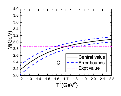
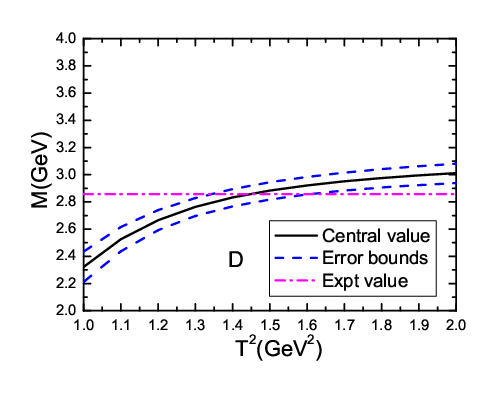
Figure 2: The masses of the charmed baryon states with variations of the Borel parameters T2T^{2}, where the AA, BB, CC and DD correspond to the charmed baryon states Ξc​(0,2,52)\Xi_{c}\left(0,2;\frac{5}{2}\right), Ξc​(0,2,32)\Xi_{c}\left(0,2;\frac{3}{2}\right), Λc​(0,2,52)\Lambda_{c}\left(0,2;\frac{5}{2}\right) and Λc​(0,2,32)\Lambda_{c}\left(0,2;\frac{3}{2}\right), respectively, the Expt value denotes the experimental values.
Refer to caption
Refer to caption
Refer to caption
Refer to caption
Figure 3: The masses of the charmed baryon states with variations of the Borel parameters T2T^{2}, where the AA, BB, CC and DD correspond to the charmed baryon states Ξc​(2,0,52)\Xi_{c}\left(2,0;\frac{5}{2}\right), Ξc​(2,0,32)\Xi_{c}\left(2,0;\frac{3}{2}\right), Λc​(2,0,52)\Lambda_{c}\left(2,0;\frac{5}{2}\right) and Λc​(2,0,32)\Lambda_{c}\left(2,0;\frac{3}{2}\right), respectively.
Refer to caption
Refer to caption
Refer to caption
Refer to caption
Figure 4: The masses of the charmed baryon states with variations of the Borel parameters T2T^{2}, where the AA, BB, CC and DD correspond to the charmed baryon states Ξc​(1,1,52)\Xi_{c}\left(1,1;\frac{5}{2}\right), Ξc​(1,1,32)\Xi_{c}\left(1,1;\frac{3}{2}\right), Λc​(1,1,52)\Lambda_{c}\left(1,1;\frac{5}{2}\right) and Λc​(1,1,32)\Lambda_{c}\left(1,1;\frac{3}{2}\right), respectively.
Refer to caption
Refer to caption
Refer to caption
Refer to caption
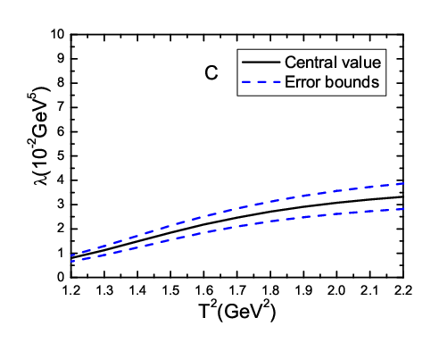
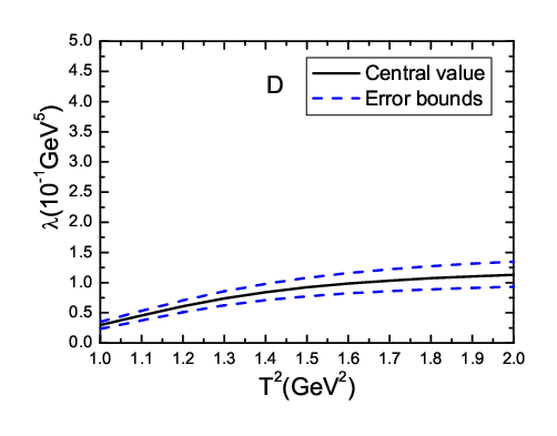
Figure 5: The pole residues of the charmed baryon states with variations of the Borel parameters T2T^{2}, where the AA, BB, CC and DD correspond to the charmed baryon states Ξc​(0,2,52)\Xi_{c}\left(0,2;\frac{5}{2}\right), Ξc​(0,2,32)\Xi_{c}\left(0,2;\frac{3}{2}\right), Λc​(0,2,52)\Lambda_{c}\left(0,2;\frac{5}{2}\right) and Λc​(0,2,32)\Lambda_{c}\left(0,2;\frac{3}{2}\right), respectively.
Refer to caption
Refer to caption
Refer to caption
Refer to caption
Figure 6: The pole residues of the charmed baryon states with variations of the Borel parameters T2T^{2}, where the AA, BB, CC and DD correspond to the charmed baryon states Ξc​(2,0,52)\Xi_{c}\left(2,0;\frac{5}{2}\right), Ξc​(2,0,32)\Xi_{c}\left(2,0;\frac{3}{2}\right), Λc​(2,0,52)\Lambda_{c}\left(2,0;\frac{5}{2}\right) and Λc​(2,0,32)\Lambda_{c}\left(2,0;\frac{3}{2}\right), respectively.
Refer to caption
Refer to caption
Refer to caption
Refer to caption
Figure 7: The pole residues of the charmed baryon states with variations of the Borel parameters T2T^{2}, where the AA, BB, CC and DD correspond to the charmed baryon states Ξc​(1,1,52)\Xi_{c}\left(1,1;\frac{5}{2}\right), Ξc​(1,1,32)\Xi_{c}\left(1,1;\frac{3}{2}\right), Λc​(1,1,52)\Lambda_{c}\left(1,1;\frac{5}{2}\right) and Λc​(1,1,32)\Lambda_{c}\left(1,1;\frac{3}{2}\right), respectively.

We take into account all uncertainties of the input parameters, and obtain the masses and pole residues of the D-wave charmed baryon states Λc\Lambda_{c} and Ξc\Xi_{c}, which are shown explicitly in Figs.2-7 and Table 2. In Figs.2-7, we plot the masses and pole residues with variations of the Borel parameters at much larger intervals than the Borel windows shown in Table 1. In the Borel windows, the uncertainties δ​M/M\delta M/M originate from the Borel parameters are very small, about (2−5)%(2-5)\%, the Borel platforms exist approximately. Furthermore, the energy scale formula μ=MB2−𝕄c2\mu=\sqrt{M_{B}^{2}-{\mathbb{M}}_{c}^{2}} is well satisfied. The criteria 𝟑\bf{3} and 𝟒\bf{4} are satisfied, now the four criteria are all satisfied.

In Fig.2 and Table 2, we also present the experimental values [1, 30] and predictions from the QCD sum rules combined with the heavy quark effective theory [8]. The present predictions are consistent with the experimental values [1, 30] and other QCD sum rules calculations [8], and support assigning the Λc​(2860)\Lambda_{c}(2860), Λc​(2880)\Lambda_{c}(2880), Ξc​(3055)\Xi_{c}(3055) and Ξc​(3080)\Xi_{c}(3080) to be the D-wave charmed baryon states with the quantum numbers (Lρ,Lλ)=(0,2)(L_{\rho},L_{\lambda})=(0,2) and JP=32+J^{P}={\frac{3}{2}}^{+}, 52+{\frac{5}{2}}^{+}, 32+{\frac{3}{2}}^{+} and 52+{\frac{5}{2}}^{+}, respectively. The predictions for the (Lρ,Lλ)=(2,0)(L_{\rho},L_{\lambda})=(2,0) and (Lρ,Lλ)=(1,1)(L_{\rho},L_{\lambda})=(1,1) D-wave Λc\Lambda_{c} and Ξc\Xi_{c} states can be confronted to the experimental data in the future.

4 Conclusion

In this article, we tentatively assign the Λc​(2860)\Lambda_{c}(2860), Λc​(2880)\Lambda_{c}(2880), Ξc​(3055)\Xi_{c}(3055) and Ξc​(3080)\Xi_{c}(3080) to be the D-wave charmed baryon states with JP=32+J^{P}={\frac{3}{2}}^{+}, 52+{\frac{5}{2}}^{+}, 32+{\frac{3}{2}}^{+} and 52+{\frac{5}{2}}^{+}, respectively, and study their masses and pole residues with the QCD sum rules in a systematic way by constructing three-types interpolating currents with the quantum numbers (Lρ,Lλ)=(0,2)(L_{\rho},L_{\lambda})=(0,2), (2,0)(2,0) and (1,1)(1,1), respectively. As the currents couple potentially to both the positive parity and negative parity baryon states, we separate the contributions of the 32±{\frac{3}{2}}^{\pm} and 52±{\frac{5}{2}}^{\pm} charmed baryon states unambiguously, and the QCD sum rules do not suffer from the contaminations of the charmed baryon states with negative parity. We carry out the operator product expansion up to the vacuum condensates of dimension 10 in a consistent way, and use the empirical energy scale formula to determine the optimal energy scales of the QCD spectral densities to extract the hadron masses. The present predictions support assigning the Λc​(2860)\Lambda_{c}(2860), Λc​(2880)\Lambda_{c}(2880), Ξc​(3055)\Xi_{c}(3055) and Ξc​(3080)\Xi_{c}(3080) to be the D-wave baryon states with the quantum numbers (Lρ,Lλ)=(0,2)(L_{\rho},L_{\lambda})=(0,2) and JP=32+J^{P}={\frac{3}{2}}^{+}, 52+{\frac{5}{2}}^{+}, 32+{\frac{3}{2}}^{+} and 52+{\frac{5}{2}}^{+}, respectively. The predictions for the masses of the (Lρ,Lλ)=(2,0)(L_{\rho},L_{\lambda})=(2,0) and (1,1)(1,1) D-wave Λc\Lambda_{c} and Ξc\Xi_{c} states can be confronted to the experimental data in the future.

Acknowledgements

This work is supported by National Natural Science Foundation, Grant Number 11375063.

Appendix

The explicit expressions of the QCD spectral densities ρj,Q​C​D0​(s)\rho^{0}_{j,QCD}(s) and ρj,Q​C​D1​(s)\rho^{1}_{j,QCD}(s),

ρj,Q​C​D0​(s)\displaystyle\rho^{0}_{j,QCD}(s) =\displaystyle= mc​ρj,Lρ,Lλ0;Ξc/Λc​(s),\displaystyle m_{c}\,\rho^{0;\Xi_{c}/\Lambda_{c}}_{j,L_{\rho},L_{\lambda}}(s)\,,
ρj,Q​C​D1​(s)\displaystyle\rho^{1}_{j,QCD}(s) =\displaystyle= ρj,Lρ,Lλ1;Ξc/Λc​(s),\displaystyle\rho^{1;\Xi_{c}/\Lambda_{c}}_{j,L_{\rho},L_{\lambda}}(s)\,, (36)
ρ52,2,00;Ξc​(s)\displaystyle\rho^{0;\Xi_{c}}_{{\frac{5}{2}},2,0}(s) =\displaystyle= 169120​π4​∫xi1d​x​(9​x2+34​x+132)​(1−x)4​(s−m~c2)4\displaystyle\frac{1}{69120\pi^{4}}\int_{x_{i}}^{1}dx\,(9x^{2}+34x+132)(1-x)^{4}(s-\widetilde{m}_{c}^{2})^{4} (37)
+5​ms​⟨s¯​s⟩−2​ms​⟨q¯​q⟩96​π2∫xi1dxx2(1−x)2(s−m~c2)2\displaystyle+\frac{5m_{s}\langle\bar{s}s\rangle-2m_{s}\langle\bar{q}q\rangle}{96\pi^{2}}\int_{x_{i}}^{1}dx\,x^{2}(1-x)^{2}(s-\widetilde{m}_{c}^{2})^{2}
+ms​⟨q¯​gs​σ​G​q⟩36​π2∫xi1dxx(3x−4)(1−x)(s−m~c2)\displaystyle+\frac{m_{s}\langle\bar{q}g_{s}\sigma Gq\rangle}{36\pi^{2}}\int_{x_{i}}^{1}dx\,x(3x-4)(1-x)(s-\widetilde{m}_{c}^{2})
+ms​⟨s¯​gs​σ​G​s⟩216​π2∫xi1dxx(31−27x)(1−x)(s−m~c2)\displaystyle+\frac{m_{s}\langle\bar{s}g_{s}\sigma Gs\rangle}{216\pi^{2}}\int_{x_{i}}^{1}dx\,x(31-27x)(1-x)(s-\widetilde{m}_{c}^{2})
−mc251840​π2⟨αs​G​Gπ⟩∫xi1dx(9​x2+34​x+132)​(1−x)4x3(s−m~c2)\displaystyle-\frac{m_{c}^{2}}{51840\pi^{2}}\langle\frac{\alpha_{s}GG}{\pi}\rangle\int_{x_{i}}^{1}dx\,\frac{(9x^{2}+34x+132)(1-x)^{4}}{x^{3}}(s-\widetilde{m}_{c}^{2})
+134560​π2⟨αs​G​Gπ⟩∫xi1dx(9​x2+34​x+132)​(1−x)4x2(s−m~c2)2\displaystyle+\frac{1}{34560\pi^{2}}\langle\frac{\alpha_{s}GG}{\pi}\rangle\int_{x_{i}}^{1}dx\,\frac{(9x^{2}+34x+132)(1-x)^{4}}{x^{2}}(s-\widetilde{m}_{c}^{2})^{2}
+16912​π2⟨αs​G​Gπ⟩∫xi1dx(9x2+20x+46)(1−x)2(s−m~c2)2\displaystyle+\frac{1}{6912\pi^{2}}\langle\frac{\alpha_{s}GG}{\pi}\rangle\int_{x_{i}}^{1}dx\,(9x^{2}+20x+46)(1-x)^{2}(s-\widetilde{m}_{c}^{2})^{2}
+⟨q¯​gs​σ​G​q⟩​⟨s¯​gs​σ​G​s⟩72​δ​(s−mc2),\displaystyle+\frac{\langle\bar{q}g_{s}\sigma Gq\rangle\langle\bar{s}g_{s}\sigma Gs\rangle}{72}\delta(s-m_{c}^{2})\,,
ρ52,2,01;Ξc​(s)\displaystyle\rho^{1;\Xi_{c}}_{{\frac{5}{2}},2,0}(s) =\displaystyle= 169120​π4​∫xi1d​x​x​(27​x2+55​x+128)​(1−x)4​(s−m~c2)4\displaystyle\frac{1}{69120\pi^{4}}\int_{x_{i}}^{1}dx\,x(27x^{2}+55x+128)(1-x)^{4}(s-\widetilde{m}_{c}^{2})^{4} (38)
+5​ms​⟨s¯​s⟩−2​ms​⟨q¯​q⟩288​π2∫xi1dxx2(9x−1)(1−x)2(s−m~c2)2\displaystyle+\frac{5m_{s}\langle\bar{s}s\rangle-2m_{s}\langle\bar{q}q\rangle}{288\pi^{2}}\int_{x_{i}}^{1}dx\,x^{2}(9x-1)(1-x)^{2}(s-\widetilde{m}_{c}^{2})^{2}
+ms​⟨q¯​gs​σ​G​q⟩72​π2∫xi1dxx(18x2−17x+1)(1−x)(s−m~c2)\displaystyle+\frac{m_{s}\langle\bar{q}g_{s}\sigma Gq\rangle}{72\pi^{2}}\int_{x_{i}}^{1}dx\,x(18x^{2}-17x+1)(1-x)(s-\widetilde{m}_{c}^{2})
+ms​⟨s¯​gs​σ​G​s⟩216​π2∫xi1dxx(−81x2+70x−4)(1−x)(s−m~c2)\displaystyle+\frac{m_{s}\langle\bar{s}g_{s}\sigma Gs\rangle}{216\pi^{2}}\int_{x_{i}}^{1}dx\,x(-81x^{2}+70x-4)(1-x)(s-\widetilde{m}_{c}^{2})
−mc251840​π2⟨αs​G​Gπ⟩∫xi1dx(27​x2+55​x+128)​(1−x)4x2(s−m~c2)\displaystyle-\frac{m_{c}^{2}}{51840\pi^{2}}\langle\frac{\alpha_{s}GG}{\pi}\rangle\int_{x_{i}}^{1}dx\,\frac{(27x^{2}+55x+128)(1-x)^{4}}{x^{2}}(s-\widetilde{m}_{c}^{2})
+16912​π2⟨αs​G​Gπ⟩∫xi1dxx(27x2+23x+40)(1−x)2(s−m~c2)2\displaystyle+\frac{1}{6912\pi^{2}}\langle\frac{\alpha_{s}GG}{\pi}\rangle\int_{x_{i}}^{1}dx\,x(27x^{2}+23x+40)(1-x)^{2}(s-\widetilde{m}_{c}^{2})^{2}
+5​⟨q¯​gs​σ​G​q⟩​⟨s¯​gs​σ​G​s⟩432​δ​(s−mc2),\displaystyle+\frac{5\langle\bar{q}g_{s}\sigma Gq\rangle\langle\bar{s}g_{s}\sigma Gs\rangle}{432}\delta(s-m_{c}^{2})\,,
ρ52,0,20;Ξc​(s)\displaystyle\rho^{0;\Xi_{c}}_{{\frac{5}{2}},0,2}(s) =\displaystyle= 14608​π4​∫xi1d​x​x​(3​x−2)​(1−x)4​(s−m~c2)4\displaystyle\frac{1}{4608\pi^{4}}\int_{x_{i}}^{1}dx\,x(3x-2)(1-x)^{4}(s-\widetilde{m}_{c}^{2})^{4} (39)
+ms​⟨s¯​s⟩−2​ms​⟨q¯​q⟩96​π2∫xi1dxx2(1−x)2(s−m~c2)2\displaystyle+\frac{m_{s}\langle\bar{s}s\rangle-2m_{s}\langle\bar{q}q\rangle}{96\pi^{2}}\int_{x_{i}}^{1}dx\,x^{2}(1-x)^{2}(s-\widetilde{m}_{c}^{2})^{2}
+mc23456​π2⟨αs​G​Gπ⟩∫xi1dx(2−3​x)​(1−x)4x2(s−m~c2)\displaystyle+\frac{m_{c}^{2}}{3456\pi^{2}}\langle\frac{\alpha_{s}GG}{\pi}\rangle\int_{x_{i}}^{1}dx\,\frac{(2-3x)(1-x)^{4}}{x^{2}}(s-\widetilde{m}_{c}^{2})
+12304​π2⟨αs​G​Gπ⟩∫xi1dx(3​x−2)​(1−x)4x(s−m~c2)2\displaystyle+\frac{1}{2304\pi^{2}}\langle\frac{\alpha_{s}GG}{\pi}\rangle\int_{x_{i}}^{1}dx\,\frac{(3x-2)(1-x)^{4}}{x}(s-\widetilde{m}_{c}^{2})^{2}
+1768​π2⟨αs​G​Gπ⟩∫xi1dxx2(1−x)2(s−m~c2)2\displaystyle+\frac{1}{768\pi^{2}}\langle\frac{\alpha_{s}GG}{\pi}\rangle\int_{x_{i}}^{1}dx\,x^{2}(1-x)^{2}(s-\widetilde{m}_{c}^{2})^{2}
+⟨q¯​gs​σ​G​q⟩​⟨s¯​gs​σ​G​s⟩72​δ​(s−mc2),\displaystyle+\frac{\langle\bar{q}g_{s}\sigma Gq\rangle\langle\bar{s}g_{s}\sigma Gs\rangle}{72}\delta(s-m_{c}^{2})\,,
ρ52,0,21;Ξc​(s)\displaystyle\rho^{1;\Xi_{c}}_{{\frac{5}{2}},0,2}(s) =\displaystyle= 14608​π4​∫xi1d​x​x2​(9​x+1)​(1−x)4​(s−m~c2)4\displaystyle\frac{1}{4608\pi^{4}}\int_{x_{i}}^{1}dx\,x^{2}(9x+1)(1-x)^{4}(s-\widetilde{m}_{c}^{2})^{4} (40)
+ms​⟨s¯​s⟩−2​ms​⟨q¯​q⟩288​π2∫xi1dxx2(9x−1)(1−x)2(s−m~c2)2\displaystyle+\frac{m_{s}\langle\bar{s}s\rangle-2m_{s}\langle\bar{q}q\rangle}{288\pi^{2}}\int_{x_{i}}^{1}dx\,x^{2}(9x-1)(1-x)^{2}(s-\widetilde{m}_{c}^{2})^{2}
−mc23456​π2⟨αs​G​Gπ⟩∫xi1dx(9​x+1)​(1−x)4x(s−m~c2)\displaystyle-\frac{m_{c}^{2}}{3456\pi^{2}}\langle\frac{\alpha_{s}GG}{\pi}\rangle\int_{x_{i}}^{1}dx\,\frac{(9x+1)(1-x)^{4}}{x}(s-\widetilde{m}_{c}^{2})
+12304​π2⟨αs​G​Gπ⟩∫xi1dxx2(9x−1)(1−x)2(s−m~c2)2\displaystyle+\frac{1}{2304\pi^{2}}\langle\frac{\alpha_{s}GG}{\pi}\rangle\int_{x_{i}}^{1}dx\,x^{2}(9x-1)(1-x)^{2}(s-\widetilde{m}_{c}^{2})^{2}
+5​⟨q¯​gs​σ​G​q⟩​⟨s¯​gs​σ​G​s⟩432​δ​(s−mc2),\displaystyle+\frac{5\langle\bar{q}g_{s}\sigma Gq\rangle\langle\bar{s}g_{s}\sigma Gs\rangle}{432}\delta(s-m_{c}^{2})\,,
ρ52,1,10;Ξc​(s)\displaystyle\rho^{0;\Xi_{c}}_{{\frac{5}{2}},1,1}(s) =\displaystyle= 113824​π4​∫xi1d​x​(3​x2+8​x−3)​(1−x)4​(s−m~c2)4\displaystyle\frac{1}{13824\pi^{4}}\int_{x_{i}}^{1}dx\,(3x^{2}+8x-3)(1-x)^{4}(s-\widetilde{m}_{c}^{2})^{4} (41)
+3​ms​⟨s¯​s⟩−2​ms​⟨q¯​q⟩96​π2∫xi1dxx2(1−x)2(s−m~c2)2\displaystyle+\frac{3m_{s}\langle\bar{s}s\rangle-2m_{s}\langle\bar{q}q\rangle}{96\pi^{2}}\int_{x_{i}}^{1}dx\,x^{2}(1-x)^{2}(s-\widetilde{m}_{c}^{2})^{2}
+ms​⟨q¯​gs​σ​G​q⟩48​π2∫xi1dxx(2x−1)(1−x)(s−m~c2)\displaystyle+\frac{m_{s}\langle\bar{q}g_{s}\sigma Gq\rangle}{48\pi^{2}}\int_{x_{i}}^{1}dx\,x(2x-1)(1-x)(s-\widetilde{m}_{c}^{2})
−5​ms​⟨s¯​gs​σ​G​s⟩432​π2∫xi1dxx(3x−1)(1−x)(s−m~c2)\displaystyle-\frac{5m_{s}\langle\bar{s}g_{s}\sigma Gs\rangle}{432\pi^{2}}\int_{x_{i}}^{1}dx\,x(3x-1)(1-x)(s-\widetilde{m}_{c}^{2})
−mc210368​π2⟨αs​G​Gπ⟩∫xi1dx(3​x2+8​x−3)​(1−x)4x3(s−m~c2)\displaystyle-\frac{m_{c}^{2}}{10368\pi^{2}}\langle\frac{\alpha_{s}GG}{\pi}\rangle\int_{x_{i}}^{1}dx\,\frac{(3x^{2}+8x-3)(1-x)^{4}}{x^{3}}(s-\widetilde{m}_{c}^{2})
+16912​π2⟨αs​G​Gπ⟩∫xi1dx(3​x2+8​x−3)​(1−x)4x2(s−m~c2)2\displaystyle+\frac{1}{6912\pi^{2}}\langle\frac{\alpha_{s}GG}{\pi}\rangle\int_{x_{i}}^{1}dx\,\frac{(3x^{2}+8x-3)(1-x)^{4}}{x^{2}}(s-\widetilde{m}_{c}^{2})^{2}
+14608​π2⟨αs​G​Gπ⟩∫xi1dx(6x2+10x−1)(1−x)2(s−m~c2)2,\displaystyle+\frac{1}{4608\pi^{2}}\langle\frac{\alpha_{s}GG}{\pi}\rangle\int_{x_{i}}^{1}dx\,(6x^{2}+10x-1)(1-x)^{2}(s-\widetilde{m}_{c}^{2})^{2}\,,
ρ52,1,11;Ξc​(s)\displaystyle\rho^{1;\Xi_{c}}_{{\frac{5}{2}},1,1}(s) =\displaystyle= 113824​π4​∫xi1d​x​x​(9​x2+14​x+2)​(1−x)4​(s−m~c2)4\displaystyle\frac{1}{13824\pi^{4}}\int_{x_{i}}^{1}dx\,x(9x^{2}+14x+2)(1-x)^{4}(s-\widetilde{m}_{c}^{2})^{4} (42)
+3​ms​⟨s¯​s⟩−2​ms​⟨q¯​q⟩288​π2∫xi1dxx2(9x−1)(1−x)2(s−m~c2)2\displaystyle+\frac{3m_{s}\langle\bar{s}s\rangle-2m_{s}\langle\bar{q}q\rangle}{288\pi^{2}}\int_{x_{i}}^{1}dx\,x^{2}(9x-1)(1-x)^{2}(s-\widetilde{m}_{c}^{2})^{2}
+ms​⟨q¯​gs​σ​G​q⟩288​π2∫xi1dxx(36x2−21x+1)(1−x)(s−m~c2)\displaystyle+\frac{m_{s}\langle\bar{q}g_{s}\sigma Gq\rangle}{288\pi^{2}}\int_{x_{i}}^{1}dx\,x(36x^{2}-21x+1)(1-x)(s-\widetilde{m}_{c}^{2})
+ms​⟨s¯​gs​σ​G​s⟩432​π2∫xi1dxx(−45x2+23x−1)(1−x)(s−m~c2)\displaystyle+\frac{m_{s}\langle\bar{s}g_{s}\sigma Gs\rangle}{432\pi^{2}}\int_{x_{i}}^{1}dx\,x(-45x^{2}+23x-1)(1-x)(s-\widetilde{m}_{c}^{2})
−mc210368​π2⟨αs​G​Gπ⟩∫xi1dx(9​x2+14​x+2)​(1−x)4x2(s−m~c2)\displaystyle-\frac{m_{c}^{2}}{10368\pi^{2}}\langle\frac{\alpha_{s}GG}{\pi}\rangle\int_{x_{i}}^{1}dx\,\frac{(9x^{2}+14x+2)(1-x)^{4}}{x^{2}}(s-\widetilde{m}_{c}^{2})
+14608​π2⟨αs​G​Gπ⟩∫xi1dxx2(18x+11)(1−x)2(s−m~c2)2,\displaystyle+\frac{1}{4608\pi^{2}}\langle\frac{\alpha_{s}GG}{\pi}\rangle\int_{x_{i}}^{1}dx\,x^{2}(18x+11)(1-x)^{2}(s-\widetilde{m}_{c}^{2})^{2}\,,
ρ32,2,00;Ξc​(s)\displaystyle\rho^{0;\Xi_{c}}_{{\frac{3}{2}},2,0}(s) =\displaystyle= 13072​π4​∫xi1d​x​(4​x+33)​(1−x)4​(s−m~c2)4\displaystyle\frac{1}{3072\pi^{4}}\int_{x_{i}}^{1}dx\,(4x+33)(1-x)^{4}(s-\widetilde{m}_{c}^{2})^{4} (43)
+7​ms​⟨s¯​gs​σ​G​s⟩−6​ms​⟨q¯​gs​σ​G​q⟩24​π2∫xi1dxx(1−x)(s−m~c2)\displaystyle+\frac{7m_{s}\langle\bar{s}g_{s}\sigma Gs\rangle-6m_{s}\langle\bar{q}g_{s}\sigma Gq\rangle}{24\pi^{2}}\int_{x_{i}}^{1}dx\,x(1-x)(s-\widetilde{m}_{c}^{2})
−mc22304​π2⟨αs​G​Gπ⟩∫xi1dx(4​x+33)​(1−x)4x3(s−m~c2)\displaystyle-\frac{m_{c}^{2}}{2304\pi^{2}}\langle\frac{\alpha_{s}GG}{\pi}\rangle\int_{x_{i}}^{1}dx\,\frac{(4x+33)(1-x)^{4}}{x^{3}}(s-\widetilde{m}_{c}^{2})
+11536​π2⟨αs​G​Gπ⟩∫xi1dx(4​x+33)​(1−x)4x2(s−m~c2)2\displaystyle+\frac{1}{1536\pi^{2}}\langle\frac{\alpha_{s}GG}{\pi}\rangle\int_{x_{i}}^{1}dx\,\frac{(4x+33)(1-x)^{4}}{x^{2}}(s-\widetilde{m}_{c}^{2})^{2}
+1768​π2⟨αs​G​Gπ⟩∫xi1dx(8x+31)(1−x)2(s−m~c2)2\displaystyle+\frac{1}{768\pi^{2}}\langle\frac{\alpha_{s}GG}{\pi}\rangle\int_{x_{i}}^{1}dx\,(8x+31)(1-x)^{2}(s-\widetilde{m}_{c}^{2})^{2}
+3​⟨q¯​gs​σ​G​q⟩​⟨s¯​gs​σ​G​s⟩32​δ​(s−mc2),\displaystyle+\frac{3\langle\bar{q}g_{s}\sigma Gq\rangle\langle\bar{s}g_{s}\sigma Gs\rangle}{32}\delta(s-m_{c}^{2})\,,
ρ32,2,01;Ξc​(s)\displaystyle\rho^{1;\Xi_{c}}_{{\frac{3}{2}},2,0}(s) =\displaystyle= 53072​π4​∫xi1d​x​x​(4​x+9)​(1−x)4​(s−m~c2)4\displaystyle\frac{5}{3072\pi^{4}}\int_{x_{i}}^{1}dx\,x(4x+9)(1-x)^{4}(s-\widetilde{m}_{c}^{2})^{4} (44)
+25​ms​⟨s¯​s⟩−10​ms​⟨q¯​q⟩16​π2∫xi1dxx2(1−x)2(s−m~c2)2\displaystyle+\frac{25m_{s}\langle\bar{s}s\rangle-10m_{s}\langle\bar{q}q\rangle}{16\pi^{2}}\int_{x_{i}}^{1}dx\,x^{2}(1-x)^{2}(s-\widetilde{m}_{c}^{2})^{2}
+ms​⟨q¯​gs​σ​G​q⟩4​π2∫xi1dxx(7x−4)(1−x)(s−m~c2)\displaystyle+\frac{m_{s}\langle\bar{q}g_{s}\sigma Gq\rangle}{4\pi^{2}}\int_{x_{i}}^{1}dx\,x(7x-4)(1-x)(s-\widetilde{m}_{c}^{2})
+ms​⟨s¯​gs​σ​G​s⟩24​π2∫xi1dxx(33−64x)(1−x)(s−m~c2)\displaystyle+\frac{m_{s}\langle\bar{s}g_{s}\sigma Gs\rangle}{24\pi^{2}}\int_{x_{i}}^{1}dx\,x(33-64x)(1-x)(s-\widetilde{m}_{c}^{2})
−5​mc22304​π2⟨αs​G​Gπ⟩∫xi1dx(4​x+9)​(1−x)4x2(s−m~c2)\displaystyle-\frac{5m_{c}^{2}}{2304\pi^{2}}\langle\frac{\alpha_{s}GG}{\pi}\rangle\int_{x_{i}}^{1}dx\,\frac{(4x+9)(1-x)^{4}}{x^{2}}(s-\widetilde{m}_{c}^{2})
+1768​π2⟨αs​G​Gπ⟩∫xi1dxx(34x+35)(1−x)2(s−m~c2)2\displaystyle+\frac{1}{768\pi^{2}}\langle\frac{\alpha_{s}GG}{\pi}\rangle\int_{x_{i}}^{1}dx\,x(34x+35)(1-x)^{2}(s-\widetilde{m}_{c}^{2})^{2}
+5​⟨q¯​gs​σ​G​q⟩​⟨s¯​gs​σ​G​s⟩96​δ​(s−mc2),\displaystyle+\frac{5\langle\bar{q}g_{s}\sigma Gq\rangle\langle\bar{s}g_{s}\sigma Gs\rangle}{96}\delta(s-m_{c}^{2})\,,
ρ32,0,20;Ξc​(s)\displaystyle\rho^{0;\Xi_{c}}_{{\frac{3}{2}},0,2}(s) =\displaystyle= 11024​π4​∫xi1d​x​(3−4​x)​(1−x)4​(s−m~c2)4\displaystyle\frac{1}{1024\pi^{4}}\int_{x_{i}}^{1}dx\,(3-4x)(1-x)^{4}(s-\widetilde{m}_{c}^{2})^{4} (45)
−mc2768​π2⟨αs​G​Gπ⟩∫xi1dx(3−4​x)​(1−x)4x3(s−m~c2)\displaystyle-\frac{m_{c}^{2}}{768\pi^{2}}\langle\frac{\alpha_{s}GG}{\pi}\rangle\int_{x_{i}}^{1}dx\,\frac{(3-4x)(1-x)^{4}}{x^{3}}(s-\widetilde{m}_{c}^{2})
+1512​π2⟨αs​G​Gπ⟩∫xi1dx(3−4​x)​(1−x)4x2(s−m~c2)2\displaystyle+\frac{1}{512\pi^{2}}\langle\frac{\alpha_{s}GG}{\pi}\rangle\int_{x_{i}}^{1}dx\,\frac{(3-4x)(1-x)^{4}}{x^{2}}(s-\widetilde{m}_{c}^{2})^{2}
+3​⟨q¯​gs​σ​G​q⟩​⟨s¯​gs​σ​G​s⟩32​δ​(s−mc2),\displaystyle+\frac{3\langle\bar{q}g_{s}\sigma Gq\rangle\langle\bar{s}g_{s}\sigma Gs\rangle}{32}\delta(s-m_{c}^{2})\,,
ρ32,0,21;Ξc​(s)\displaystyle\rho^{1;\Xi_{c}}_{{\frac{3}{2}},0,2}(s) =\displaystyle= 71024​π4​∫xi1d​x​x​(4​x+1)​(1−x)4​(s−m~c2)4\displaystyle\frac{7}{1024\pi^{4}}\int_{x_{i}}^{1}dx\,x(4x+1)(1-x)^{4}(s-\widetilde{m}_{c}^{2})^{4} (46)
+5​ms​⟨s¯​s⟩−10​ms​⟨q¯​q⟩16​π2∫xi1dxx2(1−x)2(s−m~c2)2\displaystyle+\frac{5m_{s}\langle\bar{s}s\rangle-10m_{s}\langle\bar{q}q\rangle}{16\pi^{2}}\int_{x_{i}}^{1}dx\,x^{2}(1-x)^{2}(s-\widetilde{m}_{c}^{2})^{2}
−7​mc2768​π2⟨αs​G​Gπ⟩∫xi1dx(4​x+1)​(1−x)4x2(s−m~c2)\displaystyle-\frac{7m_{c}^{2}}{768\pi^{2}}\langle\frac{\alpha_{s}GG}{\pi}\rangle\int_{x_{i}}^{1}dx\,\frac{(4x+1)(1-x)^{4}}{x^{2}}(s-\widetilde{m}_{c}^{2})
+5128​π2⟨αs​G​Gπ⟩∫xi1dxx2(1−x)2(s−m~c2)2\displaystyle+\frac{5}{128\pi^{2}}\langle\frac{\alpha_{s}GG}{\pi}\rangle\int_{x_{i}}^{1}dx\,x^{2}(1-x)^{2}(s-\widetilde{m}_{c}^{2})^{2}
+5​⟨q¯​gs​σ​G​q⟩​⟨s¯​gs​σ​G​s⟩96​δ​(s−mc2),\displaystyle+\frac{5\langle\bar{q}g_{s}\sigma Gq\rangle\langle\bar{s}g_{s}\sigma Gs\rangle}{96}\delta(s-m_{c}^{2})\,,
ρ32,1,10;Ξc​(s)\displaystyle\rho^{0;\Xi_{c}}_{{\frac{3}{2}},1,1}(s) =\displaystyle= 1768​π4​∫xi1d​x​(x−3)​(1−x)4​(s−m~c2)4\displaystyle\frac{1}{768\pi^{4}}\int_{x_{i}}^{1}dx\,(x-3)(1-x)^{4}(s-\widetilde{m}_{c}^{2})^{4} (47)
−ms​⟨s¯​gs​σ​G​s⟩48​π2∫xi1dxx(1−x)(s−m~c2)\displaystyle-\frac{m_{s}\langle\bar{s}g_{s}\sigma Gs\rangle}{48\pi^{2}}\int_{x_{i}}^{1}dx\,x(1-x)(s-\widetilde{m}_{c}^{2})
−mc2576​π2⟨αs​G​Gπ⟩∫xi1dx(x−3)​(1−x)4x3(s−m~c2)\displaystyle-\frac{m_{c}^{2}}{576\pi^{2}}\langle\frac{\alpha_{s}GG}{\pi}\rangle\int_{x_{i}}^{1}dx\,\frac{(x-3)(1-x)^{4}}{x^{3}}(s-\widetilde{m}_{c}^{2})
+1384​π2⟨αs​G​Gπ⟩∫xi1dx(x−3)​(1−x)4x2(s−m~c2)2\displaystyle+\frac{1}{384\pi^{2}}\langle\frac{\alpha_{s}GG}{\pi}\rangle\int_{x_{i}}^{1}dx\,\frac{(x-3)(1-x)^{4}}{x^{2}}(s-\widetilde{m}_{c}^{2})^{2}
+11024​π2⟨αs​G​Gπ⟩∫xi1dx(8x−5)(1−x)2(s−m~c2)2,\displaystyle+\frac{1}{1024\pi^{2}}\langle\frac{\alpha_{s}GG}{\pi}\rangle\int_{x_{i}}^{1}dx\,(8x-5)(1-x)^{2}(s-\widetilde{m}_{c}^{2})^{2}\,,
ρ32,1,11;Ξc​(s)\displaystyle\rho^{1;\Xi_{c}}_{{\frac{3}{2}},1,1}(s) =\displaystyle= 1768​π4​∫xi1d​x​x​(8​x+7)​(1−x)4​(s−m~c2)4\displaystyle\frac{1}{768\pi^{4}}\int_{x_{i}}^{1}dx\,x(8x+7)(1-x)^{4}(s-\widetilde{m}_{c}^{2})^{4} (48)
+15​ms​⟨s¯​s⟩−10​ms​⟨q¯​q⟩16​π2∫xi1dxx2(1−x)2(s−m~c2)2\displaystyle+\frac{15m_{s}\langle\bar{s}s\rangle-10m_{s}\langle\bar{q}q\rangle}{16\pi^{2}}\int_{x_{i}}^{1}dx\,x^{2}(1-x)^{2}(s-\widetilde{m}_{c}^{2})^{2}
+5​ms​⟨q¯​gs​σ​G​q⟩16​π2∫xi1dxx(3x−1)(1−x)(s−m~c2)\displaystyle+\frac{5m_{s}\langle\bar{q}g_{s}\sigma Gq\rangle}{16\pi^{2}}\int_{x_{i}}^{1}dx\,x(3x-1)(1-x)(s-\widetilde{m}_{c}^{2})
+ms​⟨s¯​gs​σ​G​s⟩48​π2∫xi1dxx(11−38x)(1−x)(s−m~c2)\displaystyle+\frac{m_{s}\langle\bar{s}g_{s}\sigma Gs\rangle}{48\pi^{2}}\int_{x_{i}}^{1}dx\,x(11-38x)(1-x)(s-\widetilde{m}_{c}^{2})
−mc2576​π2⟨αs​G​Gπ⟩∫xi1dx(8​x+7)​(1−x)4x2(s−m~c2)\displaystyle-\frac{m_{c}^{2}}{576\pi^{2}}\langle\frac{\alpha_{s}GG}{\pi}\rangle\int_{x_{i}}^{1}dx\,\frac{(8x+7)(1-x)^{4}}{x^{2}}(s-\widetilde{m}_{c}^{2})
+11024​π2⟨αs​G​Gπ⟩∫xi1dxx(44x+15)(1−x)2(s−m~c2)2,\displaystyle+\frac{1}{1024\pi^{2}}\langle\frac{\alpha_{s}GG}{\pi}\rangle\int_{x_{i}}^{1}dx\,x(44x+15)(1-x)^{2}(s-\widetilde{m}_{c}^{2})^{2}\,,
ρ52,2,00;Λc​(s)\displaystyle\rho^{0;\Lambda_{c}}_{{\frac{5}{2}},2,0}(s) =\displaystyle= ρ52,2,00;Ξc​(s)∣ms→0,⟨s¯​s⟩→⟨q¯​q⟩,⟨s¯​gs​σ​G​s⟩→⟨q¯​gs​σ​G​q⟩,\displaystyle\rho^{0;\Xi_{c}}_{{\frac{5}{2}},2,0}(s)\mid_{m_{s}\to 0,\,\,\langle\bar{s}s\rangle\to\langle\bar{q}q\rangle,\,\,\langle\bar{s}g_{s}\sigma Gs\rangle\to\langle\bar{q}g_{s}\sigma Gq\rangle}\,,
ρ52,0,20;Λc​(s)\displaystyle\rho^{0;\Lambda_{c}}_{{\frac{5}{2}},0,2}(s) =\displaystyle= ρ52,0,20;Ξc​(s)∣ms→0,⟨s¯​s⟩→⟨q¯​q⟩,⟨s¯​gs​σ​G​s⟩→⟨q¯​gs​σ​G​q⟩,\displaystyle\rho^{0;\Xi_{c}}_{{\frac{5}{2}},0,2}(s)\mid_{m_{s}\to 0,\,\,\langle\bar{s}s\rangle\to\langle\bar{q}q\rangle,\,\,\langle\bar{s}g_{s}\sigma Gs\rangle\to\langle\bar{q}g_{s}\sigma Gq\rangle}\,,
ρ52,1,10;Λc​(s)\displaystyle\rho^{0;\Lambda_{c}}_{{\frac{5}{2}},1,1}(s) =\displaystyle= ρ52,1,10;Ξc​(s)∣ms→0,⟨s¯​s⟩→⟨q¯​q⟩,⟨s¯​gs​σ​G​s⟩→⟨q¯​gs​σ​G​q⟩,\displaystyle\rho^{0;\Xi_{c}}_{{\frac{5}{2}},1,1}(s)\mid_{m_{s}\to 0,\,\,\langle\bar{s}s\rangle\to\langle\bar{q}q\rangle,\,\,\langle\bar{s}g_{s}\sigma Gs\rangle\to\langle\bar{q}g_{s}\sigma Gq\rangle}\,,
ρ52,2,01;Λc​(s)\displaystyle\rho^{1;\Lambda_{c}}_{{\frac{5}{2}},2,0}(s) =\displaystyle= ρ52,2,01;Ξc​(s)∣ms→0,⟨s¯​s⟩→⟨q¯​q⟩,⟨s¯​gs​σ​G​s⟩→⟨q¯​gs​σ​G​q⟩,\displaystyle\rho^{1;\Xi_{c}}_{{\frac{5}{2}},2,0}(s)\mid_{m_{s}\to 0,\,\,\langle\bar{s}s\rangle\to\langle\bar{q}q\rangle,\,\,\langle\bar{s}g_{s}\sigma Gs\rangle\to\langle\bar{q}g_{s}\sigma Gq\rangle}\,,
ρ52,0,21;Λc​(s)\displaystyle\rho^{1;\Lambda_{c}}_{{\frac{5}{2}},0,2}(s) =\displaystyle= ρ52,0,21;Ξc​(s)∣ms→0,⟨s¯​s⟩→⟨q¯​q⟩,⟨s¯​gs​σ​G​s⟩→⟨q¯​gs​σ​G​q⟩,\displaystyle\rho^{1;\Xi_{c}}_{{\frac{5}{2}},0,2}(s)\mid_{m_{s}\to 0,\,\,\langle\bar{s}s\rangle\to\langle\bar{q}q\rangle,\,\,\langle\bar{s}g_{s}\sigma Gs\rangle\to\langle\bar{q}g_{s}\sigma Gq\rangle}\,,
ρ52,1,11;Λc​(s)\displaystyle\rho^{1;\Lambda_{c}}_{{\frac{5}{2}},1,1}(s) =\displaystyle= ρ52,1,11;Ξc​(s)∣ms→0,⟨s¯​s⟩→⟨q¯​q⟩,⟨s¯​gs​σ​G​s⟩→⟨q¯​gs​σ​G​q⟩,\displaystyle\rho^{1;\Xi_{c}}_{{\frac{5}{2}},1,1}(s)\mid_{m_{s}\to 0,\,\,\langle\bar{s}s\rangle\to\langle\bar{q}q\rangle,\,\,\langle\bar{s}g_{s}\sigma Gs\rangle\to\langle\bar{q}g_{s}\sigma Gq\rangle}\,, (49)
ρ32,2,00;Λc​(s)\displaystyle\rho^{0;\Lambda_{c}}_{{\frac{3}{2}},2,0}(s) =\displaystyle= ρ32,2,00;Ξc​(s)∣ms→0,⟨s¯​s⟩→⟨q¯​q⟩,⟨s¯​gs​σ​G​s⟩→⟨q¯​gs​σ​G​q⟩,\displaystyle\rho^{0;\Xi_{c}}_{{\frac{3}{2}},2,0}(s)\mid_{m_{s}\to 0,\,\,\langle\bar{s}s\rangle\to\langle\bar{q}q\rangle,\,\,\langle\bar{s}g_{s}\sigma Gs\rangle\to\langle\bar{q}g_{s}\sigma Gq\rangle}\,,
ρ32,0,20;Λc​(s)\displaystyle\rho^{0;\Lambda_{c}}_{{\frac{3}{2}},0,2}(s) =\displaystyle= ρ32,0,20;Ξc​(s)∣ms→0,⟨s¯​s⟩→⟨q¯​q⟩,⟨s¯​gs​σ​G​s⟩→⟨q¯​gs​σ​G​q⟩,\displaystyle\rho^{0;\Xi_{c}}_{{\frac{3}{2}},0,2}(s)\mid_{m_{s}\to 0,\,\,\langle\bar{s}s\rangle\to\langle\bar{q}q\rangle,\,\,\langle\bar{s}g_{s}\sigma Gs\rangle\to\langle\bar{q}g_{s}\sigma Gq\rangle}\,,
ρ32,1,10;Λc​(s)\displaystyle\rho^{0;\Lambda_{c}}_{{\frac{3}{2}},1,1}(s) =\displaystyle= ρ32,1,10;Ξc​(s)∣ms→0,⟨s¯​s⟩→⟨q¯​q⟩,⟨s¯​gs​σ​G​s⟩→⟨q¯​gs​σ​G​q⟩,\displaystyle\rho^{0;\Xi_{c}}_{{\frac{3}{2}},1,1}(s)\mid_{m_{s}\to 0,\,\,\langle\bar{s}s\rangle\to\langle\bar{q}q\rangle,\,\,\langle\bar{s}g_{s}\sigma Gs\rangle\to\langle\bar{q}g_{s}\sigma Gq\rangle}\,,
ρ32,2,01;Λc​(s)\displaystyle\rho^{1;\Lambda_{c}}_{{\frac{3}{2}},2,0}(s) =\displaystyle= ρ32,2,01;Ξc​(s)∣ms→0,⟨s¯​s⟩→⟨q¯​q⟩,⟨s¯​gs​σ​G​s⟩→⟨q¯​gs​σ​G​q⟩,\displaystyle\rho^{1;\Xi_{c}}_{{\frac{3}{2}},2,0}(s)\mid_{m_{s}\to 0,\,\,\langle\bar{s}s\rangle\to\langle\bar{q}q\rangle,\,\,\langle\bar{s}g_{s}\sigma Gs\rangle\to\langle\bar{q}g_{s}\sigma Gq\rangle}\,,
ρ32,0,21;Λc​(s)\displaystyle\rho^{1;\Lambda_{c}}_{{\frac{3}{2}},0,2}(s) =\displaystyle= ρ32,0,21;Ξc​(s)∣ms→0,⟨s¯​s⟩→⟨q¯​q⟩,⟨s¯​gs​σ​G​s⟩→⟨q¯​gs​σ​G​q⟩,\displaystyle\rho^{1;\Xi_{c}}_{{\frac{3}{2}},0,2}(s)\mid_{m_{s}\to 0,\,\,\langle\bar{s}s\rangle\to\langle\bar{q}q\rangle,\,\,\langle\bar{s}g_{s}\sigma Gs\rangle\to\langle\bar{q}g_{s}\sigma Gq\rangle}\,,
ρ32,1,11;Λc​(s)\displaystyle\rho^{1;\Lambda_{c}}_{{\frac{3}{2}},1,1}(s) =\displaystyle= ρ32,1,11;Ξc​(s)∣ms→0,⟨s¯​s⟩→⟨q¯​q⟩,⟨s¯​gs​σ​G​s⟩→⟨q¯​gs​σ​G​q⟩,\displaystyle\rho^{1;\Xi_{c}}_{{\frac{3}{2}},1,1}(s)\mid_{m_{s}\to 0,\,\,\langle\bar{s}s\rangle\to\langle\bar{q}q\rangle,\,\,\langle\bar{s}g_{s}\sigma Gs\rangle\to\langle\bar{q}g_{s}\sigma Gq\rangle}\,, (50)

m~c2=mc2x\widetilde{m}_{c}^{2}=\frac{m_{c}^{2}}{x}, xi=mc2sx_{i}=\frac{m_{c}^{2}}{s}.

References

  • [1] R. Aaij et al, JHEP 1705 (2017) 030.
  • [2] M. Artuso et al, Phys. Rev. Lett. 86 (2001) 4479.
  • [3] B. Aubert et al, Phys. Rev. Lett. 98 (2007) 012001.
  • [4] R. Mizuk et al, Phys. Rev. Lett. 98 (2007) 262001.
  • [5] W. Roberts and M. Pervin, Int. J. Mod. Phys. A23 (2008) 2817.
  • [6] D. Ebert, R. N. Faustov and V. O. Galkin, Phys. Rev. D84 (2011) 014025.
  • [7] Z. Shah, K. Thakkar, A. K. Rai and P. C. Vinodkumar, Eur. Phys. J. A52 (2016) 313.
  • [8] H. X. Chen, Q. Mao, A. Hosaka, X. Liu and S. L. Zhu, Phys. Rev. D94 (2016) 114016.
  • [9] B. Chen, K. W. Wei, X. Liu and T. Matsuki, Eur. Phys. J. C77 (2017) 154.
  • [10] B. Chen, X. Liu and A. Zhang, Phys. Rev. D95 (2017) 074022.
  • [11] R. Chistov et al, Phys. Rev. Lett. 97 (2006) 162001.
  • [12] B. Aubert et al, Phys. Rev. D77 (2008) 012002.
  • [13] Y. Kato et al, Phys. Rev. D94 (2016) 032002.
  • [14] Z. G. Wang, Eur. Phys. J. A47 (2011) 81.
  • [15] Z. G. Wang, Commun. Theor. Phys. 58 (2012) 723.
  • [16] T. M. Aliev, K. Azizi and M. Savci, J. Phys. G40 (2013) 065003; K. Azizi and H. Sundu, Eur. Phys. J. Plus 132 (2017) 22.
  • [17] Z. G. Wang, Phys. Lett. B685 (2010) 59; Z. G. Wang, Eur. Phys. J. C68 (2010) 459; Z. G. Wang, Eur. Phys. J. A45 (2010) 267.
  • [18] H. X. Chen, W. Chen, Q. Mao, A. Hosaka, X. Liu and S. L. Zhu, Phys. Rev. D91 (2015) 054034; Q. Mao, H. X. Chen, W. Chen, A. Hosaka, X. Liu and S. L. Zhu, Phys. Rev. D92 (2015) 114007.
  • [19] Z. G. Wang, Eur. Phys. J. C75 (2015) 359.
  • [20] A. De Rujula, H. Georgi and S. L. Glashow, Phys. Rev. D12 (1975) 147; T. DeGrand, R. L. Jaffe, K. Johnson and J. E. Kiskis, Phys. Rev. D12 (1975) 2060.
  • [21] Z. G. Wang, Commun. Theor. Phys. 59 (2013) 451.
  • [22] J. G. Korner, M. Kramer and D. Pirjol, Prog. Part. Nucl. Phys. 33 (1994) 787.
  • [23] Z. G. Wang and Z. Y. Di, Eur. Phys. J. A50 (2014) 143.
  • [24] Y. Chung, H. G. Dosch, M. Kremer and D. Schall, Nucl. Phys. B197 (1982) 55; D. Jido, N. Kodama and M. Oka, Phys. Rev. D54 (1996) 4532.
  • [25] Z. G. Wang, Eur. Phys. J. C76 (2016) 70.
  • [26] M. A. Shifman, A. I. Vainshtein and V. I. Zakharov, Nucl. Phys. B147 (1979) 385, 448.
  • [27] L. J. Reinders, H. Rubinstein and S. Yazaki, Phys. Rept. 127 (1985) 1.
  • [28] Shi-Zhong Huang, ”Free particles and fields of high spins” (in chinese), Anhui peoples Publishing House, 2006.
  • [29] P. Colangelo and A. Khodjamirian, hep-ph/0010175.
  • [30] C. Patrignani et al, Chin. Phys. C40 (2016) 100001.
  • [31] Z. G. Wang and T. Huang, Phys. Rev. D89 (2014) 054019; Z. G. Wang, Eur. Phys. J. C74 (2014) 2874; Z. G. Wang and T. Huang, Nucl. Phys. A930 (2014)63.
  • [32] Z. G. Wang and T. Huang, Eur. Phys. J. C74 (2014) 2891; Z. G. Wang, Eur. Phys. J. C74 (2014) 2963.
  • [33] Z. G. Wang, Int. J. Mod. Phys. A30 (2015) 1550168.
  • [34] Z. G. Wang, Eur. Phys. J. C77 (2017) 325.
  • [35] Z. G. Wang, Eur. Phys. J. C77 (2017) 174; Z. G. Wang, Eur. Phys. J. A53 (2017) 192.
  • [36] Z. G. Wang, Eur. Phys. J. C76 (2016) 387.
  • [37] Y. J. Xu, Y. L. Liu and M. Q. Huang, Commun. Theor. Phys. 63 (2015) 209.