跳到论文正文
W Papers独立论文阅读器 arXiv:1705.07566 论文正文 计算阅读时间 · 0%
引用这篇论文根据当前论文元数据生成,正式投稿前建议核对。


License: arXiv.org perpetual non-exclusive license
arXiv:1705.07566v3 [math.PR] 31 May 2017

Hypergroups derived from random walks on some infinite graphs

Tomohiro IKKAI Note: e-mail: m13006z@math.nagoya-u.ac.jp    Yusuke SAWADA Note: e-mail: m14017c@math.nagoya-u.ac.jp
Abstract

Wildberger gave a method to construct a finite hermitian discrete hypergroup from a random walk on a certain kind of finite graphs. In this article, we reveal that his method is applicable to a random walk on a certain kind of infinite graphs. Moreover, we make some observations of finite or infinite graphs on which a random walk produces a hermitian discrete hypergroup.

Graduate School of Mathematics,

Nagoya University,

Nagoya, 464-8602, JAPAN

†† 2010 Mathematics Subject Classification: Primary 43A62; Secondary 05C81.†† Key words and phrases: Hermitian discrete hypergroups, distance-regular graphs, association schemes, Cayley graphs, infinite graphs.

1 Introduction

Let ℕ\mathbb{N} be the set of positive integers, ℕ0=ℕ∪{0}\mathbb{N}_{0}=\mathbb{N}\cup\{0\}, ℤ\mathbb{Z} be the ring of rational integers, ℝ\mathbb{R} be the field of real numbers, ℝ+\mathbb{R}_{+} be the set of non-negative real numbers and ℂ\mathbb{C} be the field of complex numbers, respectively.

The concept of hypergroups is a probability theoretic extension of the concept of locally compact groups. It was introduced by Dunkl [5], Jewett [6] and Spector [11], and many authors developed harmonic analysis and representation theory on hypergroups as well as those on locally compact groups.

Discrete hypergroups, including finite hypergroups, are the main objects in this article. We state the definition of discrete hypergroups in Section 2.1, but omit the general definition of the non-discrete cases in this article. For the general definition of hypergroups and a fundamental theory of hypergroups, see [3] for example. Actually, the concept of (finite) discrete hypergroups was implicitly utilized by Frobenius around 1900, before Dunkl, Jewett and Spector. Recently, it was shown by Wildberger [14] that finite commutative hypergroups have some connections with number theory, conformal field theory, subfactor theory and other fields.

Structures of finite hypergroups of order two and three are completely determined. Indeed, those of order two are classically known, and those of order three were investigated by Wildberger [15]. However, few examples of finite hypergroups of order four or greater were known; A recent result by Matsuzawa, Ohno, Suzuki, Tsurii and Yamanaka [9] gives some examples of non-commutative hypergroups of order five. Wildberger [13], [14] gave a way to construct a finite commutative hypergroup from a random walk on a certain kind of finite graphs. By his method, we have some examples of hypergroups of large order. In particular, the authors disclose that random walks on prism graphs produce finite commutative hypergroups of arbitrarily large order. After recalling Wildberger’s method in Section 3, we will give the structures of those hypergroups derived from prism graphs in Section 4.2.

It is known that not all finite graphs produce hypergroups. Wildberger mentioned that a random walk on any strong regular graph and on any distance transitive graph produces a hypergroup of order three and suggested that a random walk on any distance-regular graphs produces a finite hypergroup. (We do not discuss on distance transitive graphs in this article, but it is known that distance transitive graphs are always distance-regular.) The authors verify that a random walk on a distance-regular graph certainly produces a finite hypergroup. This claim will be restated as Theorem 3.3 in Section 3.1.

Distance-regular graphs can be defined by using terms of association schemes. Wildberger [14] gave a way to construct a finite hypergroup from the Bose-Mesner algebra of an association scheme without using any graph theoretical terms, so that we have two ways to construct hypergroups from a distance-regular graph. The authors also verify that these two ways produce the same hypergroup, which is proved in Section 3.1.

The authors discovered that Wildberger’s method also works for some infinite graphs, and a random walk on such a graph produces a countably infinite but discrete hypergroup. This article is the first attempt to construct infinite hypergroups from random walks on graphs. In Section 3.2 and Section 4.2, we give several examples of infinite regular graphs on which a random walk produces a discrete hypergroup. The following theorem is one of the main results and gives examples of infinite regular graphs on which a random walk produces a discrete hypergroup.

Theorem 1.1.

(a)\mathrm{(a)} For any k∈ℕk\in\mathbb{N} with k≥2k\geq 2, a random walk on the infinite kk-regular tree produces a discrete hypergroup.

(b)\mathrm{(b)} A random walk on the Cayley graph Cay⁡(ℤ⊕(ℤ/2​ℤ),{(±1,0¯),(0,1¯)})\mathrm{Cay}\left(\mathbb{Z}\oplus\left(\mathbb{Z}/2\mathbb{Z}\right),\left\{(\pm 1,\overline{0}),(0,\overline{1})\right\}\right) produces a discrete hypergroup. (The symbols 0¯\overline{0} and 1¯\overline{1} denote the residue classes of 00 and 11 modulo 22, respectively.)

The definitions of Cayley graphs and the infinite kk-regular tree will be given in Section 3.2.

It is a graph theoretical problem to decide whether a random walk on a given graph produces a discrete hypergroup. The purpose of this article is to formulate Wildberger’s construction as a graph theoretical problem in the sense of the above and to establish a fundamental theory on that problem.

Contents of this article are as follows: Section 2 of this article is devoted to definitions, notations and basic facts on discrete hypergroups, graphs and association schemes.

In Section 3, we recall Wildberger’s construction of a discrete hypergroup from a random walk on a graph in an extended form including the case when the graph is infinite. Section 3.1 gathers some fundamental propositions to formulate our problems and provides a proof that a random walk on a distance-regular graph always produces a discrete hypergroup. Section 3.2 furnishes two kinds of examples of finite distance-regular graphs (complete graphs and platonic solids) and two kinds of examples of infinite ones (infinite regular trees and the “linked-triangle graph”). The distance-regularity of finite graphs is a classical concept, and it is already known that random walks on complete graphs and platonic solids produce discrete hypergroups. However, the distance-regularity of infinite graphs has not been discussed even in graph theory. The authors proved that the two kinds of infinite graphs are certainly distance-regular and the claim (a)\mathrm{(a)} of Theorem 1.1, and proofs of them will be given in that section. In particular, the “linked-triangle graph,” constructed in that section, was an unexpected example on which a random walk produce a discrete hypergroup.

We will consider non-distance-regular graphs in Section 4. In Section 4.1, further observations than those in Section 3.1 will be made. One can meet some examples of non-distance-regular graphs (prisms, complete bipartite graphs, the infinite ladder graph and some intriguing finite graphs) in Section 4.2. These are new examples on which random walks produce discrete hypergroups. We will mention the essence of a proof of Theorem 1.1 (b)\mathrm{(b)} in the same section.

2 Preliminaries

As preliminaries to arguments in the following sections, we will give some definitions, notations and fundamental propositions from hypergroup theory and graph theory in this section.

First, we provide some notations used in the following arguments.

  • •

    For a set XX, we let |X|\left\lvert X\right\rvert denote the number of elements in XX. For an infinite set XX, we just say |X|=∞\left\lvert X\right\rvert=\infty and do not consider its cardinality.

  • •

    We are to use the convention that ∞>n\infty>n for any n∈ℕ0n\in\mathbb{N}_{0}.

  • •

    Let XX be an arbitrary set and 𝒜\mathcal{A} be a commutative ring. A map φ:X×X→𝒜\varphi:X\times X\rightarrow\mathcal{A} is identified with a 𝒜\mathcal{A}-valued X×XX\times X matrix Aφ=(φ⁡(x,y))x,y∈XA_{\varphi}=\left(\varphi(x,y)\right)_{x,y\in X}. The set of 𝒜\mathcal{A}-valued X×XX\times X matrices is denoted by MatX​(𝒜)\mathrm{Mat}_{X}\left(\mathcal{A}\right).

    The sum and the product of two matrices A=(Ax,y)x,y∈XA=(A_{x,y})_{x,y\in X}, B=(Bx,y)x,y∈X∈MatX​(𝒜)B=(B_{x,y})_{x,y\in X}\in\mathrm{Mat}_{X}\left(\mathcal{A}\right) is defined in a usual way like

    A+B=(Ax,y+Bx,y)x,y∈X.A+B=(A_{x,y}+B_{x,y})_{x,y\in X}.

    On the other hand, note that the product of two matrices A=(Ax,y)x,y∈XA=(A_{x,y})_{x,y\in X}, B=(Bx,y)x,y∈X∈MatX​(𝒜)B=(B_{x,y})_{x,y\in X}\in\mathrm{Mat}_{X}\left(\mathcal{A}\right) can be defined in a usual way like

    A​B=(∑z∈XAx,z​Bz,y)x,y∈X,AB=\left(\sum_{z\in X}A_{x,z}B_{z,y}\right)_{x,y\in X},

    only if either AA has finitely many non-zero entries in each rows and each columns or BB does. In particular, when AA has finitely many non-zero entries in each rows and each columns, we can define the nn-th power AnA^{n} of AA with n∈ℕ0n\in\mathbb{N}_{0}. (As usual, A0A^{0} is defined as the identity matrix E=(δx,y)x,y∈XE=(\delta_{x,y})_{x,y\in X}, where δx,y\delta_{x,y} is the Kronecker delta.)

2.1 Preliminaries from Hypergroup Theory

We treat only “discrete hypergroups” in this article. In general, hypergroups are equipped with some topologies and require several complicated conditions. Such conditions for hypergroups with the discrete topologies can be simplified. For a general definition, see [3] for example.

Let KK be an arbitrary set and consider the free vector space

ℂ​K=⨁x∈Kℂ​x={∑i=1nai​xi;n∈ℕ,a1,⋯,an∈ℂ,x1,⋯,xn∈K},\mathbb{C}K=\bigoplus_{x\in K}\mathbb{C}x=\left\{\displaystyle{\sum_{i=1}^{n}}a_{i}x_{i}\,;\,n\in\mathbb{N},a_{1},\cdots,a_{n}\in\mathbb{C},x_{1},\cdots,x_{n}\in K\right\},

generated by KK. We note that the ℓ1\ell^{1}-norm ‖⋅‖1:ℂ​K→ℝ+\left\lVert\cdot\right\rVert_{1}:\mathbb{C}K\rightarrow\mathbb{R}_{+} such that

‖μ‖1=∑x∈K|μ⁡(x)|(μ∈ℂ​K),\left\lVert\mu\right\rVert_{1}=\sum_{x\in K}\left\lvert\mu(x)\right\rvert\quad\left(\mu\in\mathbb{C}K\right),

where μ⁡(x)\mu(x) denotes the coefficient of xx as μ\mu is expressed by a linear combination of elements of KK, induces a normed space structure into ℂ​K\mathbb{C}K. For μ∈ℂ​K\mu\in\mathbb{C}K, we define the support of μ\mu, denoted by supp⁡(μ)\mathrm{supp}\left(\mu\right), as

supp⁡(μ)={x∈K;μ⁡(x)≠0}.\mathrm{supp}\left(\mu\right)=\left\{x\in K\,;\,\mu(x)\neq 0\right\}.

Here is the definition of discrete hypergroups.

Definition 2.1.

We call a set KK a discrete hypergroup if the following four conditions are fulfilled.

  • (i)\mathrm{(i)}

    A binary operation

    ∘:ℂ​K×ℂ​K∋(μ,ν)↦μ∘ν∈ℂ​K,\circ:\mathbb{C}K\times\mathbb{C}K\ni(\mu,\nu)\mapsto\mu\circ\nu\in\mathbb{C}K,

    called a convolution, and an involution map

    ∗:ℂ​K∋μ↦μ∗∈ℂ​K*:\mathbb{C}K\ni\mu\mapsto\mu^{*}\in\mathbb{C}K

    are defined, and (ℂ​K,∘,∗)\left(\mathbb{C}K,\circ,*\right) form an associative ∗*-algebra (i.e. ℂ\mathbb{C}-algebra equipped with an involution map) with the neutral element e∈Ke\in K. (For the definition of an involution map, see [10, Chapter 11] for example.)

  • (ii)\mathrm{(ii)}

    The convolution x∘yx\circ y of two elements xx, y∈Ky\in K satisfies the following conditions (iia)\mathrm{(iia)} and (iib)\mathrm{(iib)}:

    • (iia)\mathrm{(iia)}

      For all xx, yy, z∈Kz\in K, (x∘y)​(z)∈ℝ+(x\circ y)(z)\in\mathbb{R}_{+}.

    • (iib)\mathrm{(iib)}

      For all xx, y∈Ky\in K, ‖x∘y‖1=1\left\lVert x\circ y\right\rVert_{1}=1.

  • (iii)\mathrm{(iii)}

    The involution ∗* maps KK onto KK itself.

  • (iv)\mathrm{(iv)}

    For xx, y∈Ky\in K, the neutral element ee belongs to supp⁡(x∘y)\mathrm{supp}\left(x\circ y\right) if and only if y=x∗y=x^{*}.

A discrete hypergroup KK is said to be finite if KK is a finite set, to be commutative if (ℂ​K,∘)(\mathbb{C}K,\circ) is a commutative algebra and to be hermitian if the restriction of the involution ∗∣K*\mid_{K} is the identity map on KK.

It can be easily verified that a hermitian discrete hypergroup must be commutative.

The structure of a discrete hypergroup KK can be determined by results of the operations ∘\circ and ∗* for elements of KK. In particular, under the assumption that KK is a hermitian discrete hypergroup, we can compute a convolution of arbitrary two elements in ℂ​K\mathbb{C}K if we know the results of computations of x∘yx\circ y for all xx, y∈Ky\in K since the convolution ∘\circ is bilinear. In other words, if the convolution of two elements xx, y∈Ky\in K is expressed as

x∘y=∑z∈KPx,yz​zx\circ y=\sum_{z\in K}P_{x,y}^{z}z (2.1)

with some Px,yz∈ℝ+P_{x,y}^{z}\in\mathbb{R}_{+}, we can express the convolution of any two elements of ℂ​K\mathbb{C}K as a linear combination of elements of KK by using the coefficients Px,yzP_{x,y}^{z}. In this article, the identities such as (2.1), defining convolutions of two elements of KK, are called the “structure identities” of KK.

Remark.

A discrete group GG can be regarded as a discrete hypergroup. More precisely, defining a convolution on ℂ​G\mathbb{C}G as the bilinear extension of the multiplication G×G∋(x,y)↦x​y∈GG\times G\ni(x,y)\mapsto xy\in G and the involution on ℂ​G\mathbb{C}G as the conjugate-linear extension of the inversion G∋x↦x−1∈GG\ni x\mapsto x^{-1}\in G, one can check that GG satisfies the conditions (i)\mathrm{(i)}–(iv)\mathrm{(iv)} in Definition 2.1. These operations are the same as those of the group algebra ℂ⁡[G]\mathbb{C}[G]. This is the reason why the concept of discrete hypergroups is a generalization of the concept of discrete groups.

2.2 Preliminaries from Graph Theory

In our context, all graphs are supposed to have neither any loops nor any multiple edges (i.e. to be simple graphs). We consider only connected graphs, in which, for any two vertices vv, ww, there exists a path from vv to ww, but we will handle both finite graphs and infinite graphs.

Let X=(V,E)X=(V,E) be a graph with the vertex set VV and the edge set EE. For two vertices vv, w∈Vw\in V, the distance d⁡(v,w)d\left(v,w\right) between vv and ww is defined as the length of the shortest paths from vv to ww. Note that the distance function d:V×V→ℕ0d:V\times V\rightarrow\mathbb{N}_{0} allows VV to be a metric space, that is, the function d⁡(⋅,⋅)d\left(\cdot,\cdot\right) satisfies the following three properties:

d⁡(v,w)=0⟺v=w(v,w∈V),\displaystyle d\left(v,w\right)=0\Longleftrightarrow v=w\quad(v,w\in V), (2.2)
d⁡(v,w)=d⁡(w,v)(v,w∈V),\displaystyle d\left(v,w\right)=d\left(w,v\right)\quad(v,w\in V), (2.3)
d⁡(v,w)≤d⁡(v,u)+d⁡(u,w)(u,v,w∈V).\displaystyle d\left(v,w\right)\leq d\left(v,u\right)+d\left(u,w\right)\quad(u,v,w\in V). (2.4)

It is clear that two vertices vv and ww are adjacent if and only if d⁡(v,w)=1d\left(v,w\right)=1. A path in XX is called a geodesic if its length equals to the distance between the initial vertex and the terminal vertex. The eccentricity e⁡(v)∈ℕ0∪{∞}e(v)\in\mathbb{N}_{0}\cup\left\{\infty\right\} of v∈Vv\in V is defined as

e⁡(v)=sup{d⁡(v,w);w∈V}.e(v)=\sup\left\{d\left(v,w\right)\,;\,w\in V\right\}. (2.5)

If the set {d⁡(v,w);w∈V}\left\{d\left(v,w\right)\,;\,w\in V\right\} is unbounded above, then we define e⁡(v)=∞e(v)=\infty. This happens only if XX is infinite. The radius rad⁡(X)∈ℕ0∪{∞}\mathrm{rad}\left(X\right)\in\mathbb{N}_{0}\cup\left\{\infty\right\} and the diameter diam⁡(X)∈ℕ0∪{∞}\mathrm{diam}\left(X\right)\in\mathbb{N}_{0}\cup\left\{\infty\right\} of XX are defined as

rad⁡(X)=min⁡{e⁡(v);v∈V},\displaystyle\mathrm{rad}\left(X\right)=\min\left\{e(v)\,;\,v\in V\right\},
diam⁡(X)=max⁡{e⁡(v);v∈V}.\displaystyle\mathrm{diam}\left(X\right)=\max\left\{e(v)\,;\,v\in V\right\}.

Clearly, that rad⁡(X)=∞\mathrm{rad}\left(X\right)=\infty implies that diam⁡(X)=∞\mathrm{diam}\left(X\right)=\infty. A complete graph, in which distinct vertices are mutually adjacent, is of diameter one, and a non-complete graph is of diameter two or greater. We say XX to be self-centered if XX is finite and every v∈Vv\in V satisfies that e⁡(v)=rad⁡(X)e(v)=\mathrm{rad}\left(X\right). For each i∈ℕ0i\in\mathbb{N}_{0} and v∈Vv\in V, let Γi​(v)\Gamma_{i}(v) denote the set

Γi​(v)={w∈V;d⁡(v,w)=i}.\Gamma_{i}(v)=\left\{w\in V\,;\,d\left(v,w\right)=i\right\}.

It immediately follows that Γi​(v)=∅\Gamma_{i}(v)=\varnothing if i>diam⁡(X)i>\mathrm{diam}\left(X\right). The number of elements in Γ1​(v)\Gamma_{1}(v) is called the degree of vv. The graph XX is said to be kk-regular for some k∈ℕk\in\mathbb{N} if every vertex v∈Vv\in V is of degree kk. We are going to deal with graphs of which every vertex has a finite degree in this article.

An automorphism of a graph X=(V,E)X=(V,E) is a bijection φ:V→V\varphi:V\rightarrow V such that, for two vertices vv, w∈Vw\in V, φ⁡(v)\varphi(v) and φ⁡(w)\varphi(w) are adjacent in XX if and only if vv and ww are adjacent in XX. A graph XX is said to be vertex-transitive if, for any two vertices vv, w∈Vw\in V, there exists an automorphism φ\varphi of XX such that φ⁡(v)=w\varphi(v)=w.

The “distance-regular graphs” play a key role in the following part. Here we recall the definition of such graphs, and some examples will appear in Section 3.2.

Definition 2.2.

A (finite or infinite) connected graph X=(V,E)X=(V,E) is said to be distance-regular if the following three conditions are fulfilled.

  • (i)\mathrm{(i)}

    There exists b0∈ℕb_{0}\in\mathbb{N} such that |Γ1​(v)|=b0\left\lvert\Gamma_{1}(v)\right\rvert=b_{0} for any v∈Vv\in V.

  • (ii)\mathrm{(ii)}

    For each integer ii with 1≤i<diam⁡(X)1\leq i<\mathrm{diam}\left(X\right), there exist bi∈ℕb_{i}\in\mathbb{N} and ci∈ℕc_{i}\in\mathbb{N} such that |Γi+1​(v)∩Γ1​(w)|=bi\left\lvert\Gamma_{i+1}(v)\cap\Gamma_{1}(w)\right\rvert=b_{i} and |Γi−1​(v)∩Γ1​(w)|=ci\left\lvert\Gamma_{i-1}(v)\cap\Gamma_{1}(w)\right\rvert=c_{i} for any vv, w∈Vw\in V with d⁡(v,w)=id\left(v,w\right)=i.

  • (iii)\mathrm{(iii)}

    If s=diam⁡(X)<∞s=\mathrm{diam}\left(X\right)<\infty, there exists cs∈ℕc_{s}\in\mathbb{N} such that |Γs−1​(v)∩Γ1​(w)|=cs\left\lvert\Gamma_{s-1}(v)\cap\Gamma_{1}(w)\right\rvert=c_{s} for any vv, w∈Vw\in V with d⁡(v,w)=sd\left(v,w\right)=s.

For a distance-regular graph XX, the sequence (b0,b1,b2,⋯,c1,c2,c3,⋯)(b_{0},b_{1},b_{2},\cdots;c_{1},c_{2},c_{3},\cdots) of integers is called the intersection array of XX.

Note that a distance-regular graph is b0b_{0}-regular.

Distance-regular graphs are important in combinatorics: Its vertex set has a structure of an “association scheme.”

Definition 2.3.

Let YY be a set and ℛ={Ri}i∈I\mathcal{R}=\left\{R_{i}\right\}_{i\in I} be a partition of Y×YY\times Y (i.e. RiR_{i}’s are mutually disjoint subsets of Y×YY\times Y and Y×Y=⋃i∈IRiY\times Y=\bigcup_{i\in I}R_{i}), which consists of countably many non-empty sets. The pair (Y,ℛ)(Y,\mathcal{R}) is called a (symmetric) association scheme if the following conditions are all satisfied.

  • (i)\mathrm{(i)}

    The diagonal set {(y,y);y∈Y}\left\{(y,y)\,;\,y\in Y\right\} of Y×YY\times Y is an entry of ℛ\mathcal{R}.

  • (ii)\mathrm{(ii)}

    If (x,y)∈Ri(x,y)\in R_{i}, then (y,x)∈Ri(y,x)\in R_{i}.

  • (iii)\mathrm{(iii)}

    For any ii, jj, k∈Ik\in I, there exists pi,jk∈ℕ0p_{i,j}^{k}\in\mathbb{N}_{0} such that

    |{z∈Y;(x,z)∈Ri,(z,y)∈Rj}|=pi,jk\left\lvert\left\{z\in Y\,;\,(x,z)\in R_{i},(z,y)\in R_{j}\right\}\right\rvert=p_{i,j}^{k}

    for each pair (x,y)∈Rk(x,y)\in R_{k}.

The numbers pi,jkp_{i,j}^{k} in the condition (iii)\mathrm{(iii)} are called the intersection numbers of (Y,ℛ)(Y,\mathcal{R}).

Given a connected graph X=(V,E)X=(V,E), we can find a canonical partition of V×VV\times V; Let

I={{0,1,⋯,diam⁡(X)}(diam⁡(X)∈ℕ),ℕ0(diam⁡(X)=∞),\displaystyle I=\begin{cases}\left\{0,1,\cdots,\mathrm{diam}\left(X\right)\right\}&(\mathrm{diam}\left(X\right)\in\mathbb{N}),\\ \mathbb{N}_{0}&(\mathrm{diam}\left(X\right)=\infty),\\ \end{cases} (2.6)
Ri={(v,w)∈V×V;d⁡(v,w)=i}(i∈I)\displaystyle R_{i}=\left\{(v,w)\in V\times V\,;\,d\left(v,w\right)=i\right\}\quad(i\in I) (2.7)

and ℛ⁡(X)={Ri}i∈I\mathcal{R}(X)=\left\{R_{i}\right\}_{i\in I}. If every vertex of XX has a finite degree, then RiR_{i}’s are all non-empty sets and ℛ⁡(X)\mathcal{R}(X) forms a partition of V×VV\times V (see Proposition 3.1). Furthermore, we find that, by (2.2),

R0={(v,v);v∈V}R_{0}=\left\{(v,v)\,;\,v\in V\right\}

and that, by (2.3),

(v,w)∈Ri⟹(w,v)∈Ri(v,w)\in R_{i}\Longrightarrow(w,v)\in R_{i}

for any i∈Ii\in I.

We prove that distance-regular graphs can be characterized by the condition (iii)\mathrm{(iii)} in Definition 2.3. This is a classical result in the finite graph case, so that a proof of the following proposition for the case when XX is a finite graph is introduced in [1]. Even if XX is infinite, the same method as that on [1] works.

Proposition 2.4.

Let X=(V,E)X=(V,E) be a connected graph and s=diam⁡(X)∈ℕ0∪{∞}s=\mathrm{diam}\left(X\right)\in\mathbb{N}_{0}\cup\left\{\infty\right\}. Then the followings are equivalent.

  • (a)\mathrm{(a)}

    The graph XX is distance-regular.

  • (b)\mathrm{(b)}

    The pair (V,ℛ⁡(X))\left(V,\mathcal{R}(X)\right) forms an association scheme.

Proof.

First, suppose that XX satisfies the condition (b)\mathrm{(b)}. Then, for two vertices vv, w∈Vw\in V, that d⁡(v,w)=kd\left(v,w\right)=k is equivalent to that (v,w)∈Rk(v,w)\in R_{k}, and we have

Γj​(v)∩Γ1​(w)={u∈V;(v,u)∈Rj,(u,w)∈R1}.\Gamma_{j}(v)\cap\Gamma_{1}(w)=\left\{u\in V\,;\,(v,u)\in R_{j},(u,w)\in R_{1}\right\}.

Hence we can find that XX is a distance-regular graph with the intersection array (p1,10,p2,11,⋯,pi,1i−1,⋯,p0,11,p1,12,⋯,pi−1,1i,⋯)(p_{1,1}^{0},p_{2,1}^{1},\cdots,p_{i,1}^{i-1},\cdots;p_{0,1}^{1},p_{1,1}^{2},\cdots,p_{i-1,1}^{i},\cdots) (the ii-th entry of the former array is pi,1i−1p_{i,1}^{i-1}, and that of the latter array is pi−1,1ip_{i-1,1}^{i}).

Conversely, suppose that XX is a distance-regular graph with the intersection array (b0,b1,b2,⋯,c1,c2,c3,⋯)(b_{0},b_{1},b_{2},\cdots;c_{1},c_{2},c_{3},\cdots). Since the conditions (i)\mathrm{(i)} and (ii)\mathrm{(ii)} in Definition 2.3 hold, we now check that the condition (iii)\mathrm{(iii)} holds.

Consider the family of matrices {A(i)}i∈I⊂MatV​(ℤ)\left\{A^{(i)}\right\}_{i\in I}\subset\mathrm{Mat}_{V}\left(\mathbb{Z}\right) whose entries Av,w(i)A_{v,w}^{(i)} are defined as

Av,w(i)={1((v,w)∈Ri),0((v,w)∉Ri).A_{v,w}^{(i)}=\begin{cases}1&\left((v,w)\in R_{i}\right),\\ 0&\left((v,w)\notin R_{i}\right).\end{cases} (2.8)

Then, we find that

A(i)​A(1)=bi−1​A(i−1)+(b0−bi−ci)​A(i)+ci+1​A(i+1)A^{(i)}A^{(1)}=b_{i-1}A^{(i-1)}+(b_{0}-b_{i}-c_{i})A^{(i)}+c_{i+1}A^{(i+1)} (2.9)

for any i∈Ii\in I since

(A(i)​A(1))v,w=\displaystyle\left(A^{(i)}A^{(1)}\right)_{v,w}= |{u∈V;(v,u)∈Ri,(u,w)∈R1}|\displaystyle\left\lvert\left\{u\in V\,;\,(v,u)\in R_{i},(u,w)\in R_{1}\right\}\right\rvert
=\displaystyle= |Γi​(v)∩Γ1​(w)|\displaystyle\left\lvert\Gamma_{i}(v)\cap\Gamma_{1}(w)\right\rvert
=\displaystyle= {bi−1((v,w)∈Ri−1),b0−bi−ci((v,w)∈Ri),ci+1((v,w)∈Ri+1),0(otherwise).\displaystyle\begin{cases}b_{i-1}&\left((v,w)\in R_{i-1}\right),\\ b_{0}-b_{i}-c_{i}&\left((v,w)\in R_{i}\right),\\ c_{i+1}&\left((v,w)\in R_{i+1}\right),\\ 0&\left(\text{otherwise}\right).\end{cases}

Here, we use the convention that b−1=bs=0b_{-1}=b_{s}=0 and c0=cs+1=0c_{0}=c_{s+1}=0. The equation (2.9) implies that (A(1))n\left(A^{(1)}\right)^{n} can be written as a linear combination of A(k)A^{(k)}’s for any n∈ℕn\in\mathbb{N}.

On the other hand, from (2.9), we can verify by induction on ii that each A(i)A^{(i)} can be expressed as a polynomial of A(1)A^{(1)}. Therefore, it turns out that the product of two matrices A(i)​A(j)A^{(i)}A^{(j)} can be written as a linear combination of A(k)A^{(k)}’s. Moreover, the coefficients in the linear combination expressing A(i)​A(j)A^{(i)}A^{(j)} must be all non-negative integers.

Let pi,jk∈ℕ0p_{i,j}^{k}\in\mathbb{N}_{0} denote the coefficient of A(k)A^{(k)} in the linear combination expressing A(i)​A(j)A^{(i)}A^{(j)}. (Note that A(k)A^{(k)}’s are linearly independent over ℂ\mathbb{C}.) Then, for any (v,w)∈Rk(v,w)\in R_{k}, we obtain that

|{u∈V;(v,u)∈Ri,(u,w)∈Rj}|\displaystyle\left\lvert\left\{u\in V\,;\,(v,u)\in R_{i},(u,w)\in R_{j}\right\}\right\rvert
=\displaystyle= (A(i)​A(j))v,w\displaystyle\left(A^{(i)}A^{(j)}\right)_{v,w}
=\displaystyle= ∑l∈Ipi,jl​Av,w(l)\displaystyle\sum_{l\in I}p_{i,j}^{l}A_{v,w}^{(l)}
=\displaystyle= pi,jk\displaystyle p_{i,j}^{k} (2.10)

since

Av,w(l)={1(l=k),0(l≠k).A_{v,w}^{(l)}=\begin{cases}1&(l=k),\\ 0&(l\neq k).\end{cases}

The calculations (2.10) warrant that (V,ℛ⁡(X))\left(V,\mathcal{R}(X)\right) satisfies the condition (iii)\mathrm{(iii)} in Definition 2.3 and that (V,ℛ⁡(X))\left(V,\mathcal{R}(X)\right) forms an association scheme. ∎

In general, it is difficult to express pi,jkp_{i,j}^{k} in terms of entries blb_{l}’s and clc_{l}’s of the intersection array.

Here are several useful formulas on intersection numbers pi,jkp_{i,j}^{k} of an association scheme. Those are known as classical results, and one can find the same formulas on some textbooks, [4] etc. Nevertheless, the authors could not find any proofs of the following identities except for (e)\mathrm{(e)}, which is written in [4]. The proofs of the followings consist of only elementary calculus in combinatorics.

Proposition 2.5.

Let (Y,ℛ={Ri}i∈I)\left(Y,\mathcal{R}=\left\{R_{i}\right\}_{i\in I}\right) be an association scheme and R0∈ℛR_{0}\in\mathcal{R} be the diagonal set of Y×YY\times Y. Then, for any ii, jj, kk, m∈Im\in I, the following identities hold.

  • (a)\mathrm{(a)}

    p0,jk=δj,kp_{0,j}^{k}=\delta_{j,k}.

  • (b)\mathrm{(b)}

    pi,j0=δi,j​pj,j0p_{i,j}^{0}=\delta_{i,j}p_{j,j}^{0}.

  • (c)\mathrm{(c)}

    pi,jk=pj,ikp_{i,j}^{k}=p_{j,i}^{k}.

  • (d)\mathrm{(d)}

    ∑j∈Ipi,jk=pi,i0\sum_{j\in I}p_{i,j}^{k}=p_{i,i}^{0}.

  • (e)\mathrm{(e)}

    ∑l∈Ipi,jl​pl,km=∑l∈Ipj,kl​pi,lm\sum_{l\in I}p_{i,j}^{l}p_{l,k}^{m}=\sum_{l\in I}p_{j,k}^{l}p_{i,l}^{m}.

  • (f)\mathrm{(f)}

    pi,jk​pk,k0=pi,kj​pj,j0p_{i,j}^{k}p_{k,k}^{0}=p_{i,k}^{j}p_{j,j}^{0}.

Proof.

For the identity (a)\mathrm{(a)}, take (x,y)∈Rk(x,y)\in R_{k}. Then, we have

p0,jk=|{z∈Y;(x,z)∈R0,(z,y)∈Rj}|.p_{0,j}^{k}=\left\lvert\left\{z\in Y\,;\,(x,z)\in R_{0},(z,y)\in R_{j}\right\}\right\rvert.

The set of which we are counting elements is empty when j≠kj\neq k and equals to {x}\left\{x\right\} when j=kj=k, so that we obtain (a)\mathrm{(a)}.

For the identity (b)\mathrm{(b)}, take (x,x)∈R0(x,x)\in R_{0}. (The set R0R_{0} is the diagonal set of Y×YY\times Y.) Then, we have

pi,j0=|{z∈Y;(x,z)∈Ri,(z,x)∈Rj}|.p_{i,j}^{0}=\left\lvert\left\{z\in Y\,;\,(x,z)\in R_{i},(z,x)\in R_{j}\right\}\right\rvert.

The desired identity is derived from the condition (iii)\mathrm{(iii)} in Definition 2.3.

The identity (c)\mathrm{(c)} is also derived from the condition (iii)\mathrm{(iii)} in Definition 2.3.

For the identity (d)\mathrm{(d)}, take (x,y)∈Rk(x,y)\in R_{k}. Since ℛ\mathcal{R} is a partition of Y×YY\times Y, we have

∑j∈Ipi,jk\displaystyle\sum_{j\in I}p_{i,j}^{k}
=\displaystyle= ∑j∈I|{z∈Y;(x,z)∈Ri,(z,y)∈Rj}|\displaystyle\sum_{j\in I}\left\lvert\left\{z\in Y\,;\,(x,z)\in R_{i},(z,y)\in R_{j}\right\}\right\rvert
=\displaystyle= |{z∈Y;(x,z)∈Ri}|\displaystyle\left\lvert\left\{z\in Y\,;\,(x,z)\in R_{i}\right\}\right\rvert
=\displaystyle= pi,i0.\displaystyle p_{i,i}^{0}.

To verify the identity (e)\mathrm{(e)}, take (x,y)∈Rm(x,y)\in R_{m} and count elements in the set

S={(z,u)∈Y×Y;(x,z)∈Ri,(z,u)∈Rj,(u,y)∈Rk}.S=\left\{(z,u)\in Y\times Y\,;\,(x,z)\in R_{i},(z,u)\in R_{j},(u,y)\in R_{k}\right\}.

One can see that

pi,jl​pl,km=|{(z,u)∈Y×Y;(x,u)∈Rl,(u,y)∈Rk,(x,z)∈Ri,(z,u)∈Rj}|,p_{i,j}^{l}p_{l,k}^{m}=\left\lvert\left\{(z,u)\in Y\times Y\,;\,(x,u)\in R_{l},(u,y)\in R_{k},(x,z)\in R_{i},(z,u)\in R_{j}\right\}\right\rvert,

and it follows that ∑l∈Ipi,jl​pl,km=|S|\sum_{l\in I}p_{i,j}^{l}p_{l,k}^{m}=\left\lvert S\right\rvert. On the other hand, one find that

pj,kl​pi,lm=|{(z,u)∈Y×Y;(x,z)∈Ri,(z,y)∈Rl,(z,u)∈Rj,(u,y)∈Rk}|p_{j,k}^{l}p_{i,l}^{m}=\left\lvert\left\{(z,u)\in Y\times Y\,;\,(x,z)\in R_{i},(z,y)\in R_{l},(z,u)\in R_{j},(u,y)\in R_{k}\right\}\right\rvert

holds, and it follows that ∑l∈Ipj,kl​pi,lm=|S|\sum_{l\in I}p_{j,k}^{l}p_{i,l}^{m}=\left\lvert S\right\rvert. Combining these results, we obtain the desired identity.

We can substitute m=0m=0 into the identity (e)\mathrm{(e)} and use (b)\mathrm{(b)} and (c)\mathrm{(c)} to get the identity (f)\mathrm{(f)}. ∎

Finally, we recall the definition of “strongly regular graphs,” a special class of distance-regular graphs.

Definition 2.6.

A strongly regular graph is a distance-regular graph with diameter two.

Strongly regular graphs can be characterized by four parameters (n,k,λ,μ)(n,k,\lambda,\mu), where n=|V|n=\left\lvert V\right\rvert, k=b0=p1,10k=b_{0}=p_{1,1}^{0}, λ=p1,11\lambda=p_{1,1}^{1} and μ=c2=p1,12\mu=c_{2}=p_{1,1}^{2}. Hence the strongly regular graph with parameters (n,k,λ,μ)(n,k,\lambda,\mu) is called “(n,k,λ,μ)(n,k,\lambda,\mu)-strongly regular graph.” (In this article, we regard complete graphs as not strongly regular since the parameter μ\mu is not well-defined for complete graphs.)

3 Hermitian discrete hypergroups derived from distance-regular graphs

3.1 Wildberger’s construction

Wildberger [14] gave a way to construct finite hermitian discrete hypergroups from a certain class of finite graphs. Coefficients appearing in the structure identities of such a discrete hypergroup are given by certain probabilities coming from a random walk on a corresponding graph. Actually, his method is applicable to some infinite graphs, so that we formulate his method in a general form. Here, we recall Wildberger’s construction of a hermitian discrete hypergroup from a random walk on a graph.

Given a finite or infinite connected graph X=(V,E)X=(V,E), whose vertices all have finite degree, and given a vertex v0∈Vv_{0}\in V as a “base point,” we consider the canonical partition ℛ⁡(X)={Ri}i∈I\mathcal{R}(X)=\left\{R_{i}\right\}_{i\in I} of V×VV\times V defined as (2.6) – (2.7).

Now, we define a convolution ∘=∘v0:ℂℛ(X)×ℂℛ(X)→ℂℛ(X)\circ=\circ_{v_{0}}:\mathbb{C}\mathcal{R}(X)\times\mathbb{C}\mathcal{R}(X)\rightarrow\mathbb{C}\mathcal{R}(X) for the base point v0v_{0}. We let Pi,jkP_{i,j}^{k} for ii, jj, k∈Ik\in I denote the following probability: Consider a ‘jump’ to a random vertex w∈Γj​(v)w\in\Gamma_{j}(v) after a ‘jump’ to a random vertex v∈Γi​(v0)v\in\Gamma_{i}(v_{0}). Let Pi,jkP_{i,j}^{k} denote the probability that ww belongs to Γk​(v0)\Gamma_{k}(v_{0}). These probabilities Pi,jkP_{i,j}^{k} are explicitly given by

Pi,jk=1|Γi​(v0)|​∑v∈Γi​(v0)|Γj​(v)∩Γk​(v0)||Γj​(v)|.P_{i,j}^{k}=\frac{1}{\left\lvert\Gamma_{i}(v_{0})\right\rvert}\sum_{v\in\Gamma_{i}(v_{0})}\frac{\left\lvert\Gamma_{j}(v)\cap\Gamma_{k}(v_{0})\right\rvert}{\left\lvert\Gamma_{j}(v)\right\rvert}. (3.1)

In general, the probabilities Pi,jkP_{i,j}^{k} depend on the choice of the base point v0v_{0}.

We note that the denominator |Γj​(v)|\left\lvert\Gamma_{j}(v)\right\rvert can be zero so that Pi,jkP_{i,j}^{k}’s are not necessarily well-defined, but we can determine when Pi,jkP_{i,j}^{k} are well-defined.

Proposition 3.1.

Let X=(V,E)X=(V,E) be a connected graph whose vertices all have finite degrees and the base point v0∈Vv_{0}\in V be arbitrarily given.

  • (a)\mathrm{(a)}

    When XX is infinite, Pi,jkP_{i,j}^{k} are all well-defined.

  • (b)\mathrm{(b)}

    Suppose that XX is finite. Then, Pi,jkP_{i,j}^{k} are all well-defined if and only if XX is a self-centered graph.

Proof.

First, we suppose that XX is infinite. It suffices to show that Γj​(v)≠∅\Gamma_{j}(v)\neq\varnothing for any v∈Vv\in V and any j∈Ij\in I.

If Γj​(v)=∅\Gamma_{j}(v)=\varnothing for some v∈Vv\in V and some j∈Ij\in I, we would find that Γj′​(v)=∅\Gamma_{j^{\prime}}(v)=\varnothing for any j′∈Ij^{\prime}\in I such that j′≥jj^{\prime}\geq j. Indeed, a geodesic v=v0→v1→⋯→vj′−1→vj′=wv=v_{0}\rightarrow v_{1}\rightarrow\cdots\rightarrow v_{j^{\prime}-1}\to v_{j^{\prime}}=w from vv to w∈Γj′​(v)w\in\Gamma_{j^{\prime}}(v) should pass through a vertex vj∈Γj​(v)v_{j}\in\Gamma_{j}(v) when j′≥jj^{\prime}\geq j. Then, we would have V=⋃l=0j−1Γl​(v)V=\bigcup_{l=0}^{j-1}\Gamma_{l}(v).

On the other hand, by our assumption that all vertices of XX have finite degrees, we could find that Γl​(v)\Gamma_{l}(v) must be a finite set for every l∈{0,1,⋯,j−1}l\in\left\{0,1,\cdots,j-1\right\}. We had that the vertex set VV, a union of finitely many finite sets, should be a finite set, but this is a contradiction to the assumption that VV is an infinite set, so that the claim (a)\mathrm{(a)} of the proposition has been proved.

Next, we suppose that XX is finite and Pi,jkP_{i,j}^{k} are all well-defined. We will show that e⁡(v)=diam⁡(X)e(v)=\mathrm{diam}\left(X\right) for every v∈Vv\in V.

If there would exist a vertex v∈Vv\in V such that e⁡(v)<diam⁡(X)e(v)<\mathrm{diam}\left(X\right), we had Γdiam⁡(X)​(v)=∅\Gamma_{\mathrm{diam}\left(X\right)}(v)=\varnothing. Then, setting d⁡(v0,v)=id\left(v_{0},v\right)=i and diam⁡(X)=s\mathrm{diam}\left(X\right)=s, we would find that

Pi,sk=1|Γi​(v0)|​∑w∈Γi​(v0)|Γs​(w)∩Γk​(v0)||Γs​(w)|P_{i,s}^{k}=\frac{1}{\left\lvert\Gamma_{i}(v_{0})\right\rvert}\sum_{w\in\Gamma_{i}(v_{0})}\frac{\left\lvert\Gamma_{s}(w)\cap\Gamma_{k}(v_{0})\right\rvert}{\left\lvert\Gamma_{s}(w)\right\rvert}

cannot be well-defined since v∈Γi​(v0)v\in\Gamma_{i}(v_{0}) and |Γs​(v)|=0\left\lvert\Gamma_{s}(v)\right\rvert=0. Accordingly, we find that e⁡(v)=diam⁡(X)e(v)=\mathrm{diam}\left(X\right) for every v∈Vv\in V. This means that all of e⁡(v)e(v) coincide one another and we obtain that e⁡(v)=rad⁡(X)e(v)=\mathrm{rad}\left(X\right) for every v∈Vv\in V.

Conversely, suppose that XX is finite and self-centered. A similar argument to the above one yields that e⁡(v)=diam⁡(X)e(v)=\mathrm{diam}\left(X\right) for every v∈Vv\in V. Then, we have that Γj​(v)≠∅\Gamma_{j}(v)\neq\varnothing. Indeed, a geodesic starting from v∈Vv\in V of the length equal to diam⁡(X)\mathrm{diam}\left(X\right) passes through a vertex belonging to Γj​(v)\Gamma_{j}(v) for each j∈Ij\in I. This implies that the denominators of fractions in (3.1) never vanish. ∎

When Pi,jkP_{i,j}^{k} are all well-defined, we define a bilinear convolution ∘=∘v0\circ=\circ_{v_{0}} on ℂ​ℛ​(X)\mathbb{C}\mathcal{R}(X) by the following identities:

Ri∘v0Rj=∑k∈IPi,jk​Rk(i,j∈I).R_{i}\circ_{v_{0}}R_{j}=\sum_{k\in I}P_{i,j}^{k}R_{k}\quad(i,j\in I).

Equipped with a convolution, ℂ​ℛ​(X)\mathbb{C}\mathcal{R}(X) becomes a unital ℂ\mathbb{C}-algebra which is not necessarily associative or commutative. (The existence of the neutral element will be shown below.) In addition, we define a conjugate-linear map ∗:ℂ​ℛ​(X)→ℂ​ℛ​(X)*:\mathbb{C}\mathcal{R}(X)\rightarrow\mathbb{C}\mathcal{R}(X) by ∗∣ℛ⁡(X)=idℛ⁡(X)*\mid_{\mathcal{R}(X)}=\mathrm{id}_{\mathcal{R}(X)}, which is expected to be an involution on ℂ​ℛ​(X)\mathbb{C}\mathcal{R}(X). This map ∗* becomes an involution on ℂ​ℛ​(X)\mathbb{C}\mathcal{R}(X) if and only if ℂ​ℛ​(X)\mathbb{C}\mathcal{R}(X) is commutative.

It can be easily verified that

Pi,0k=δi,k={1(k=i),0(k≠i),P0,jk=δj,k={1(k=j),0(k≠j),P_{i,0}^{k}=\delta_{i,k}=\begin{cases}1&(k=i),\\ 0&(k\neq i),\\ \end{cases}\quad P_{0,j}^{k}=\delta_{j,k}=\begin{cases}1&(k=j),\\ 0&(k\neq j),\\ \end{cases}

so that R0∈ℛ⁡(X)R_{0}\in\mathcal{R}(X) should be the neutral element with respect to the convolution ∘v0\circ_{v_{0}} on ℂ​ℛ​(X)\mathbb{C}\mathcal{R}(X). One can also verify the followings.

Proposition 3.2.

Let X=(V,E)X=(V,E) be a connected graph whose vertices all have finite degrees and the base point v0∈Vv_{0}\in V be arbitrarily given. Suppose that Pi,jkP_{i,j}^{k} are well-defined for all ii, jj, k∈Ik\in I.

  • (a)\mathrm{(a)}

    For any ii, j∈Ij\in I, we have that Ri∘v0Rj∈ℂ​ℛ​(X)R_{i}\circ_{v_{0}}R_{j}\in\mathbb{C}\mathcal{R}(X) satisfies the followings:

    (Ri∘v0Rj)​(Rk)∈ℝ+​for all​k∈I,\displaystyle(R_{i}\circ_{v_{0}}R_{j})(R_{k})\in\mathbb{R}_{+}\ \text{for all}\ k\in I, (3.2)
    ‖Ri∘v0Rj‖1=1,\displaystyle\left\lVert R_{i}\circ_{v_{0}}R_{j}\right\rVert_{1}=1, (3.3)
    supp⁡(Ri∘v0Rj)⊂{|i−j|,|i−j|+1,⋯,i+j}.\displaystyle\mathrm{supp}\left(R_{i}\circ_{v_{0}}R_{j}\right)\subset\left\{\left\lvert i-j\right\rvert,\left\lvert i-j\right\rvert+1,\cdots,i+j\right\}. (3.4)
  • (b)\mathrm{(b)}

    For ii, j∈Ij\in I, the neutral element R0R_{0} belongs to supp⁡(Ri∘v0Rj)\mathrm{supp}\left(R_{i}\circ_{v_{0}}R_{j}\right) if and only if i=ji=j.

Proof.

The first assertion (3.2) immediately follows from (3.1), the definition of Pi,jkP_{i,j}^{k}.

Since {Γj​(v)∩Γk​(v0);k∈I}\left\{\Gamma_{j}(v)\cap\Gamma_{k}(v_{0})\,;\,k\in I\right\} forms a partition of Γj​(v)\Gamma_{j}(v), we can compute ‖Ri∘v0Rj‖1\left\lVert R_{i}\circ_{v_{0}}R_{j}\right\rVert_{1} to be

‖Ri∘v0Rj‖1=\displaystyle\left\lVert R_{i}\circ_{v_{0}}R_{j}\right\rVert_{1}= ∑k∈IPi,jk\displaystyle\sum_{k\in I}P_{i,j}^{k}
=\displaystyle= ∑k∈I1|Γi​(v0)|​∑v∈Γi​(v0)|Γj​(v)∩Γk​(v0)||Γj​(v)|\displaystyle\sum_{k\in I}\frac{1}{\left\lvert\Gamma_{i}(v_{0})\right\rvert}\sum_{v\in\Gamma_{i}(v_{0})}\frac{\left\lvert\Gamma_{j}(v)\cap\Gamma_{k}(v_{0})\right\rvert}{\left\lvert\Gamma_{j}(v)\right\rvert}
=\displaystyle= ∑v∈Γi​(v0)1|Γi​(v0)|⋅|Γj​(v)|​∑k∈I|Γj​(v)∩Γk​(v0)|\displaystyle\sum_{v\in\Gamma_{i}(v_{0})}\frac{1}{\left\lvert\Gamma_{i}(v_{0})\right\rvert\cdot\left\lvert\Gamma_{j}(v)\right\rvert}\sum_{k\in I}\left\lvert\Gamma_{j}(v)\cap\Gamma_{k}(v_{0})\right\rvert
=\displaystyle= 1.\displaystyle 1.

When Pi,jk>0P_{i,j}^{k}>0, we can find a vertex v∈Γi​(v0)v\in\Gamma_{i}(v_{0}) such that Γj​(v)∩Γk​(v0)≠∅\Gamma_{j}(v)\cap\Gamma_{k}(v_{0})\neq\varnothing. Then, any w∈Γj​(v)∩Γk​(v0)w\in\Gamma_{j}(v)\cap\Gamma_{k}(v_{0}) should satisfy that

|i−j|\displaystyle\left\lvert i-j\right\rvert =|d⁡(v0,v)−d⁡(w,v)|\displaystyle=\left\lvert d\left(v_{0},v\right)-d\left(w,v\right)\right\rvert
≤k=d⁡(v0,w)\displaystyle\leq k=d\left(v_{0},w\right)
≤d⁡(v0,v)+d⁡(v,w)=i+j.\displaystyle\leq d\left(v_{0},v\right)+d\left(v,w\right)=i+j.

This means that supp⁡(Ri∘v0Rj)⊂{|i−j|,|i−j|+1,⋯,i+j}\mathrm{supp}\left(R_{i}\circ_{v_{0}}R_{j}\right)\subset\left\{\left\lvert i-j\right\rvert,\left\lvert i-j\right\rvert+1,\cdots,i+j\right\}. We have shown the claim (a)\mathrm{(a)} in the above arguments.

Now, we prove the claim (b)\mathrm{(b)}. If i=ji=j, the base point v0v_{0} belongs to Γi​(v)∩Γ0​(v0)\Gamma_{i}(v)\cap\Gamma_{0}(v_{0}) for every v∈Γi​(v0)v\in\Gamma_{i}(v_{0}), so we have that Pi,i0>0P_{i,i}^{0}>0. Next, we suppose that R0∈supp⁡(Ri∘v0Rj)R_{0}\in\mathrm{supp}\left(R_{i}\circ_{v_{0}}R_{j}\right). Then, Pi,j0>0P_{i,j}^{0}>0 holds, and this yields that there exists a vertex v∈Γi​(v0)v\in\Gamma_{i}(v_{0}) such that Γj​(v)∩Γ0​(v0)≠∅\Gamma_{j}(v)\cap\Gamma_{0}(v_{0})\neq\varnothing. This causes v0v_{0} to lie in Γj​(v)\Gamma_{j}(v). Therefore, we have that i=d⁡(v,v0)=ji=d\left(v,v_{0}\right)=j. ∎

Appealing to Proposition 3.2, one finds that ℛ⁡(X)\mathcal{R}(X) becomes a hermitian hypergroup if and only if the convolution ∘v0\circ_{v_{0}} is associative and commutative. The convolution ∘v0\circ_{v_{0}} is not always associative or commutative, and it is a problem when ∘v0\circ_{v_{0}} is both associative and commutative.

An answer to this problem was given by Wildberger [14]; If XX is a strongly regular graph, then ℛ⁡(X)\mathcal{R}(X) becomes a hermitian discrete hypergroup. Let X=(V,E)X=(V,E) be an (n,k,λ,μ)(n,k,\lambda,\mu)-strongly regular graph. Then, structure identities of ℛ⁡(X)={R0,R1,R2}\mathcal{R}(X)=\left\{R_{0},R_{1},R_{2}\right\} are given by

R1∘R1=1k​R0+λk​R1+k−λ−1k​R2,\displaystyle R_{1}\circ R_{1}=\frac{1}{k}R_{0}+\frac{\lambda}{k}R_{1}+\frac{k-\lambda-1}{k}R_{2}, (3.5)
R1∘R2=R2∘R1=μk​R1+k−μk​R2,\displaystyle R_{1}\circ R_{2}=R_{2}\circ R_{1}=\frac{\mu}{k}R_{1}+\frac{k-\mu}{k}R_{2}, (3.6)
R2∘R2=1n−k−1​R0+k−μn−k−1​R1+n+μ−2​k−2n−k−1​R2,\displaystyle R_{2}\circ R_{2}=\frac{1}{n-k-1}R_{0}+\frac{k-\mu}{n-k-1}R_{1}+\frac{n+\mu-2k-2}{n-k-1}R_{2}, (3.7)

which are independent of a choice of the base point v0v_{0}. (Since R0R_{0} is the neutral element of ℂ​ℛ​(Kn)\mathbb{C}\mathcal{R}(K_{n}), we omit the identities for R0R_{0}.) The commutativity immediately follows from (3.5) – (3.7), and the associativity can be revealed by direct calculations. (Using Proposition 4.4 curtails necessary calculations.)

Similarly, if XX is distance-regular, we find that ℛ⁡(X)\mathcal{R}(X) becomes a hermitian discrete hypergroup, whose structure is independent of v0v_{0}. Since

|Γj​(v)∩Γk​(v0)|=\displaystyle\left\lvert\Gamma_{j}(v)\cap\Gamma_{k}(v_{0})\right\rvert= |{w∈V;d⁡(v,w)=j,d⁡(v,v0)=k}|\displaystyle\left\lvert\left\{w\in V\,;\,d\left(v,w\right)=j,d\left(v,v_{0}\right)=k\right\}\right\rvert
=\displaystyle= |{w∈V;(v,w)∈Rj,(w,v0)∈Rk}|\displaystyle\left\lvert\left\{w\in V\,;\,(v,w)\in R_{j},(w,v_{0})\in R_{k}\right\}\right\rvert
=\displaystyle= pj,ki\displaystyle p_{j,k}^{i}

when d⁡(v,v0)=id\left(v,v_{0}\right)=i, we can compute Pi,jkP_{i,j}^{k} to be

Pi,jk=1|Γi​(v0)|​∑v∈Γi​(v0)|Γj​(v)∩Γk​(v0)||Γj​(v)|=pj,kipj,j0.P_{i,j}^{k}=\frac{1}{\left\lvert\Gamma_{i}(v_{0})\right\rvert}\sum_{v\in\Gamma_{i}(v_{0})}\frac{\left\lvert\Gamma_{j}(v)\cap\Gamma_{k}(v_{0})\right\rvert}{\left\lvert\Gamma_{j}(v)\right\rvert}=\frac{p_{j,k}^{i}}{p_{j,j}^{0}}. (3.8)

(Pay attention to the subscripts in the numerator of the last member.) These constants are determined independently of a choice of v0v_{0}. Now, we show that the convolution ∘\circ is commutative and associative. The commutativity is deduced from the identities (c)\mathrm{(c)} and (f)\mathrm{(f)} in Proposition 2.5; Since

pj,ki​pi,i0=pj,ik​pk,k0=pi,jk​pk,k0=pi,kj​pj,j0,p_{j,k}^{i}p_{i,i}^{0}=p_{j,i}^{k}p_{k,k}^{0}=p_{i,j}^{k}p_{k,k}^{0}=p_{i,k}^{j}p_{j,j}^{0},

we obtain that

Pi,jk=pj,kipj,j0=pi,kjpi,i0=Pj,ik.P_{i,j}^{k}=\frac{p_{j,k}^{i}}{p_{j,j}^{0}}=\frac{p_{i,k}^{j}}{p_{i,i}^{0}}=P_{j,i}^{k}.

This implies that Ri∘Rj=Rj∘RiR_{i}\circ R_{j}=R_{j}\circ R_{i}. For the associativity (Rh∘Ri)∘Rj=Rh∘(Ri∘Rj)(R_{h}\circ R_{i})\circ R_{j}=R_{h}\circ(R_{i}\circ R_{j}), we use the identities (c)\mathrm{(c)}, (e)\mathrm{(e)} and (f)\mathrm{(f)} in Proposition 2.5. By direct calculations, we find that

(Rh∘Ri)∘Rj=∑k∈I(∑l∈IPh,il​Pl,jk)​Rk,\displaystyle(R_{h}\circ R_{i})\circ R_{j}=\sum_{k\in I}\left(\sum_{l\in I}P_{h,i}^{l}P_{l,j}^{k}\right)R_{k},
Rh∘(Ri∘Rj)=∑k∈I(∑l∈IPi,jl​Ph,lk)​Rk,\displaystyle R_{h}\circ(R_{i}\circ R_{j})=\sum_{k\in I}\left(\sum_{l\in I}P_{i,j}^{l}P_{h,l}^{k}\right)R_{k},

so it suffices to show that ∑l∈IPh,il​Pl,jk=∑l∈IPi,jl​Ph,lk\sum_{l\in I}P_{h,i}^{l}P_{l,j}^{k}=\sum_{l\in I}P_{i,j}^{l}P_{h,l}^{k} holds for all k∈Ik\in I. Indeed, for any k∈Ik\in I, computations proceed as follows:

∑l∈IPh,il​Pl,jk=\displaystyle\sum_{l\in I}P_{h,i}^{l}P_{l,j}^{k}= 1pi,i0​pj,j0​∑l∈Ipj,kl​pi,lh\displaystyle\frac{1}{p_{i,i}^{0}p_{j,j}^{0}}\sum_{l\in I}p_{j,k}^{l}p_{i,l}^{h}
=\displaystyle= 1pi,i0​pj,j0​∑l∈Ipi,jl​pl,kh\displaystyle\frac{1}{p_{i,i}^{0}p_{j,j}^{0}}\sum_{l\in I}p_{i,j}^{l}p_{l,k}^{h}
=\displaystyle= 1pi,i0​pj,j0​∑l∈Ipj,il​pl,kh\displaystyle\frac{1}{p_{i,i}^{0}p_{j,j}^{0}}\sum_{l\in I}p_{j,i}^{l}p_{l,k}^{h}
=\displaystyle= 1pi,i0​pj,j0​∑l∈Ipj,li​pi,i0pl,l0⋅pl,kh\displaystyle\frac{1}{p_{i,i}^{0}p_{j,j}^{0}}\sum_{l\in I}\frac{p_{j,l}^{i}p_{i,i}^{0}}{p_{l,l}^{0}}\cdot p_{l,k}^{h}
=\displaystyle= ∑l∈Ipj,lipj,j0⋅pl,khpl,l0\displaystyle\sum_{l\in I}\frac{p_{j,l}^{i}}{p_{j,j}^{0}}\cdot\frac{p_{l,k}^{h}}{p_{l,l}^{0}}
=\displaystyle= ∑l∈IPi,jl​Ph,lk.\displaystyle\sum_{l\in I}P_{i,j}^{l}P_{h,l}^{k}.

The above arguments provides the following proposition.

Theorem 3.3.

Let X=(V,E)X=(V,E) be a distance-regular graph and v0∈Vv_{0}\in V the base point. Then, ℛ⁡(X)\mathcal{R}(X) becomes a hermitian discrete hypergroup. Moreover, the hypergroup structure of ℛ⁡(X)\mathcal{R}(X) is independent of v0v_{0}.

There is another way to construct a hermitian discrete hypergroup from a distance-regular graph, which was also introduced by Wildberger [14]. This method is based on the “Bose-Mesner algebra,” which is associated to an association scheme. Let (Y,ℛ)(Y,\mathcal{R}) be an association scheme, where ℛ={Ri}i∈I\mathcal{R}=\left\{R_{i}\right\}_{i\in I} with an index set II. We define matrices A(i)=(Ax,y(i))x,y∈Y∈MatY​(ℤ)A^{(i)}=\left(A_{x,y}^{(i)}\right)_{x,y\in Y}\in\mathrm{Mat}_{Y}\left(\mathbb{Z}\right) for each i∈Ii\in I as

Ax,y(i)={1((x,y)∈Ri),0((x,y)∉Ri),A_{x,y}^{(i)}=\begin{cases}1&\left((x,y)\in R_{i}\right),\\ 0&\left((x,y)\notin R_{i}\right),\end{cases}

like (2.8). Then, a product A(i)​A(j)A^{(i)}A^{(j)} of two matrices can be written in a linear combination of A(k)A^{(k)}’s as

A(i)​A(j)=∑k∈Ipi,jk​A(k),A^{(i)}A^{(j)}=\sum_{k\in I}p_{i,j}^{k}A^{(k)},

where pi,jk=0p_{i,j}^{k}=0 except for finitely many k∈Ik\in I. Moreover, it can be verified that, for any ii, j∈Ij\in I, A(i)​A(j)=A(j)​A(i)A^{(i)}A^{(j)}=A^{(j)}A^{(i)} from the identity (c)\mathrm{(c)} in Proposition 2.5. Hence we have that the ℂ\mathbb{C}-vector space ⨁k∈Iℂ​A(k)\bigoplus_{k\in I}\mathbb{C}A^{(k)} turns into an associative and commutative ℂ\mathbb{C}-algebra with respect to the ordinary addition and multiplication of matrices. Setting C(i)=(pi,i0)−1​A(i)C^{(i)}=(p_{i,i}^{0})^{-1}A^{(i)} for each i∈Ii\in I, we have

C(i)​C(j)=\displaystyle C^{(i)}C^{(j)}= ∑k∈Ipi,jk​pk,k0pi,i0​pj,j0​C(k)\displaystyle\sum_{k\in I}\frac{p_{i,j}^{k}p_{k,k}^{0}}{p_{i,i}^{0}p_{j,j}^{0}}C^{(k)}
=\displaystyle= ∑k∈Ipj,kipj,j0​C(k)\displaystyle\sum_{k\in I}\frac{p_{j,k}^{i}}{p_{j,j}^{0}}C^{(k)} (3.9)

from (c)\mathrm{(c)} and (f)\mathrm{(f)} in Proposition 2.5. When (Y,ℛ)=(V,ℛ⁡(X))(Y,\mathcal{R})=(V,\mathcal{R}(X)) for some distance-regular graph X=(V,E)X=(V,E), comparing (3.8) and (3.9) yields that {C(i)}i∈I\left\{C^{(i)}\right\}_{i\in I} has the same structure of a hermitian discrete hypergroup as that of ℛ⁡(X)\mathcal{R}(X) .

3.2 Examples of distance-regular graphs

Let us now see examples of distance-regular graphs. It seems that graph theorists usually consider only finite ones so that there are known many examples of finite distance-regular graphs. Some elementary examples and infinite ones will be introduced in this section. For more examples, see e.g. [4].

  • (i)\mathrm{(i)}

    Complete graphs

One of the simplest examples of distance-regular graphs are complete graphs. For n∈ℕn\in\mathbb{N} with n≥2n\geq 2, let KnK_{n} denote the complete graph with nn vertices. Then, diam⁡(Kn)=1\mathrm{diam}\left(K_{n}\right)=1 and the intersection array of KnK_{n} is (n−1,1)(n-1;1). The canonical partition V⁡(Kn)×V⁡(Kn)V(K_{n})\times V(K_{n}), where V⁡(Kn)V(K_{n}) denotes the vertex set of KnK_{n}, consists of two sets, the diagonal set R0R_{0} and its complement R1R_{1}. The intersection numbers pi,jkp_{i,j}^{k} of (V⁡(Kn),ℛ⁡(Kn))(V(K_{n}),\mathcal{R}(K_{n})) are given by

p0,00=1,p0,01=0,\displaystyle p_{0,0}^{0}=1,\quad p_{0,0}^{1}=0,
p0,10=p1,00=0,p0,11=p1,01=1,\displaystyle p_{0,1}^{0}=p_{1,0}^{0}=0,\quad p_{0,1}^{1}=p_{1,0}^{1}=1,
p1,10=n−1,p1,11=n−2,\displaystyle p_{1,1}^{0}=n-1,\quad p_{1,1}^{1}=n-2,

so that we can compute the coefficients Pi,jk=pj,ki/pj,j0P_{i,j}^{k}=p_{j,k}^{i}/p_{j,j}^{0} to be

P0,00=1,P0,01=0,\displaystyle P_{0,0}^{0}=1,\quad P_{0,0}^{1}=0,
P0,10=P1,00=0,P0,11=P1,01=1,\displaystyle P_{0,1}^{0}=P_{1,0}^{0}=0,\quad P_{0,1}^{1}=P_{1,0}^{1}=1,
P1,10=1n−1,P1,11=n−2n−1.\displaystyle P_{1,1}^{0}=\frac{1}{n-1},\quad P_{1,1}^{1}=\frac{n-2}{n-1}.

By these computations, the structure identitiy of ℛ⁡(Kn)\mathcal{R}(K_{n}) turns out that

R1∘R1=1n−1​R0+n−2n−1​R1.R_{1}\circ R_{1}=\frac{1}{n-1}R_{0}+\frac{n-2}{n-1}R_{1}.

This hypergroup ℛ⁡(Kn)\mathcal{R}(K_{n}) is isomorphic to a special case of ℤq​(2)\mathbb{Z}_{q}(2), which is called the “qq-deformation of ℤ/2​ℤ\mathbb{Z}/2\mathbb{Z}.” For details of qq-deformation hypergroups, see [7], [12] for example.

  • (ii)\mathrm{(ii)}

    Platonic solids

Consider the platonic solid with nn vertices (of course we only consider the cases when n=4n=4, 66, 88, 1212, 2020). Let VnV_{n} be the set of its vertices and EnE_{n} the set of its edges. The graph 𝒮n=(Vn,En)\mathcal{S}_{n}=(V_{n},E_{n}) is known to be distance-regular. As for the structure identities of ℛ⁡(𝒮n)\mathcal{R}(\mathcal{S}_{n}), we refer to Wildberger’s article [13].

  • (iii)\mathrm{(iii)}

    Infinite regular trees

Refer to caption
Figure 1: Infinite 22-regular tree
Refer to caption
Figure 2: Infinite 33-regular tree
Refer to caption
Figure 3: Infinite 44-regular tree

For each n∈ℕn\in\mathbb{N} with n≥2n\geq 2, there exists a unique, but except for isomorphic ones, infinite nn-regular connected graph without any cycles. (A cycle means a path from a vertex to itself which does not pass through the same vertex twice except for the initial and the terminal vertex.) We call such a graph the infinite nn-regular tree. (The term “tree” means a graph without any cycles.) For example, the infinite 22-regular tree, 33-regular tree and 44-regular tree are partially drawn as in Figures 2, 2 and 3, respectively. Let 𝒯n=(Vn,En)\mathcal{T}_{n}=(V_{n},E_{n}) denote the infinite nn-regular tree and take an arbitrary vertex v0∈Vnv_{0}\in V_{n} as the base point.

We remark that 𝒯n\mathcal{T}_{n} can be realized as a “Cayley graph” when nn is even. Cayley graphs arise here and in the following sections, so we recall the definition.

Definition 3.4.

Let GG be a group and Ω\Omega be a subset of G∖{1G}G\setminus\left\{1_{G}\right\} satisfying

g∈G⇒g−1∈G.g\in G\Rightarrow g^{-1}\in G. (3.10)

We define a graph X=(V,E)X=(V,E) as follows:

  • •

    V=GV=G.

  • •

    E={{g,h};g,h∈G,g−1​h∈Ω}E=\left\{\left\{g,h\right\}\,;\,g,h\in G,\,g^{-1}h\in\Omega\right\}.

This graph XX is called the Cayley graph and denoted by Cay⁡(G,Ω)\mathrm{Cay}\left(G,\Omega\right).

A Cayley graph Cay⁡(G,Ω)\mathrm{Cay}\left(G,\Omega\right) must be |Ω|\left\lvert\Omega\right\rvert-regular and vertex-transitive. It becomes connected if and only if Ω\Omega generates GG.

For m∈ℕm\in\mathbb{N}, we let FmF_{m} be the free group generated by mm symbols g1g_{1}, g2g_{2}, ⋯\cdots, gmg_{m} and Ωm={g1±1,g2±1,⋯,gm±1}⊂Fm\Omega_{m}=\{g_{1}^{\pm 1},g_{2}^{\pm 1},\cdots,g_{m}^{\pm 1}\}\subset F_{m}. The Cayley graph Cay⁡(Fm,Ωm)\mathrm{Cay}\left(F_{m},\Omega_{m}\right) is classically known to be isomorphic to the infinite 2​m2m-regular tree 𝒯2​m\mathcal{T}_{2m}.

Now, we show that 𝒯n\mathcal{T}_{n} is a distance-regular graph to prove the claim (a)\mathrm{(a)} of Theorem 1.1. It will be proved in Proposition 3.6. The following lemma gives some significant properties of the infinite regular trees and is useful before we prove that 𝒯n\mathcal{T}_{n} is a distance-regular graph.

Lemma 3.5.

Let X=(V,E)X=(V,E) be an infinite connected graph whose vertices all have finite degrees.

  • (a)\mathrm{(a)}

    For every v∈Vv\in V, we have e⁡(v)=∞e(v)=\infty.

  • (b)\mathrm{(b)}

    Suppose that XX has no cycles. Then, for any vv, w∈Vw\in V, there exists a unique geodesic from vv to ww.

Proof.

The claim (a)\mathrm{(a)} follows from the proof of Proposition 3.1.

We now give a proof of the claim (b)\mathrm{(b)}. This is clear when v=wv=w, so that we may assume that d⁡(v,w)>0d\left(v,w\right)>0. Suppose that there would exist two distinct geodesics

v=v0→v1→⋯→vi−1→vi=w,\displaystyle v=v_{0}\rightarrow v_{1}\rightarrow\cdots\rightarrow v_{i-1}\rightarrow v_{i}=w,
v=w0→w1→⋯→wi−1→wi=w\displaystyle v=w_{0}\rightarrow w_{1}\rightarrow\cdots\rightarrow w_{i-1}\rightarrow w_{i}=w

from vv to ww, where i=d⁡(v,w)i=d\left(v,w\right). (There exist at least one geodesics from vv to ww since XX is connected.) Then, we could find at least one j∈{1,2,⋯,i−1}j\in\left\{1,2,\cdots,i-1\right\} such that vj≠wjv_{j}\neq w_{j}. Letting k∗=max⁡{k∈{1,2,⋯,j−1};vk=wk}k^{*}=\max\left\{k\in\left\{1,2,\cdots,j-1\right\}\,;\,v_{k}=w_{k}\right\} for this jj, we would obtain a cycle

vk∗→vk∗+1→⋯→vj−1→vj=wj→wj−1→⋯→wk∗+1→wk∗=vk∗,v_{k^{*}}\to v_{k^{*}+1}\to\cdots\to v_{j-1}\to v_{j}=w_{j}\\ \to w_{j-1}\to\cdots\to w_{k^{*}+1}\to w_{k^{*}}=v_{k^{*}},

which contradicts the assumption that XX has no cycles. ∎

By using this lemma, we can prove that 𝒯n\mathcal{T}_{n} is distance-regular.

Proposition 3.6.

Let n∈ℕn\in\mathbb{N} with n≥2n\geq 2. Then the infinite nn-regular tree 𝒯n\mathcal{T}_{n} is a distance-regular graph with the intersection array (n,n−1,n−1,n−1,⋯,1,1,1,1,⋯)(n,n-1,n-1,n-1,\cdots;1,1,1,1,\cdots) (i.e. b0=nb_{0}=n, b1=b2=b3=⋯=n−1b_{1}=b_{2}=b_{3}=\cdots=n-1, c1=c2=c3=⋯=1c_{1}=c_{2}=c_{3}=\cdots=1).

Proof.

We calculate the entries bib_{i}’s and cic_{i}’s of the intersection array of 𝒯n\mathcal{T}_{n}. Since 𝒯n\mathcal{T}_{n} is nn-regular, we have b0=nb_{0}=n.

Now we take arbitrary two vertices vv, w∈Vnw\in V_{n} of distance i≥1i\geq 1. We are going to show that |Γi+1​(v)∩Γ1​(w)|=n−1\left\lvert\Gamma_{i+1}(v)\cap\Gamma_{1}(w)\right\rvert=n-1 and |Γi−1​(v)∩Γ1​(w)|=1\left\lvert\Gamma_{i-1}(v)\cap\Gamma_{1}(w)\right\rvert=1.

By Lemma 3.5 (b)\mathrm{(b)}, there exists a unique geodesic v=v0→v1→⋯→vi−1→vi=wv=v_{0}\rightarrow v_{1}\rightarrow\cdots\rightarrow v_{i-1}\rightarrow v_{i}=w from vv to ww. Since vi−1∈Γi−1​(v)∩Γ1​(w)v_{i-1}\in\Gamma_{i-1}(v)\cap\Gamma_{1}(w), we have |Γi−1​(v)∩Γ1​(w)|≥1\left\lvert\Gamma_{i-1}(v)\cap\Gamma_{1}(w)\right\rvert\geq 1. If Γi−1​(v)∩Γ1​(w)\Gamma_{i-1}(v)\cap\Gamma_{1}(w) would possess another vertex wi−1w_{i-1}, there would exist the second geodesic v=w0→w1→⋯→wi−1→wi=wv=w_{0}\rightarrow w_{1}\rightarrow\cdots\rightarrow w_{i-1}\rightarrow w_{i}=w from vv to ww. This contradicts the uniqueness of the geodesic from vv to ww, so we find that |Γi−1​(v)∩Γ1​(w)|=1\left\lvert\Gamma_{i-1}(v)\cap\Gamma_{1}(w)\right\rvert=1.

Next, we check that Γi​(v)∩Γ1​(w)=∅\Gamma_{i}(v)\cap\Gamma_{1}(w)=\varnothing. If there would exist a vertex u∈Γi​(v)∩Γ1​(w)u\in\Gamma_{i}(v)\cap\Gamma_{1}(w), we would find a geodesic v=u0→u1→⋯→ui−1→ui=uv=u_{0}\rightarrow u_{1}\rightarrow\cdots\rightarrow u_{i-1}\rightarrow u_{i}=u from vv to uu and a geodesic v=w0→w1→⋯→wi−1→wi=wv=w_{0}\rightarrow w_{1}\rightarrow\cdots\rightarrow w_{i-1}\rightarrow w_{i}=w from vv to ww. Letting k∗=max⁡{k∈{1,2,⋯,i−1};uk=wk}k^{*}=\max\left\{k\in\left\{1,2,\cdots,i-1\right\}\,;\,u_{k}=w_{k}\right\}, we would obtain a cycle

uk∗→uk∗+1→⋯→ui−1→ui=u→w=wi→wi−1→⋯→wk∗+1→wk=uk,u_{k^{*}}\rightarrow u_{k^{*}+1}\rightarrow\cdots\rightarrow u_{i-1}\rightarrow u_{i}=u\\ \rightarrow w=w_{i}\rightarrow w_{i-1}\rightarrow\cdots\rightarrow w_{k^{*}+1}\rightarrow w_{k}=u_{k},

which contradicts that 𝒯n\mathcal{T}_{n} has no cycles. Therefore, it turns out that Γi​(v)∩Γ1​(w)=∅\Gamma_{i}(v)\cap\Gamma_{1}(w)=\varnothing.

We find that Γ1​(w)\Gamma_{1}(w) is partitioned into mutually disjoint three subsets, that is,

Γ1​(w)=(Γi−1​(v)∩Γ1​(w))⊔(Γi​(v)∩Γ1​(w))⊔(Γi+1​(v)∩Γ1​(w)).\Gamma_{1}(w)=\left(\Gamma_{i-1}(v)\cap\Gamma_{1}(w)\right)\sqcup\left(\Gamma_{i}(v)\cap\Gamma_{1}(w)\right)\sqcup\left(\Gamma_{i+1}(v)\cap\Gamma_{1}(w)\right).

Hence we have

|Γi+1​(v)∩Γ1​(w)|\displaystyle\left\lvert\Gamma_{i+1}(v)\cap\Gamma_{1}(w)\right\rvert =|Γ1​(w)|−|Γi−1​(v)∩Γ1​(w)|−|Γi​(v)∩Γ1​(w)|\displaystyle=\left\lvert\Gamma_{1}(w)\right\rvert-\left\lvert\Gamma_{i-1}(v)\cap\Gamma_{1}(w)\right\rvert-\left\lvert\Gamma_{i}(v)\cap\Gamma_{1}(w)\right\rvert
=n−1.\displaystyle=n-1.

These computations work for any vv and ww with d⁡(v,w)=id\left(v,w\right)=i, so that we obtain that bi=n−1b_{i}=n-1 and ci=1c_{i}=1. ∎

To obtain the structure identities of ℛ⁡(𝒯n)\mathcal{R}(\mathcal{T}_{n}), we have to compute the intersection numbers pi,jkp_{i,j}^{k}.

Proposition 3.7.

Let n∈ℕn\in\mathbb{N} with n≥2n\geq 2 and pi,jkp_{i,j}^{k} be the intersection numbers of the association scheme (Vn,ℛ⁡(𝒯n))(V_{n},\mathcal{R}(\mathcal{T}_{n})).

  • (a)\mathrm{(a)}

    For any i∈ℕi\in\mathbb{N}, we have pi,i0=n​(n−1)i−1p_{i,i}^{0}=n(n-1)^{i-1}.

  • (b)\mathrm{(b)}

    For any ii, jj, k∈ℕk\in\mathbb{N}, we can get the following:

    pi,jk={(n−1)i(j=i+k),(n−2)​(n−1)i−h−1(j=i+k−2h, 0<h<min{i,k}),(n−1)i−min⁡{i,k}(j=|i−k|),0(otherwise).p_{i,j}^{k}=\begin{cases}(n-1)^{i}&(j=i+k),\\ (n-2)(n-1)^{i-h-1}&(j=i+k-2h,\,0<h<\min\left\{i,k\right\}),\\ (n-1)^{i-\min\left\{i,k\right\}}&(j=\left\lvert i-k\right\rvert),\\ 0&(\text{otherwise}).\end{cases} (3.11)
Proof.

Take an arbitrary vertex v0∈Vnv_{0}\in V_{n} as a base point. First, we compute pi,i0p_{i,i}^{0}.

We have p1,10=|Γ1​(v0)|=deg⁡(v0)=np_{1,1}^{0}=\left\lvert\Gamma_{1}(v_{0})\right\rvert=\deg(v_{0})=n, so the desired counting is obtained when i=j=1i=j=1. Now, we show that pi,i0=n​(n−1)i−1p_{i,i}^{0}=n(n-1)^{i-1} by induction on i∈ℕi\in\mathbb{N}. We assume that pi−1,i−10=n​(n−1)i−2p_{i-1,i-1}^{0}=n(n-1)^{i-2} for some i≥2i\geq 2. Take w∈Γi−1​(v0)w\in\Gamma_{i-1}(v_{0}) arbitrarily. Then, by Proposition 3.6, just one vertex belongs to Γi−2​(v0)\Gamma_{i-2}(v_{0}) among nn vetices adjacent to ww, and the other n−1n-1 vertices belong to Γi​(v0)\Gamma_{i}(v_{0}). Thus we get |Γi​(v0)∩Γ1​(w)|=n−1\left\lvert\Gamma_{i}(v_{0})\cap\Gamma_{1}(w)\right\rvert=n-1. If we take another vertex w′∈Γi−1​(v0)w^{\prime}\in\Gamma_{i-1}(v_{0}), it turns out that Γi​(v0)∩Γ1​(w)\Gamma_{i}(v_{0})\cap\Gamma_{1}(w) and Γi​(v0)∩Γ1​(w′)\Gamma_{i}(v_{0})\cap\Gamma_{1}(w^{\prime}) must be disjoint. Hence we obtain

|Γi​(v0)|\displaystyle\left\lvert\Gamma_{i}(v_{0})\right\rvert =|Γi​(v0)∩⋃w∈Γi−1​(v0)Γ1​(w)|\displaystyle=\left\lvert\Gamma_{i}(v_{0})\cap\bigcup_{w\in\Gamma_{i-1}(v_{0})}\Gamma_{1}(w)\right\rvert
=|⋃w∈Γi−1​(v0)(Γi​(v0)∩Γ1​(w))|\displaystyle=\left\lvert\bigcup_{w\in\Gamma_{i-1}(v_{0})}\left(\Gamma_{i}(v_{0})\cap\Gamma_{1}(w)\right)\right\rvert
=∑w∈Γi−1​(v0)|Γi​(v0)∩Γ1​(w)|\displaystyle=\sum_{w\in\Gamma_{i-1}(v_{0})}\left\lvert\Gamma_{i}(v_{0})\cap\Gamma_{1}(w)\right\rvert
=|Γi​(v0)∩Γ1​(w)|⋅pi−1,i−10\displaystyle=\left\lvert\Gamma_{i}(v_{0})\cap\Gamma_{1}(w)\right\rvert\cdot p_{i-1,i-1}^{0} =n​(n−1)i−1\displaystyle=n(n-1)^{i-1}

from the induction hypothesis.

Secondly, we show (3.11). We now determine the cases when pi,jk=|Γi​(v)∩Γj​(v0)|=0p_{i,j}^{k}=\left\lvert\Gamma_{i}(v)\cap\Gamma_{j}(v_{0})\right\rvert=0 for v∈Γk​(v0)v\in\Gamma_{k}(v_{0}). We note that there exists a one-to-one correspondence between VnV_{n} and the set of all geodesics on 𝒯n\mathcal{T}_{n} starting at v0v_{0}, which is derived from Lemma 3.5 (b)\mathrm{(b)}. Suppose that w∈Γi​(v)∩Γj​(v0)w\in\Gamma_{i}(v)\cap\Gamma_{j}(v_{0}). Then, we can take the unique geodesic

v=u0→u1→⋯→uk−1→uk=v0v=u_{0}\to u_{1}\to\cdots\to u_{k-1}\to u_{k}=v_{0}

from vv to v0v_{0} and also the unique geodesic

v=w0→w1→⋯→wi−1→wi=wv=w_{0}\to w_{1}\to\cdots\to w_{i-1}\to w_{i}=w

from vv to ww.

If u0=w0u_{0}=w_{0}, u1=w1u_{1}=w_{1}, ⋯\cdots, uh=whu_{h}=w_{h} and uh+1≠wh+1u_{h+1}\neq w_{h+1} hold for some 0≤h<min⁡{i,k}0\leq h<\min\left\{i,k\right\}, then the path

v0=uk→uk−1→⋯→uh+1→uh=wh→wh+1→⋯→wi−1→wi=wv_{0}=u_{k}\to u_{k-1}\to\cdots\to u_{h+1}\to u_{h}=w_{h}\\ \to w_{h+1}\to\cdots\to w_{i-1}\to w_{i}=w

must be the geodesic from v0v_{0} to ww. In these cases, we have j=d⁡(v0,w)=i+k−2​hj=d\left(v_{0},w\right)=i+k-2h. (Remark that we always have u0=w0=vu_{0}=w_{0}=v.)

Similarly, if u0=w0u_{0}=w_{0}, u1=w1u_{1}=w_{1}, ⋯\cdots, umin⁡{i,k}=wmin⁡{i,k}u_{\min\left\{i,k\right\}}=w_{\min\left\{i,k\right\}}, then the path

v0=uk→uk−1→⋯→umin⁡{i,k}+1→umin⁡{i,k}=wmin⁡{i,k}→wmin⁡{i,k}+1→⋯→wi−1→wi=wv_{0}=u_{k}\to u_{k-1}\to\cdots\to u_{{\min\left\{i,k\right\}}+1}\to u_{\min\left\{i,k\right\}}=w_{\min\left\{i,k\right\}}\\ \to w_{{\min\left\{i,k\right\}}+1}\to\cdots\to w_{i-1}\to w_{i}=w

must be the geodesic from v0v_{0} to ww, and we get j=d⁡(v0,w)=i+k−2​min⁡{i,k}=|i−k|j=d\left(v_{0},w\right)=i+k-2\min\left\{i,k\right\}=\left\lvert i-k\right\rvert. Therefore, we find that w∈Γi​(v)∩Γj​(v0)w\in\Gamma_{i}(v)\cap\Gamma_{j}(v_{0}) for v∈Γk​(v0)v\in\Gamma_{k}(v_{0}) only if j=i+k−2​hj=i+k-2h for some h∈ℕ0h\in\mathbb{N}_{0} such that 0≤h≤min⁡{i,k}0\leq h\leq\min\left\{i,k\right\}. In other words, when v∈Γk​(v0)v\in\Gamma_{k}(v_{0}), we obtain that pi,jk=|Γi​(v)∩Γj​(v0)|=0p_{i,j}^{k}=\left\lvert\Gamma_{i}(v)\cap\Gamma_{j}(v_{0})\right\rvert=0 unless j=i+k−2​hj=i+k-2h for some h∈ℕ0h\in\mathbb{N}_{0} such that 0≤h≤min⁡{i,k}0\leq h\leq\min\left\{i,k\right\}.

Next, we calculate |Γi​(v)∩Γi+k−2​h​(v0)|\left\lvert\Gamma_{i}(v)\cap\Gamma_{i+k-2h}(v_{0})\right\rvert for h=0h=0, 11, ⋯\cdots, min⁡{i,k}\min\left\{i,k\right\}. Let the path

v=u0→u1→⋯→ui−1→uk=v0v=u_{0}\to u_{1}\to\cdots\to u_{i-1}\to u_{k}=v_{0}

be the unique geodesic from vv to v0v_{0}. Then, by the above argument, we find that |Γi​(v)∩Γi+k−2​h​(v0)|\left\lvert\Gamma_{i}(v)\cap\Gamma_{i+k-2h}(v_{0})\right\rvert is equal to the number of geodesics

v=w0→w1→⋯→wi−1→wi=wv=w_{0}\to w_{1}\to\cdots\to w_{i-1}\to w_{i}=w (3.12)

with (u0=w0u_{0}=w_{0},) u1=w1u_{1}=w_{1}, ⋯\cdots, uh=whu_{h}=w_{h} and uh+1≠wh+1u_{h+1}\neq w_{h+1} when h<min⁡{i,k}h<\min\left\{i,k\right\}.

When 0<h<min⁡{i,k}0<h<\min\left\{i,k\right\}, each of such geodesics satisfies neither wh+1=uh+1w_{h+1}=u_{h+1} nor wh+1=wh−1w_{h+1}=w_{h-1}. (It requires the latter condition that the path (3.12) is a geodesic. Since d⁡(v,uh+1)=h+1≠h−1=d⁡(v,wh−1)d\left(v,u_{h+1}\right)=h+1\neq h-1=d\left(v,w_{h-1}\right), we remark that uh+1≠wh−1u_{h+1}\neq w_{h-1}.) Thus the number of possible vertices as wh+1w_{h+1} is equal to n−2n-2. Furthermore, each of wh+2w_{h+2}, ⋯\cdots, wi(=w)w_{i}(=w) can be chosen from exactly n−1n-1 candidates. (The candidates of wh+2w_{h+2}, ⋯\cdots, wiw_{i} exclude a vertex which coincides with whw_{h}, ⋯\cdots, wi−2w_{i-2}, respectively.) These observations yield that

|Γi​(v)∩Γi+k−2​h​(v0)|\displaystyle\left\lvert\Gamma_{i}(v)\cap\Gamma_{i+k-2h}(v_{0})\right\rvert
=\displaystyle= |{(wh+1,⋯,wi)∈Vni−h;wh+1≠uh+1,wh+1≠wh−1,wh+2≠wh,⋯,wi≠wi−2}|\displaystyle\left\lvert\left\{(w_{h+1},\cdots,w_{i})\in V_{n}^{i-h}\,;\,w_{h+1}\neq u_{h+1},w_{h+1}\neq w_{h-1},w_{h+2}\neq w_{h},\cdots,w_{i}\neq w_{i-2}\right\}\right\rvert
=\displaystyle= (n−2)​(n−1)i−l−1\displaystyle(n-2)(n-1)^{i-l-1}

for 0<h<min⁡{i,k}0<h<\min\left\{i,k\right\}.

When h=0h=0, the number of candidates of w1w_{1} changes into n−1n-1 since we can arbitrarily take w1∈Γ1​(w0)w_{1}\in\Gamma_{1}(w_{0}) except for u1u_{1}. Thus we obtain that

|Γi​(v)∩Γi+k​(v0)|\displaystyle\left\lvert\Gamma_{i}(v)\cap\Gamma_{i+k}(v_{0})\right\rvert
=\displaystyle= |{(w1,⋯,wi)∈Vni;w1≠u1,w2≠w0,⋯,wi≠wi−2}|\displaystyle\left\lvert\left\{(w_{1},\cdots,w_{i})\in V_{n}^{i}\,;\,w_{1}\neq u_{1},w_{2}\neq w_{0},\cdots,w_{i}\neq w_{i-2}\right\}\right\rvert
=\displaystyle= (n−1)i.\displaystyle(n-1)^{i}.

When i≤ki\leq k and h=min⁡{i,k}=ih=\min\left\{i,k\right\}=i, all of w1w_{1}, w2w_{2}, ⋯\cdots, wiw_{i} are uniquely determined, and we have that

|Γi​(v)∩Γ|i−k|​(v0)|=1=(n−1)i−min⁡{i,k}.\left\lvert\Gamma_{i}(v)\cap\Gamma_{\left\lvert i-k\right\rvert}(v_{0})\right\rvert=1=(n-1)^{i-{\min\left\{i,k\right\}}}.

When i>ki>k and h=min⁡{i,k}=kh=\min\left\{i,k\right\}=k, the first kk vertices w1w_{1}, w2w_{2}, ⋯\cdots, wkw_{k} are uniquely determined and each of wk+1w_{k+1}, ⋯\cdots, wiw_{i} can be chosen from exactly n−1n-1 candidates. (The candidates of wk+1w_{k+1}, ⋯\cdots, wiw_{i} exclude a vertex which coincides with wk−1w_{k-1}, ⋯\cdots, wi−2w_{i-2}, respectively.) Thus we obtain that

|Γi​(v)∩Γ|i−k|​(v0)|\displaystyle\left\lvert\Gamma_{i}(v)\cap\Gamma_{\left\lvert i-k\right\rvert}(v_{0})\right\rvert
=\displaystyle= |{(wk+1,⋯,wi)∈Vni−k;wk+1≠wk−1,wk+2≠wk,⋯,wi≠wi−2}|\displaystyle\left\lvert\left\{(w_{k+1},\cdots,w_{i})\in V_{n}^{i-k}\,;\,w_{k+1}\neq w_{k-1},w_{k+2}\neq w_{k},\cdots,w_{i}\neq w_{i-2}\right\}\right\rvert
=\displaystyle= (n−1)i−k\displaystyle(n-1)^{i-k}
=\displaystyle= (n−1)i−min⁡{i,k}.\displaystyle(n-1)^{i-{\min\left\{i,k\right\}}}.

∎

The coefficients Pi,jkP_{i,j}^{k} of the structure identities of ℛ⁡(𝒯n)\mathcal{R}(\mathcal{T}_{n}) can be easily computed from Proposition 3.7, so that we obtain the following.

Corollary 3.8.

Let n∈ℕn\in\mathbb{N} with n≥2n\geq 2, ii, j∈ℕj\in\mathbb{N} and k∈ℕ0k\in\mathbb{N}_{0}. Then, the coefficients Pi,jkP_{i,j}^{k} of structure identities of ℛ⁡(𝒯n)\mathcal{R}(\mathcal{T}_{n}) are given by

Pi,jk={(n−1)/n(k=i+j),(n−2)/n​(n−1)h(k=i+j−2h, 0<h<min{i,j}),1/n​(n−1)min⁡{i,j}−1(k=|i−j|),0(otherwise).P_{i,j}^{k}=\begin{cases}(n-1)/n&(k=i+j),\\ (n-2)/n(n-1)^{h}&(k=i+j-2h,\,0<h<\min\left\{i,j\right\}),\\ 1/n(n-1)^{\min\left\{i,j\right\}-1}&(k=\left\lvert i-j\right\rvert),\\ 0&(\text{otherwise}).\end{cases}
  • (iv)\mathrm{(iv)}

    Linked triangles

Refer to caption
Figure 4: Construction of X1X_{1}
Refer to caption
Figure 5: Construction of X2X_{2}

Here, we see an example of infinite distance-regular graphs with cycles; Such an example can be constructed by linking triangular graphs inductively.

As the beginning step, we let X0=K3=(V0,E0)X_{0}=K_{3}=(V_{0},E_{0}). We make three copies of K3K_{3} “linked” to X0X_{0} to share distinct vertices. Then, we have a graph with nine vertices and nine edges. (See Figure 5.) Let it be denoted by X1X_{1}. Next, we make copies of K3K_{3} linked to each vertex of X1=(V1,E1)X_{1}=(V_{1},E_{1}) that is not yet linked with another triangle. We need six copies of K3K_{3} in this step to obtain the graph X2=(V2,E2)X_{2}=(V_{2},E_{2}) with twenty-one vertices and thirty edges. (See Figure 5.) Repeating this process, we have an ascending sequence {Xn=(Vn,En)}n∈ℕ0\left\{X_{n}=(V_{n},E_{n})\right\}_{n\in\mathbb{N}_{0}} of finite graphs. We let an infinite graph X∞=(V∞,E∞)X_{\infty}=(V_{\infty},E_{\infty}) be defined by the union of all of XnX_{n}: It consists of the vertex set V∞=⋃n∈ℕ0VnV_{\infty}=\bigcup_{n\in\mathbb{N}_{0}}V_{n} and the edge set E∞=⋃n∈ℕ0EnE_{\infty}=\bigcup_{n\in\mathbb{N}_{0}}E_{n}. In this article, we call the graph X∞X_{\infty} the “linked-triangle graph.”

We shall show that X∞X_{\infty} is a distance-regular graph. Preparatory to the proof, we label each element of V∞V_{\infty} with a three-letter word. Consider the set WW of non-empty words of finite length composed of the three letters aa, bb and cc, in which every two consequent letters differ. We regard WW as a vertex set, and two words v=l1l2⋯lmv=l_{1}l_{2}\cdots l_{m}, w=l′1l′2⋯l′n∈Ww=l^{\prime}_{1}l^{\prime}_{2}\cdots l^{\prime}_{n}\in W, where l1,l2,⋯,lm,l1′,l2′,⋯,ln′∈{a,b,c}l_{1},l_{2},\cdots,l_{m},l^{\prime}_{1},l^{\prime}_{2},\cdots,l^{\prime}_{n}\in\left\{a,b,c\right\}, are said to be adjacent if and only if one of the followings is satisfied:

  • •

    It holds that |m−n|=1\left\lvert m-n\right\rvert=1 and that l1=l1′l_{1}=l^{\prime}_{1}, l2=l2′l_{2}=l^{\prime}_{2}, ⋯\cdots, lmin⁡{m,n}=lmin⁡{m,n}′l_{\min\left\{m,n\right\}}=l^{\prime}_{\min\left\{m,n\right\}}.

  • •

    It holds that m=nm=n and that l1=l1′l_{1}=l^{\prime}_{1}, l2=l2′l_{2}=l^{\prime}_{2}, ⋯\cdots, lm−1=lm−1′l_{m-1}=l^{\prime}_{m-1}.

Then, we have an infinite graph isomorphic to X∞X_{\infty}, so that we regard every vertex of X∞X_{\infty} as labeled by an element of WW. We identify the vertex set V∞V_{\infty} and the word set WW in the following arguments. In what follows, we use the notation ℓ⁡(v)\ell\left(v\right) for the length of the word v∈W=V∞v\in W=V_{\infty}.

To show that X∞X_{\infty} is distance-regular, we have to grasp the basic properties of X∞X_{\infty} in the following lemma.

Lemma 3.9.
  • (a)\mathrm{(a)}

    The linked-triangle graph X∞X_{\infty} admits no cycles of length four or greater.

  • (b)\mathrm{(b)}

    The linked-triangle graph X∞X_{\infty} is connected, and the geodesic from vv to ww in X∞X_{\infty} is unique for any vv, w∈V∞w\in V_{\infty}.

Proof.

To prove the claim (a)\mathrm{(a)}, we suppose that X∞X_{\infty} would contain a cycle

v0→v1→v2→⋯→vL−1→v0v_{0}\to v_{1}\to v_{2}\to\cdots\to v_{L-1}\to v_{0}

of length L≥4L\geq 4 with v0=l1l2⋯lnv_{0}=l_{1}l_{2}\cdots l_{n}, where n∈ℕn\in\mathbb{N} and l1l_{1}, l2l_{2}, ⋯\cdots, ln∈{a,b,c}l_{n}\in\left\{a,b,c\right\}. Changing the initial vertex if necessary, we may assume that ℓ⁡(v0)≥ℓ⁡(vi)\ell\left(v_{0}\right)\geq\ell\left(v_{i}\right) for i=1i=1, 22, ⋯\cdots, L−1L-1. If n=1n=1, then all of viv_{i}’s are distinct and belong to {a,b,c}\left\{a,b,c\right\}, but this is impossible. If n≥2n\geq 2, then, since both v1v_{1} and vL−1v_{L-1} are adjacent to v0v_{0}, we find that one of them should be l1l2⋯ln−1l_{1}l_{2}\cdots l_{n-1} and that the other l1l2⋯l′nl_{1}l_{2}\cdots l^{\prime}_{n} for ln′≠ln,ln−1l^{\prime}_{n}\neq l_{n},l_{n-1}. Changing the direction of the cycle if necessary, we may assume that v1=l1l2⋯ln−1v_{1}=l_{1}l_{2}\cdots l_{n-1} and vL−1=l1l2⋯l′nv_{L-1}=l_{1}l_{2}\cdots l^{\prime}_{n}. Since vL−1v_{L-1} is adjacent to v0v_{0}, v1v_{1} and vL−2v_{L-2}, and vL−2≠v0,v1v_{L-2}\neq v_{0},v_{1}, we would obtain that ℓ⁡(vL−2)=ℓ⁡(vL−1)+1>ℓ⁡(v0)\ell\left(v_{L-2}\right)=\ell\left(v_{L-1}\right)+1>\ell\left(v_{0}\right). This is a contradiction to the maximality of ℓ⁡(v0)\ell\left(v_{0}\right), so that we obtain the claim (a)\mathrm{(a)}.

To show the claim (b)\mathrm{(b)}, we let the word representations of vv and ww be denoted by v=l1l2⋯lmv=l_{1}l_{2}\cdots l_{m} and w=l′1l′2⋯l′nw=l^{\prime}_{1}l^{\prime}_{2}\cdots l^{\prime}_{n}, respectively, where mm, n∈ℕn\in\mathbb{N}, and l1,l2,⋯,lm,l1′,l2′,⋯,ln′∈{a,b,c}l_{1},l_{2},\cdots,l_{m},l^{\prime}_{1},l^{\prime}_{2},\cdots,l^{\prime}_{n}\in\left\{a,b,c\right\}. In addition, set

k∗={min{1≤k≤min{m,n};lk≠l′k}(lk≠lk′​for some​ 1≤k≤min⁡{m,n})min⁡{m,n}+1(lk=lk′​for​ 1≤k≤min⁡{m,n}).k^{*}=\begin{cases}\min\left\{1\leq k\leq\min\left\{m,n\right\}\,;\,l_{k}\neq l^{\prime}_{k}\right\}&(l_{k}\neq l^{\prime}_{k}\ \text{for some}\ 1\leq k\leq\min\left\{m,n\right\})\\ \min\left\{m,n\right\}+1&(l_{k}=l^{\prime}_{k}\ \text{for}\ 1\leq k\leq\min\left\{m,n\right\}).\end{cases}

When k∗=1k^{*}=1, one can take a path

v=l1l2⋯lm→l1l2⋯lm−1→⋯→l1l2→l1→l′1→l′1l′2→⋯→l′1l′2⋯l′n−1→l′1l′2⋯l′n=wv=l_{1}l_{2}\cdots l_{m}\rightarrow l_{1}l_{2}\cdots l_{m-1}\rightarrow\cdots\rightarrow l_{1}l_{2}\rightarrow l_{1}\\ \rightarrow l^{\prime}_{1}\rightarrow l^{\prime}_{1}l^{\prime}_{2}\rightarrow\cdots\rightarrow l^{\prime}_{1}l^{\prime}_{2}\cdots l^{\prime}_{n-1}\rightarrow l^{\prime}_{1}l^{\prime}_{2}\cdots l^{\prime}_{n}=w

from vv to ww, and when k∗≥2k^{*}\geq 2, one can take a path

v=l1l2⋯lm→l1l2⋯lm−1→⋯→l1l2⋯lk∗→l1l2⋯lk∗−1=l′1l′2⋯l′k∗−1→l′1l′2⋯l′k∗⋯→l′1l′2⋯l′n−1→l′1l′2⋯l′n=wv=l_{1}l_{2}\cdots l_{m}\rightarrow l_{1}l_{2}\cdots l_{m-1}\rightarrow\cdots\rightarrow l_{1}l_{2}\cdots l_{k^{*}}\rightarrow l_{1}l_{2}\cdots l_{k^{*}-1}\\ =l^{\prime}_{1}l^{\prime}_{2}\cdots l^{\prime}_{k^{*}-1}\rightarrow l^{\prime}_{1}l^{\prime}_{2}\cdots l^{\prime}_{k^{*}}\cdots\rightarrow l^{\prime}_{1}l^{\prime}_{2}\cdots l^{\prime}_{n-1}\rightarrow l^{\prime}_{1}l^{\prime}_{2}\cdots l^{\prime}_{n}=w

from vv to ww . Therefore, X∞X_{\infty} is connected, so that there exists at least one geodesic from vv to ww.

Two distinct geodesics from vv to ww would allow us to find a cycle of length four or greater, whose existence contradicts to the claim (a)\mathrm{(a)} of Lemma 3.9. ∎

We can prove that X∞X_{\infty} is distance-regular by an argument similar to that for Lemma 3.6.

Proposition 3.10.

The linked-triangle graph X∞X_{\infty} is a distance-regular graph with the intersection array (4,2,2,2,⋯,1,1,1,1,⋯)(4,2,2,2,\cdots;1,1,1,1,\cdots) (i.e. b0=4b_{0}=4, b1=b2=b3=⋯=2b_{1}=b_{2}=b_{3}=\cdots=2, c1=c2=c3=⋯=1c_{1}=c_{2}=c_{3}=\cdots=1).

Proof.

Since every vertex in V∞V_{\infty} possesses exactly four neighborhoods, we have b0=4b_{0}=4.

We show that ci=1c_{i}=1 for any i∈ℕi\in\mathbb{N}. Take an i∈ℕi\in\mathbb{N} and two vertices vv, w∈V∞w\in V_{\infty} with d⁡(v,w)=id\left(v,w\right)=i arbitrarily. Then, there exists a unique geodesic

v=v0→v1→⋯→vi−1→vi=wv=v_{0}\to v_{1}\to\cdots\to v_{i-1}\to v_{i}=w

from vv to ww. Noting that vi−1∈Γi−1​(v)∩Γ1​(w)v_{i-1}\in\Gamma_{i-1}(v)\cap\Gamma_{1}(w), we find that |Γi−1​(v)∩Γ1​(w)|≥1\left\lvert\Gamma_{i-1}(v)\cap\Gamma_{1}(w)\right\rvert\geq 1. On the other hand, the uniqueness of the geodesic ensures that |Γi−1​(v)∩Γ1​(w)|≤1\left\lvert\Gamma_{i-1}(v)\cap\Gamma_{1}(w)\right\rvert\leq 1, so we have |Γi−1​(v)∩Γ1​(w)|=1\left\lvert\Gamma_{i-1}(v)\cap\Gamma_{1}(w)\right\rvert=1. This means that ci=1c_{i}=1.

Next, we shall compute |Γi+1​(v)∩Γ1​(w)|\left\lvert\Gamma_{i+1}(v)\cap\Gamma_{1}(w)\right\rvert for i∈ℕi\in\mathbb{N} and vv, w∈V∞w\in V_{\infty} with d⁡(v,w)=id\left(v,w\right)=i. Take the unique geodesic

v=v0→v1→⋯→vi−1→vi=wv=v_{0}\to v_{1}\to\cdots\to v_{i-1}\to v_{i}=w

from vv to ww. It follows that vi−1∉Γi+1​(v)∩Γ1​(w)v_{i-1}\notin\Gamma_{i+1}(v)\cap\Gamma_{1}(w) from the previous argument. Noting that vi−1v_{i-1} and ww are adjacent and that there exists just one 33-cycle containing vi−1v_{i-1} and ww, we find that there exists exactly one vertex w′w^{\prime} that is adjacent to both vi−1v_{i-1} and ww. Indeed, if there were two vertices w′w^{\prime} and w′′w^{\prime\prime} such that both vi−1v_{i-1} and ww are adjacent to each of them, then we could find a 44-cycle vi−1→w′→w→w′′→vi−1v_{i-1}\to w^{\prime}\to w\to w^{\prime\prime}\to v_{i-1}. This contradicts to the claim (b)\mathrm{(b)} of Lemma 3.9, hence we have the uniqueness of w′w^{\prime}. The path v→v1→⋯→vi−1→w′v\to v_{1}\to\cdots\to v_{i-1}\to w^{\prime} should be the geodesic from vv to w′w^{\prime}, so that w′w^{\prime} belongs to Γi​(v)∩Γ1​(w)\Gamma_{i}(v)\cap\Gamma_{1}(w). The other two neighborhoods of ww belong to neither Γi−1​(v)\Gamma_{i-1}(v) nor Γi​(v)\Gamma_{i}(v), hence we find that they must belong to Γi+1​(v)∩Γ1​(w)\Gamma_{i+1}(v)\cap\Gamma_{1}(w) and |Γi+1​(v)∩Γ1​(w)|=2\left\lvert\Gamma_{i+1}(v)\cap\Gamma_{1}(w)\right\rvert=2. This means that bi=2b_{i}=2. ∎

Let us determine the coefficients of the structure identities of ℛ⁡(X∞)\mathcal{R}(X_{\infty}). We can use the word representations to calculate the distance between two vertices of X∞X_{\infty}.

Lemma 3.11.

Let vv, w∈V∞w\in V_{\infty} and v=l1l2⋯lmv=l_{1}l_{2}\cdots l_{m} and w=l′1l′2⋯l′nw=l^{\prime}_{1}l^{\prime}_{2}\cdots l^{\prime}_{n} be their word representations, where mm, n∈ℕn\in\mathbb{N} and l1l_{1}, l2l_{2}, ⋯\cdots, lml_{m}, l1′l^{\prime}_{1}, l2′l^{\prime}_{2}, ⋯\cdots, ln′∈{a,b,c}l^{\prime}_{n}\in\left\{a,b,c\right\}. Then,

d⁡(v,w)={m+n−2​k∗−1(li≠li′​for some​ 1≤i≤min⁡{m,n}),|m−n|(li=li′​for​ 1≤i≤min⁡{m,n}),d\left(v,w\right)=\begin{cases}m+n-2k^{*}-1&(l_{i}\neq l^{\prime}_{i}\ \text{for some}\ 1\leq i\leq\min\left\{m,n\right\}),\\ \left\lvert m-n\right\rvert&(l_{i}=l^{\prime}_{i}\ \text{for}\ 1\leq i\leq\min\left\{m,n\right\}),\end{cases} (3.13)

where k∗=min{1≤k≤min{m,n};lk≠lk′}k^{*}=\min\left\{1\leq k\leq\min\left\{m,n\right\}\,;\,l_{k}\neq l^{\prime}_{k}\right\} in the case when li≠li′l_{i}\neq l^{\prime}_{i} for some 1≤i≤min⁡{m,n}1\leq i\leq\min\left\{m,n\right\}.

Proof.

It is obvious that (3.13) holds when v=wv=w, so we may assume that v≠wv\neq w. The unique geodesic from vv to ww is given by

v=l1l2⋯lm→l1l2⋯lm−1→⋯→l1l2⋯lk∗→l1l2⋯lk∗−1=l′1l′2⋯l′k∗−1→l′1l′2⋯l′k∗⋯→l′1l′2⋯l′n−1→l′1l′2⋯l′n=wv=l_{1}l_{2}\cdots l_{m}\rightarrow l_{1}l_{2}\cdots l_{m-1}\rightarrow\cdots\rightarrow l_{1}l_{2}\cdots l_{k^{*}}\rightarrow l_{1}l_{2}\cdots l_{k^{*}-1}\\ =l^{\prime}_{1}l^{\prime}_{2}\cdots l^{\prime}_{k^{*}-1}\rightarrow l^{\prime}_{1}l^{\prime}_{2}\cdots l^{\prime}_{k^{*}}\cdots\rightarrow l^{\prime}_{1}l^{\prime}_{2}\cdots l^{\prime}_{n-1}\rightarrow l^{\prime}_{1}l^{\prime}_{2}\cdots l^{\prime}_{n}=w

if li≠li′l_{i}\neq l^{\prime}_{i} for some 1≤i≤min⁡{m,n}1\leq i\leq\min\left\{m,n\right\} and by

v=l1l2⋯lm→l1l2⋯lm−1→⋯→l1l2→l1→l′1→l′1l′2→⋯→l′1l′2⋯l′n−1→l′1l′2⋯l′n=wv=l_{1}l_{2}\cdots l_{m}\rightarrow l_{1}l_{2}\cdots l_{m-1}\rightarrow\cdots\rightarrow l_{1}l_{2}\rightarrow l_{1}\\ \rightarrow l^{\prime}_{1}\rightarrow l^{\prime}_{1}l^{\prime}_{2}\rightarrow\cdots\rightarrow l^{\prime}_{1}l^{\prime}_{2}\cdots l^{\prime}_{n-1}\rightarrow l^{\prime}_{1}l^{\prime}_{2}\cdots l^{\prime}_{n}=w

if li=li′l_{i}=l^{\prime}_{i} for i=1,⋯,min⁡{m,n}i=1,\cdots,\min\left\{m,n\right\}. The desired evaluations are obtained from these observations. ∎

Proposition 3.12.

Let pi,jkp_{i,j}^{k} be the intersection numbers of the association scheme (V∞,ℛ⁡(X∞))(V_{\infty},\mathcal{R}(X_{\infty})).

  • (a)\mathrm{(a)}

    For any i∈ℕi\in\mathbb{N}, we have pi,i0=2i+1p_{i,i}^{0}=2^{i+1}.

  • (b)\mathrm{(b)}

    For ii, j∈ℕj\in\mathbb{N} and k∈ℕ0k\in\mathbb{N}_{0}, we can get the following:

    pi,jk={2max⁡{i−k,0}(j=|i−k|),2max⁡{i−k,0}+h−1(j=|i−k|+2h−1, 1≤h≤min{i,k}),2i(j=i+k),0(otherwise).p_{i,j}^{k}=\begin{cases}2^{\max\left\{i-k,0\right\}}&(j=\left\lvert i-k\right\rvert),\\ 2^{\max\left\{i-k,0\right\}+h-1}&(j=\left\lvert i-k\right\rvert+2h-1,\,1\leq h\leq\min\left\{i,k\right\}),\\ 2^{i}&(j=i+k),\\ 0&(\text{otherwise}).\end{cases} (3.14)
Proof.

Take two vertices vv, w∈V∞w\in V_{\infty} with d⁡(v,w)=kd\left(v,w\right)=k. Since X∞X_{\infty} is a distance-regular graph, we may assume that the word representations of vv and ww are given by v=al1l2⋯lkv=al_{1}l_{2}\cdots l_{k} and w=aw=a, respectively, where l1l_{1}, l2l_{2}, ⋯\cdots, lk∈{a,b,c}l_{k}\in\left\{a,b,c\right\}.

We now classify the vertices belonging to Γi​(v)\Gamma_{i}(v) by distance from w=aw=a. We implicitly use Lemma 3.11 in the following arguments.

First, we consider the case when i≤ki\leq k. There are three ways to get a vertex in Γi​(v)\Gamma_{i}(v); The first one is to delete the last ii letters lkl_{k}, ⋯\cdots, lk−i+1l_{k-i+1} from vv. The second one is to add ii letters lk+1′l^{\prime}_{k+1}, ⋯\cdots, lk+i′l^{\prime}_{k+i} to the tail of vv. The third one is, for 1≤h≤i1\leq h\leq i, to add h−1h-1 letters lk−i+h+1′l^{\prime}_{k-i+h+1}, ⋯\cdots, lk−i+2​h−1′l^{\prime}_{k-i+2h-1} to the tail after deleting the last i−hi-h letters lkl_{k}, ⋯\cdots, lk−i+h+1l_{k-i+h+1} from vv and changing the last letter lk−i+hl_{k-i+h} of the remaining word into the other letter lk−i+h′l^{\prime}_{k-i+h}. The numbers of vertices provided by each way are found to be 11, 2i2^{i} and 2h−12^{h-1}, and the distances between aa and a vertex provided by each way are k−ik-i, k+ik+i and k−i+2​h−1k-i+2h-1, respectively.

Next, we consider the case when i>ki>k. In this case, there are three ways to get a vertex in Γi​(v)\Gamma_{i}(v) given as follows; The first one is to add i−k−1i-k-1 letters l1′l^{\prime}_{1}, ⋯\cdots, li−k−1′l^{\prime}_{i-k-1} to the tail of vv after deleting the last kk letters lkl_{k}, ⋯\cdots, l1l_{1} from vv and changing the remaining letter aa into the other letter l0′l^{\prime}_{0}. The second one is to add ii letters lk+1′l^{\prime}_{k+1}, ⋯\cdots, lk+i′l^{\prime}_{k+i} to the tail of vv. The third one is, for 1≤h≤k1\leq h\leq k, to add i−k+h−1i-k+h-1 letters lh+1′l^{\prime}_{h+1}, ⋯\cdots, li−k+2​h−1′l^{\prime}_{i-k+2h-1} to the tail after deleting the last k−hk-h letters lkl_{k}, ⋯\cdots, lh+1l_{h+1} from vv and changing the last letter lhl_{h} of the remaining word into the other letter lh′l^{\prime}_{h}. The numbers of vertices provided by each way are found to be 2i−k2^{i-k}, 2i2^{i} and 2i−k+h−12^{i-k+h-1} (note that there are two candidates for l0′l^{\prime}_{0} in the explanation of the first way), and the distances between aa and a vertex provided by each way are i−ki-k, i+ki+k and i−k+2​h−1i-k+2h-1, respectively. The conclusion (3.14) can be deduced from these observations. ∎

By Proposition 3.12, we can compute the structure identities of ℛ⁡(X∞)\mathcal{R}(X_{\infty}).

Corollary 3.13.

Let ii, j∈ℕj\in\mathbb{N} and k∈ℕ0k\in\mathbb{N}_{0}. Then, the coefficients Pi,jkP_{i,j}^{k} of structure identities of ℛ⁡(X∞)\mathcal{R}(X_{\infty}) are given by

Pi,jk={1/2(k=i+j),1/2min⁡{i,j}+2−h(k=|i−j|+2h−1,1≤h≤min{i,j}),1/2min⁡{i,j}+1(k=|i−j|),0(otherwise).P_{i,j}^{k}=\begin{cases}1/2&(k=i+j),\\ 1/2^{\min\left\{i,j\right\}+2-h}&(k=\left\lvert i-j\right\rvert+2h-1,1\leq h\leq\min\left\{i,j\right\}),\\ 1/2^{\min\left\{i,j\right\}+1}&(k=\left\lvert i-j\right\rvert),\\ 0&(\text{otherwise}).\end{cases}

4 Non-distance-regular graphs producing a hypergroup

In the previous section, we certified that a random walk on any distance-regular graph produces a hermitian discrete hypergroup. However, we should note that a random walk on a certain non-distance-regular graph produces a hermitian discrete hypergroup. We are going to see several examples of non-distance-regular graphs on which a random walk produces a hermitian discrete hypergroup. It is a (graph theoretical) problem to determine pairs of a graph X=(V,E)X=(V,E) and a base point v0∈Vv_{0}\in V which make (ℛ(X),∘v0)(\mathcal{R}(X),\circ_{v_{0}}) a hermitian discrete hypergroup.

4.1 Fundamental observations

For simplicity of arguments, we set some jargons for graphs.

Definition 4.1.

Let X=(V,E)X=(V,E) be a connected graph whose vertices all have finite degrees and v0∈Vv_{0}\in V.

  • (a)\mathrm{(a)}

    The given graph XX is said to satisfy the self-centered condition if XX is either infinite or self-centered.

  • (b)\mathrm{(b)}

    The pair (X,v0)(X,v_{0}) is said to be hypergroup productive if ℛ⁡(X)\mathcal{R}(X) becomes a hermitian discrete hypergroup with respect to the convolution ∘v0\circ_{v_{0}}. The graph XX is said to be hypergroup productive if (X,v0)(X,v_{0}) is hypergroup productive pair for any v0∈Vv_{0}\in V.

It immediately follows from Proposition 3.1 that the convolution ∘v0\circ_{v_{0}} on ℛ⁡(X)\mathcal{R}(X) is well-defined if and only if XX satisfies the self-centered condition. We proved in Section 3.1 that every distance-regular graph is a hypergroup productive graph.

When X=(V,E)X=(V,E) is a distance-regular graph, a hypergroup structure of (ℛ(X),∘v0)(\mathcal{R}(X),\circ_{v_{0}}) is independent of a choice of the base point v0v_{0}. On the other hand, a hypergroup structure of (ℛ(X),∘v0)(\mathcal{R}(X),\circ_{v_{0}}) sometimes depends on a choice of the base point v0v_{0} when XX is not distance-regular (see Section 4.2). The following proposition shows a sufficient condition for that two choices of the base point give the same convolution on ℛ⁡(X)\mathcal{R}(X).

Proposition 4.2.

Let X=(V,E)X=(V,E) be a graph satisfying the self-centered condition and v0v_{0}, v1∈Vv_{1}\in V. Suppose that there exists an automorphism φ\varphi of XX such that φ⁡(v0)=v1\varphi(v_{0})=v_{1}. Then, ∘v0=∘v1\circ_{v_{0}}=\circ_{v_{1}}, that is, S∘v0S′=S∘v1S′S\circ_{v_{0}}S^{\prime}=S\circ_{v_{1}}S^{\prime} holds for any SS, S′∈ℂ​ℛ​(X)S^{\prime}\in\mathbb{C}\mathcal{R}(X). In particular, if XX is vertex-transitive, then ∘v0=∘v1\circ_{v_{0}}=\circ_{v_{1}} holds for any v0v_{0}, v1∈Vv_{1}\in V.

Proof.

Since the convolutions ∘v0\circ_{v_{0}} and ∘v1\circ_{v_{1}} are bilinear, it suffices to show that Ri∘v0Rj=Ri∘v1RjR_{i}\circ_{v_{0}}R_{j}=R_{i}\circ_{v_{1}}R_{j} for every ii, j∈Ij\in I.

Let Ri∘v0Rj=∑k∈IPi,jk​RkR_{i}\circ_{v_{0}}R_{j}=\sum_{k\in I}P_{i,j}^{k}R_{k} and Ri∘v1Rj=∑k∈IQi,jk​RkR_{i}\circ_{v_{1}}R_{j}=\sum_{k\in I}Q_{i,j}^{k}R_{k} for given ii, j∈Ij\in I. Since the automorphism φ\varphi of XX preserves the distance on XX, that is, d⁡(φ⁡(v),φ⁡(w))=d⁡(v,w)d\left(\varphi(v),\varphi(w)\right)=d\left(v,w\right) holds for any vv, w∈Vw\in V, we have

Qi,jk\displaystyle Q_{i,j}^{k} =1|Γi​(v1)|​∑v∈Γi​(v1)|Γj​(v)∩Γk​(v1)||Γj​(v)|\displaystyle=\frac{1}{\left\lvert\Gamma_{i}(v_{1})\right\rvert}\sum_{v\in\Gamma_{i}(v_{1})}\frac{\left\lvert\Gamma_{j}(v)\cap\Gamma_{k}(v_{1})\right\rvert}{\left\lvert\Gamma_{j}(v)\right\rvert}
=1|Γi​(φ⁡(v0))|​∑w∈Γi​(v0)|Γj​(φ⁡(w))∩Γk​(φ⁡(v0))||Γj​(φ​(w))|\displaystyle=\frac{1}{\left\lvert\Gamma_{i}(\varphi(v_{0}))\right\rvert}\sum_{w\in\Gamma_{i}(v_{0})}\frac{\left\lvert\Gamma_{j}(\varphi(w))\cap\Gamma_{k}(\varphi(v_{0}))\right\rvert}{\left\lvert\Gamma_{j}(\varphi(w))\right\rvert}
=1|Γi​(v0)|​∑w∈Γi​(v0)|Γj​(w)∩Γk​(v0)||Γj​(w)|=Pi,jk.\displaystyle=\frac{1}{\left\lvert\Gamma_{i}(v_{0})\right\rvert}\sum_{w\in\Gamma_{i}(v_{0})}\frac{\left\lvert\Gamma_{j}(w)\cap\Gamma_{k}(v_{0})\right\rvert}{\left\lvert\Gamma_{j}(w)\right\rvert}=P_{i,j}^{k}.

∎

It immediately follows from Proposition 4.2 that the hypergroup productivity is preserved by an automorphism in the sense of the following.

Corollary 4.3.

Let X=(V,E)X=(V,E) be a graph satisfying the self-centered condition and v0v_{0}, v1∈Vv_{1}\in V. Suppose that there exists an automorphism φ\varphi of XX such that φ⁡(v0)=v1\varphi(v_{0})=v_{1}. Then, (X,v0)(X,v_{0}) is a hypergroup productive pair if and only if so is (X,v1)(X,v_{1}).

A Cayley graph is vertex-transitive, so it turns to a hypergroup productive graph if it admits a hypergroup productive pair. Moreover, in our context, at most one hypergroup structure can be introduced to the canonical partition of a Cayley graph.

To show that a given pair (X,v0)(X,v_{0}) is hypergroup productive, where XX is a graph satisfying the self-centered condition and v0∈Vv_{0}\in V, we have to show the commutativity and the associativity of the convolution ∘v0\circ_{v_{0}}, as we saw in Section 3.1. In particular, the associativity (Rh∘v0Ri)∘v0Rj=Rh∘v0(Ri∘v0Rj)(R_{h}\circ_{v_{0}}R_{i})\circ_{v_{0}}R_{j}=R_{h}\circ_{v_{0}}(R_{i}\circ_{v_{0}}R_{j}) should be certificated for every hh, ii, j∈Ij\in I, but it can be reduced to an easier case.

Proposition 4.4.

Let X=(V,E)X=(V,E) be a graph satisfying the self-centered condition and v0∈Vv_{0}\in V. Assume that the convolution ∘v0\circ_{v_{0}} satisfies the following two identities for any ii, j∈Ij\in I:

Ri∘v0Rj=Rj∘v0Ri,\displaystyle R_{i}\circ_{v_{0}}R_{j}=R_{j}\circ_{v_{0}}R_{i},
(R1∘v0Ri)∘v0Rj=R1∘v0(Ri∘v0Rj).\displaystyle(R_{1}\circ_{v_{0}}R_{i})\circ_{v_{0}}R_{j}=R_{1}\circ_{v_{0}}(R_{i}\circ_{v_{0}}R_{j}).

Then, ∘v0\circ_{v_{0}} is commutative and associative on ℂ​ℛ​(X)\mathbb{C}\mathcal{R}(X), so that (X,v0)(X,v_{0}) is a hypergroup productive pair.

Proof.

In this proof, we simply write ∘\circ instead of ∘v0\circ_{v_{0}}.

Since the convolution ∘\circ is commutative on ℛ⁡(X)×ℛ⁡(X)\mathcal{R}(X)\times\mathcal{R}(X) and bilinear on ℂ​ℛ​(X)×ℂ​ℛ​(X)\mathbb{C}\mathcal{R}(X)\times\mathbb{C}\mathcal{R}(X), the commutativity extends to whole ℂ​ℛ​(X)×ℂ​ℛ​(X)\mathbb{C}\mathcal{R}(X)\times\mathbb{C}\mathcal{R}(X).

We will check the associativity of ∘\circ. If the given convolution ∘\circ is associative on ℛ⁡(X)\mathcal{R}(X), that is, (Rh∘Ri)∘Rj=Rh∘(Ri∘Rj)(R_{h}\circ R_{i})\circ R_{j}=R_{h}\circ(R_{i}\circ R_{j}) holds for any hh, ii, j∈Ij\in I, then the associativity of ∘\circ extends to whole ℂ​ℛ​(X)\mathbb{C}\mathcal{R}(X) from the bilinearity of ∘\circ. Hence what we have to show is that

(Rh∘Ri)∘Rj=Rh∘(Ri∘Rj)(R_{h}\circ R_{i})\circ R_{j}=R_{h}\circ(R_{i}\circ R_{j}) (4.1)

for any hh, ii, j∈Ij\in I.

When h=0h=0, (4.1) is immediately obtained from the fact that R0R_{0} is the neutral element of ℂ​ℛ​(X)\mathbb{C}\mathcal{R}(X). Thus, by our assumption, we have the conclusion when diam⁡(X)=1\mathrm{diam}\left(X\right)=1. We assume that diam⁡(X)≥2\mathrm{diam}\left(X\right)\geq 2. To show (4.1) by induction on hh, suppose that h∈Ih\in I with h≥2h\geq 2 and the claim is true in the cases up to h−1h-1. By (3.4), we find that

Rh=1P1,h−1h​(R1∘Rh−1−P1,h−1h−2​Rh−2−P1,h−1h−1​Rh−1).R_{h}=\frac{1}{P_{1,h-1}^{h}}\left(R_{1}\circ R_{h-1}-P_{1,h-1}^{h-2}R_{h-2}-P_{1,h-1}^{h-1}R_{h-1}\right).

(Note that it follows that P1,h−1h>0P_{1,h-1}^{h}>0 from the connectivity of XX.) By using this identity, we get

(Rh∘Ri)∘Rj\displaystyle(R_{h}\circ R_{i})\circ R_{j}
=\displaystyle= 1P1,h−1h​[((R1∘Rh−1)∘Ri)∘Rj]\displaystyle\frac{1}{P_{1,h-1}^{h}}\left[\left((R_{1}\circ R_{h-1})\circ R_{i}\right)\circ R_{j}\right]
−P1,h−1h−2P1,h−1h​[(Rh−2∘Ri)∘Rj]−P1,h−1h−1P1,h−1h​[(Rh−1∘Ri)∘Rj].\displaystyle-\frac{P_{1,h-1}^{h-2}}{P_{1,h-1}^{h}}\left[(R_{h-2}\circ R_{i})\circ R_{j}\right]-\frac{P_{1,h-1}^{h-1}}{P_{1,h-1}^{h}}\left[(R_{h-1}\circ R_{i})\circ R_{j}\right].

The induction hypothesis gives that

(Rh−1∘Ri)∘Rj=Rh−1∘(Ri∘Rj),\displaystyle(R_{h-1}\circ R_{i})\circ R_{j}=R_{h-1}\circ(R_{i}\circ R_{j}), (4.2)
(Rh−2∘Ri)∘Rj=Rh−2∘(Ri∘Rj),\displaystyle(R_{h-2}\circ R_{i})\circ R_{j}=R_{h-2}\circ(R_{i}\circ R_{j}), (4.3)

and the induction basis gives that

(R1∘Rh−1)∘Ri=R1∘(Rh−1∘Ri).(R_{1}\circ R_{h-1})\circ R_{i}=R_{1}\circ(R_{h-1}\circ R_{i}).

Therefore, appealing to the induction basis, the induction hypothesis and the bilinearity of ∘\circ, we have that

((R1∘Rh−1)∘Ri)∘Rj\displaystyle\left((R_{1}\circ R_{h-1})\circ R_{i}\right)\circ R_{j}
=\displaystyle= (R1∘(Rh−1∘Ri))∘Rj\displaystyle\left(R_{1}\circ(R_{h-1}\circ R_{i})\right)\circ R_{j}
=\displaystyle= ∑k=0h+i−1Ph−1,ik​((R1∘Rk)∘Rj)\displaystyle\sum_{k=0}^{h+i-1}P_{h-1,i}^{k}\left((R_{1}\circ R_{k})\circ R_{j}\right)
=\displaystyle= ∑k=0h+i−1Ph−1,ik​(R1∘(Rk∘Rj))\displaystyle\sum_{k=0}^{h+i-1}P_{h-1,i}^{k}\left(R_{1}\circ(R_{k}\circ R_{j})\right)
=\displaystyle= R1∘((Rh−1∘Ri)∘Rj)\displaystyle R_{1}\circ\left((R_{h-1}\circ R_{i})\circ R_{j}\right)
=\displaystyle= R1∘(Rh−1∘(Ri∘Rj))\displaystyle R_{1}\circ\left(R_{h-1}\circ(R_{i}\circ R_{j})\right)
=\displaystyle= ∑k=0i+jPi,jk​(R1∘(Rh−1∘Rk))\displaystyle\sum_{k=0}^{i+j}P_{i,j}^{k}\left(R_{1}\circ(R_{h-1}\circ R_{k})\right)
=\displaystyle= ∑k=0i+jPi,jk​((R1∘Rh−1)∘Rk)\displaystyle\sum_{k=0}^{i+j}P_{i,j}^{k}\left((R_{1}\circ R_{h-1})\circ R_{k}\right)
=\displaystyle= (R1∘Rh−1)∘(Ri∘Rj).\displaystyle(R_{1}\circ R_{h-1})\circ(R_{i}\circ R_{j}). (4.4)

These identities (4.2), (4.3) and (4.4) make the end of the proof with

1P1,h−1h​[((R1∘Rh−1)∘Ri)∘Rj]\displaystyle\frac{1}{P_{1,h-1}^{h}}\left[\left((R_{1}\circ R_{h-1})\circ R_{i}\right)\circ R_{j}\right]
−P1,h−1h−2P1,h−1h​[(Rh−2∘Ri)∘Rj]−P1,h−1h−1P1,h−1h​[(Rh−1∘Ri)∘Rj]\displaystyle-\frac{P_{1,h-1}^{h-2}}{P_{1,h-1}^{h}}\left[(R_{h-2}\circ R_{i})\circ R_{j}\right]-\frac{P_{1,h-1}^{h-1}}{P_{1,h-1}^{h}}\left[(R_{h-1}\circ R_{i})\circ R_{j}\right]
=\displaystyle= 1P1,h−1h​[(R1∘Rh−1)∘(Ri∘Rj)]\displaystyle\frac{1}{P_{1,h-1}^{h}}\left[(R_{1}\circ R_{h-1})\circ(R_{i}\circ R_{j})\right]
−P1,h−1h−2P1,h−1h​[Rh−2∘(Ri∘Rj)]−P1,h−1h−1P1,h−1h​[Rh−1∘(Ri∘Rj)]\displaystyle-\frac{P_{1,h-1}^{h-2}}{P_{1,h-1}^{h}}\left[R_{h-2}\circ(R_{i}\circ R_{j})\right]-\frac{P_{1,h-1}^{h-1}}{P_{1,h-1}^{h}}\left[R_{h-1}\circ(R_{i}\circ R_{j})\right]
=\displaystyle= [1P1,h−1h​(R1∘Rh−1−P1,h−1h−2​Rh−2−P1,h−1h−1​Rh−1)]∘(Ri∘Rj)\displaystyle\left[\frac{1}{P_{1,h-1}^{h}}\left(R_{1}\circ R_{h-1}-P_{1,h-1}^{h-2}R_{h-2}-P_{1,h-1}^{h-1}R_{h-1}\right)\right]\circ(R_{i}\circ R_{j})
=\displaystyle= Rh∘(Ri∘Rj).\displaystyle R_{h}\circ(R_{i}\circ R_{j}).

∎

4.2 Examples of hypergroup productive graphs

We see some examples of non-distance-regular hypergroup productive graphs in this section. One can check the associativity by direct calculations for each case, so we shall only give the structure identities and omit the proof of associativity.

  • (i)\mathrm{(i)}

    Prisms

The prism graphs are the simplest examples of non-distance-regular graphs, on which a random walk produces a hermitian discrete hypergroup. Consider the nn-gonal prism for n≥3n\geq 3 and let VnV_{n} denote the set of its vertices and EnE_{n} the set of its edges. The graph 𝒫n=(Vn,En)\mathcal{P}_{n}=(V_{n},E_{n}) is distance-regular if and only if n=4n=4 (𝒫4≅𝒮6\mathcal{P}_{4}\cong\mathcal{S}_{6}), but any n≥3n\geq 3 allows 𝒫n\mathcal{P}_{n} to produce a hermitian discrete hypergroup.

The nn-gonal prism graph 𝒫n\mathcal{P}_{n} can be realized as a Cayley graph; 𝒫n=Cay⁡(ℤ/n​ℤ⊕ℤ/2​ℤ,{(±1¯,0¯),(0¯,1¯)})\mathcal{P}_{n}=\mathrm{Cay}\left(\mathbb{Z}/n\mathbb{Z}\oplus\mathbb{Z}/2\mathbb{Z},\left\{(\overline{\pm 1},\overline{0}),(\overline{0},\overline{1})\right\}\right), where a¯\overline{a} denotes the residue class of a∈ℤa\in\mathbb{Z}. Hence, by Proposition 4.2, the hypergroup structure (ℛ(𝒫n),∘v0)\left(\mathcal{R}(\mathcal{P}_{n}),\circ_{v_{0}}\right) is independent of a choice of the base point v0v_{0}.

The structure identities of ℛ⁡(𝒫n)\mathcal{R}(\mathcal{P}_{n}) are computed to be, if n=2​m+1n=2m+1 with m≥2m\geq 2,

R1∘Rj=Rj∘R1=3−δj,1+δj,m+16​Rj−1+δj,m6​Rj+3+δj,1−δj,m−δj,m+16​Rj+1(1≤j≤m+1),R_{1}\circ R_{j}=R_{j}\circ R_{1}\\ =\frac{3-\delta_{j,1}+\delta_{j,m+1}}{6}R_{j-1}+\frac{\delta_{j,m}}{6}R_{j}+\frac{3+\delta_{j,1}-\delta_{j,m}-\delta_{j,m+1}}{6}R_{j+1}\\ (1\leq j\leq m+1), (4.5)
Ri∘Rj=Rj∘Ri=3−δi,j8​R|i−j|+1+δi,j8​R|i−j|+2+18​Ri+j−2+38​Ri+j(2≤i,j≤m−1,i+j≤m),R_{i}\circ R_{j}=R_{j}\circ R_{i}\\ =\frac{3-\delta_{i,j}}{8}R_{\left\lvert i-j\right\rvert}+\frac{1+\delta_{i,j}}{8}R_{\left\lvert i-j\right\rvert+2}+\frac{1}{8}R_{i+j-2}+\frac{3}{8}R_{i+j}\\ (2\leq i,j\leq m-1,\,i+j\leq m), (4.6)
Ri∘Rj=Rj∘Ri=3−δi,j8​R|i−j|+1+δi,j8​R|i−j|+2+18​Rm−1+18​Rm+14​Rm+1(2≤i,j≤m−1,m+1≤i+j≤m+2),R_{i}\circ R_{j}=R_{j}\circ R_{i}\\ =\frac{3-\delta_{i,j}}{8}R_{\left\lvert i-j\right\rvert}+\frac{1+\delta_{i,j}}{8}R_{\left\lvert i-j\right\rvert+2}+\frac{1}{8}R_{m-1}+\frac{1}{8}R_{m}+\frac{1}{4}R_{m+1}\\ (2\leq i,j\leq m-1,\,m+1\leq i+j\leq m+2), (4.7)
Ri∘Rj=Rj∘Ri=3−δi,j8​R|i−j|+1+δi,j8​R|i−j|+2+18​R2​m−i−j+1+38​R2​m−i−j+3(2≤i,j≤m−1,i+j≥m+3),R_{i}\circ R_{j}=R_{j}\circ R_{i}\\ =\frac{3-\delta_{i,j}}{8}R_{\left\lvert i-j\right\rvert}+\frac{1+\delta_{i,j}}{8}R_{\left\lvert i-j\right\rvert+2}+\frac{1}{8}R_{2m-i-j+1}+\frac{3}{8}R_{2m-i-j+3}\\ (2\leq i,j\leq m-1,\,i+j\geq m+3), (4.8)
Ri∘Rm=Rm∘Ri=38​Rm−i+18​Rm−i+1+1+δi,28​Rm−i+2+3−δi,28​Rm−i+3(2≤i≤m−1),R_{i}\circ R_{m}=R_{m}\circ R_{i}\\ =\frac{3}{8}R_{m-i}+\frac{1}{8}R_{m-i+1}+\frac{1+\delta_{i,2}}{8}R_{m-i+2}+\frac{3-\delta_{i,2}}{8}R_{m-i+3}\\ (2\leq i\leq m-1), (4.9)
Rm∘Rm=14​R0+18​R1+2+δm,28​R2+3−δm,28​R3,R_{m}\circ R_{m}=\frac{1}{4}R_{0}+\frac{1}{8}R_{1}+\frac{2+\delta_{m,2}}{8}R_{2}+\frac{3-\delta_{m,2}}{8}R_{3},
Ri∘Rm+1=Rm+1∘Ri=3+δi,16​Rm−i+1+3−δi,16​Rm−i+2(1≤i≤m+1),R_{i}\circ R_{m+1}=R_{m+1}\circ R_{i}=\frac{3+\delta_{i,1}}{6}R_{m-i+1}+\frac{3-\delta_{i,1}}{6}R_{m-i+2}\\ (1\leq i\leq m+1), (4.10)

and to be, if n=2​mn=2m with m≥2m\geq 2,

R1∘Rj=Rj∘R1=3−δj,1+δj,m+3​δj,m+16​Rj−1+3+δj,1−δj,m−3​δj,m+16​Rj+1(1≤j≤m+1),R_{1}\circ R_{j}=R_{j}\circ R_{1}=\\ \frac{3-\delta_{j,1}+\delta_{j,m}+3\delta_{j,m+1}}{6}R_{j-1}+\frac{3+\delta_{j,1}-\delta_{j,m}-3\delta_{j,m+1}}{6}R_{j+1}\\ (1\leq j\leq m+1), (4.11)
Ri∘Rj=Rj∘Ri=3−δi,j8​R|i−j|+1+δi,j8​R|i−j|+2+1+δi+j,m+18​Ri+j−2+3−δi+j,m+18​Ri+j(2≤i,j≤m−1,i+j≤m+1),R_{i}\circ R_{j}=R_{j}\circ R_{i}=\\ \frac{3-\delta_{i,j}}{8}R_{\left\lvert i-j\right\rvert}+\frac{1+\delta_{i,j}}{8}R_{\left\lvert i-j\right\rvert+2}+\frac{1+\delta_{i+j,m+1}}{8}R_{i+j-2}+\frac{3-\delta_{i+j,m+1}}{8}R_{i+j}\\ (2\leq i,j\leq m-1,\,i+j\leq m+1), (4.12)
Ri∘Rj=Rj∘Ri=3−δi,j8​R|i−j|+1+δi,j8​R|i−j|+2+18​R2​m−i−j+38​R2​m−i−j+2(2≤i,j≤m−1,i+j≥m+2),R_{i}\circ R_{j}=R_{j}\circ R_{i}=\\ \frac{3-\delta_{i,j}}{8}R_{\left\lvert i-j\right\rvert}+\frac{1+\delta_{i,j}}{8}R_{\left\lvert i-j\right\rvert+2}+\frac{1}{8}R_{2m-i-j}+\frac{3}{8}R_{2m-i-j+2}\\ (2\leq i,j\leq m-1,\,i+j\geq m+2), (4.13)
Ri∘Rm=Rm∘Ri=12​Rm−i+12​Rm−i+2(2≤i≤m−1),R_{i}\circ R_{m}=R_{m}\circ R_{i}=\frac{1}{2}R_{m-i}+\frac{1}{2}R_{m-i+2}\quad(2\leq i\leq m-1), (4.14)
Rm∘Rm=13​R0+23​R2,R_{m}\circ R_{m}=\frac{1}{3}R_{0}+\frac{2}{3}R_{2},
Ri∘Rm+1=Rm+1∘Ri=Rm−i+1(1≤i≤m+1).R_{i}\circ R_{m+1}=R_{m+1}\circ R_{i}=R_{m-i+1}\quad(1\leq i\leq m+1).

The identities for Ri∘RjR_{i}\circ R_{j} with 2≤i≤m−12\leq i\leq m-1 or with 2≤j≤m−12\leq j\leq m-1 in the above (i.e. (4.6) – (4.9) and (4.12) – (4.14)) should be omitted when m=2m=2. If n=3n=3, the structure identities of ℛ⁡(𝒫3)\mathcal{R}(\mathcal{P}_{3}), given as follows, are slightly different from the above ones;

R1∘R1=13​R0+29​R1+49​R2,\displaystyle R_{1}\circ R_{1}=\frac{1}{3}R_{0}+\frac{2}{9}R_{1}+\frac{4}{9}R_{2},
R1∘R2=R2∘R1=23​R1+13​R2,\displaystyle R_{1}\circ R_{2}=R_{2}\circ R_{1}=\frac{2}{3}R_{1}+\frac{1}{3}R_{2},
R2∘R2=12​R0+12​R1.\displaystyle R_{2}\circ R_{2}=\frac{1}{2}R_{0}+\frac{1}{2}R_{1}.

We note that there can be constructed a finite hermitian discrete hypergroup of arbitrarily large order from a prism graph.

  • (ii)\mathrm{(ii)}

    Finite regular graphs producing two types of hermitian discrete hypergroups

Thus far every example of hypergroup productive graphs have induced a single structure of hermitian discrete hypergroups in its canonical partition, whereas there exist hypergroup productive graphs which produce two (or more) structures of hermitian discrete hypergroups. Here, we see two such graphs, which are drawn as in Figures 7 and 7. The latter one can be realized as the line graph of the triangular prism 𝒫3\mathcal{P}_{3}. (The definition of the line graph refers to [2] etc.) Both of two graphs are of diameter two, and neither one is found to be vertex-transitive from Proposition 4.2.

Let the graph drawn in Figure 7 be denoted by X1X_{1} and the other one X2X_{2}. The structure identities of ℛ⁡(X1)\mathcal{R}(X_{1}) are given by

R1∘v0R1=14​R0+14​R1+12​R2,\displaystyle R_{1}\circ_{v_{0}}R_{1}=\frac{1}{4}R_{0}+\frac{1}{4}R_{1}+\frac{1}{2}R_{2},
R1∘v0R2=R2∘v0R1=R1,\displaystyle R_{1}\circ_{v_{0}}R_{2}=R_{2}\circ_{v_{0}}R_{1}=R_{1},
R2∘v0R2=12​R0+12​R2\displaystyle R_{2}\circ_{v_{0}}R_{2}=\frac{1}{2}R_{0}+\frac{1}{2}R_{2}

if the base point v0v_{0} is chosen from filled vertices in Figure 7 and

R1∘v0R1=14​R0+38​R1+38​R2,\displaystyle R_{1}\circ_{v_{0}}R_{1}=\frac{1}{4}R_{0}+\frac{3}{8}R_{1}+\frac{3}{8}R_{2},
R1∘v0R2=R2∘v0R1=34​R1+14​R2,\displaystyle R_{1}\circ_{v_{0}}R_{2}=R_{2}\circ_{v_{0}}R_{1}=\frac{3}{4}R_{1}+\frac{1}{4}R_{2},
R2∘v0R2=12​R0+12​R1\displaystyle R_{2}\circ_{v_{0}}R_{2}=\frac{1}{2}R_{0}+\frac{1}{2}R_{1}

if the base point v0v_{0} is chosen from blank vertices in the same figure. On the other hand, the structure identities of ℛ⁡(X2)\mathcal{R}(X_{2}) are computed to be

R1∘v0R1=14​R0+38​R1+38​R2,\displaystyle R_{1}\circ_{v_{0}}R_{1}=\frac{1}{4}R_{0}+\frac{3}{8}R_{1}+\frac{3}{8}R_{2},
R1∘v0R2=R2∘v0R1=38​R1+58​R2,\displaystyle R_{1}\circ_{v_{0}}R_{2}=R_{2}\circ_{v_{0}}R_{1}=\frac{3}{8}R_{1}+\frac{5}{8}R_{2},
R2∘v0R2=14​R0+58​R1+18​R2\displaystyle R_{2}\circ_{v_{0}}R_{2}=\frac{1}{4}R_{0}+\frac{5}{8}R_{1}+\frac{1}{8}R_{2}

if the base point v0v_{0} chosen from filled vertices in Figure 7 and

R1∘v0R1=14​R0+14​R1+12​R2,\displaystyle R_{1}\circ_{v_{0}}R_{1}=\frac{1}{4}R_{0}+\frac{1}{4}R_{1}+\frac{1}{2}R_{2},
R1∘v0R2=R2∘v0R1=12​R1+12​R2,\displaystyle R_{1}\circ_{v_{0}}R_{2}=R_{2}\circ_{v_{0}}R_{1}=\frac{1}{2}R_{1}+\frac{1}{2}R_{2},
R2∘v0R2=14​R0+12​R1+14​R2\displaystyle R_{2}\circ_{v_{0}}R_{2}=\frac{1}{4}R_{0}+\frac{1}{2}R_{1}+\frac{1}{4}R_{2}

if the base point v0v_{0} chosen from blank vertices in the same figure.
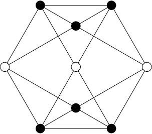
Refer to caption
Figure 6: A 44-regular graph which produces two hypergroup structures
Refer to caption
Figure 7: The line graph of 𝒫3\mathcal{P}_{3}
  • (iii)\mathrm{(iii)}

    Complete bipartite graphs

Let mm, n∈ℕn\in\mathbb{N} with mm, n≥2n\geq 2. The complete bipartite graph Km,n=(Vm,n,Em,n)K_{m,n}=(V_{m,n},E_{m,n}) is defined as follows:

  • •

    Vm,n={u1,u2,⋯,um,w1,w2,⋯,wn}V_{m,n}=\left\{u_{1},u_{2},\cdots,u_{m},w_{1},w_{2},\cdots,w_{n}\right\} (|Vm,n|=m+n\left\lvert V_{m,n}\right\rvert=m+n).

  • •

    Em,n={{uα,vβ}; 1≤α≤m,1≤β≤n}E_{m,n}=\left\{\left\{u_{\alpha},v_{\beta}\right\}\,;\,1\leq\alpha\leq m,1\leq\beta\leq n\right\}.

The complete bipartite graph Km,nK_{m,n} is of diameter two and is regular if and only if m=nm=n. We here meet an intriguing example, which is a non-regular hypergroup productive graph.

We can compute the structure identities of ℛ⁡(Km,n)\mathcal{R}(K_{m,n}) to be

R1∘v0R1=1m​R0+m−1m​R2,\displaystyle R_{1}\circ_{v_{0}}R_{1}=\frac{1}{m}R_{0}+\frac{m-1}{m}R_{2},
R1∘v0R2=R2∘v0R1=R1,\displaystyle R_{1}\circ_{v_{0}}R_{2}=R_{2}\circ_{v_{0}}R_{1}=R_{1},
R2∘v0R2=1m−1​R0+m−2m−1​R2\displaystyle R_{2}\circ_{v_{0}}R_{2}=\frac{1}{m-1}R_{0}+\frac{m-2}{m-1}R_{2}

if the base point v0v_{0} is chosen from uαu_{\alpha}’s and to be

R1∘v0R1=1n​R0+n−1n​R2,\displaystyle R_{1}\circ_{v_{0}}R_{1}=\frac{1}{n}R_{0}+\frac{n-1}{n}R_{2},
R1∘v0R2=R2∘v0R1=R1,\displaystyle R_{1}\circ_{v_{0}}R_{2}=R_{2}\circ_{v_{0}}R_{1}=R_{1},
R2∘v0R2=1n−1​R0+n−2n−1​R2\displaystyle R_{2}\circ_{v_{0}}R_{2}=\frac{1}{n-1}R_{0}+\frac{n-2}{n-1}R_{2}

if the base point v0v_{0} is chosen from vβv_{\beta}’s. Needless to say, these identities completely coincide when m=nm=n.

  • (iv)\mathrm{(iv)}

    Infinite ladder graph

Here will be introduced an example of infinite hypergroup productive graphs, which can be drawn like a ladder as in Figure 8. More precisely, we consider the Cayley graph ℒ=Cay⁡(ℤ⊕(ℤ/2​ℤ),{(±1,0¯),(0,1¯)})\mathcal{L}=\mathrm{Cay}\left(\mathbb{Z}\oplus\left(\mathbb{Z}/2\mathbb{Z}\right),\left\{(\pm 1,\overline{0}),(0,\overline{1})\right\}\right) in this part. (As mentioned in Theorem 1.1, 0¯\overline{0} and 1¯\overline{1} denote the residue classes of 00 and 11 modulo 22, respectively.) Since Cayley graphs are vertex-transitive, Proposition 4.2 allows one to assume that v0=(0,0¯)v_{0}=(0,\overline{0}) is the base point. The structure identities of ℛ⁡(ℒ)\mathcal{R}(\mathcal{L}) can be computed to be

R1∘R1=13​R0+23​R2,\displaystyle R_{1}\circ R_{1}=\frac{1}{3}R_{0}+\frac{2}{3}R_{2},
R1∘Ri=Ri∘R1=12​Ri−1+12​Ri+1(i≥2),\displaystyle R_{1}\circ R_{i}=R_{i}\circ R_{1}=\frac{1}{2}R_{i-1}+\frac{1}{2}R_{i+1}\quad(i\geq 2),
Ri∘Ri=14​R0+14​R2+18​R2​i−2+38​R2​i(i≥2),\displaystyle R_{i}\circ R_{i}=\frac{1}{4}R_{0}+\frac{1}{4}R_{2}+\frac{1}{8}R_{2i-2}+\frac{3}{8}R_{2i}\quad(i\geq 2),
Ri∘Rj=38​R|i−j|+18​R|i−j|+2+18​Ri+j−2+38​Ri+j(i,j≥2,i≠j).\displaystyle R_{i}\circ R_{j}=\frac{3}{8}R_{\left\lvert i-j\right\rvert}+\frac{1}{8}R_{\left\lvert i-j\right\rvert+2}+\frac{1}{8}R_{i+j-2}+\frac{3}{8}R_{i+j}\quad(i,j\geq 2,\,i\neq j).

To prove the claim (b)\mathrm{(b)} of Theorem 1.1, the associativity remains to be checked. It can be shown by elementary calculations (and Proposition 4.4).

Refer to caption
Figure 8: Infinite ladder graph
Remark.

One can find that the Cayley graph Cay⁡(ℤ⊕(ℤ/n​ℤ),{(±1,0¯),(0,±1¯)})\mathrm{Cay}\left(\mathbb{Z}\oplus\left(\mathbb{Z}/n\mathbb{Z}\right),\left\{(\pm 1,\overline{0}),(0,\overline{\pm 1})\right\}\right) admits no hypergroup productive pairs when n≥3n\geq 3. In addition, it turns out that the Cayley graph Cay⁡(ℤ⊕ℤ,{(±1,0),(0,±1)})\mathrm{Cay}\left(\mathbb{Z}\oplus\mathbb{Z},\left\{(\pm 1,0),(0,\pm 1)\right\}\right), which is actually expected to be hypergroup productive, also admits no hypergroup productive pairs. (This graph can be drawn as the square lattice in the Euclidean plane.) There is no known examples of graphs that admit a hypergroup productive pair but fail to be hypergroup productive graphs.

Remark.

Hypergroups derived from a random walk on an infinite graph can be realized as polynomial hypergroups since supp⁡(R1∘Ri)⊂{i−1,i,i+1}\mathrm{supp}\left(R_{1}\circ R_{i}\right)\subset\left\{i-1,i,i+1\right\}.

In particular, the hypergroup derived from a random walk on 𝒯2\mathcal{T}_{2} coincides with the hypergroup which can be constructed by the Chebyshev polynomials of the first kind, so that the hypergroup ℛ⁡(𝒯2)\mathcal{R}(\mathcal{T}_{2}) is called the Chebyshev hypergroup of the first kind. Tsurii [12] elucidated several properties of the Chebyshev hypergroup of the first kind. (He also investigate the Chebyshev hypergroup of the second kind in [12].)

For details of the polynomial hypergroups, see [3, Chapter 3] or [8] for example.

Acknowledgments.

The authors express their gratitude to Prof. Satoshi Kawakami, Prof. Kohji Matsumoto, Prof. Tatsuya Tsurii, Prof. Shigeru Yamagami and Mr. Ippei Mimura for helpful comments.

References

  • [1] R. A. Bailey, Association schemes: Designed experiments, algebra and combinatorics, Cambridge Univ. Press, 2004.
  • [2] N. Biggs, Algebraic graph theory (second edition), Cambridge Univ. Press, 1993.
  • [3] W. R. Bloom and H. Heyer, Harmonic analysis of probability measures on hypergroups, Walter de Gruyter & Co., 1995.
  • [4] A. E. Brouwer, A. M. Cohen and A. Neumaier, Distance-regular graphs, Springer-Verlag, 1989.
  • [5] C. F. Dunkl, The measure algebra of a locally compact hypergroup, Trans. Amer. Math. Soc. 179 (1973), 331–348.
  • [6] R. I. Jewett, Spaces with an abstract convolution of measures, Adv. in Math. (Springer) 18 (1) (1975), 1–101.
  • [7] S. Kawakami, T. Tsurii and S. Yamanaka, Deformations of finite hypergroups, Sci. Math. Jpn. (in Editione Electronica) 28 (2015), 2015-21 (published online).
  • [8] R. Lasser, Orthogonal polynomials and hypergroups, Rend. Mat. Appl. (7) 3 (1983), 185–209.
  • [9] Y. Matsuzawa, H. Ohno, A. Suzuki, T. Tsurii and S. Yamanaka, Non-commutative hypergroup of order five, J. Algebra Appl., to appear.
  • [10] W. Rudin, Functional analysis (second edition), McGraw-Hill Inc., 1991.
  • [11] R. Spector, Mesures invariantes sur les hypergroupes, Trans. Amer. Math. Soc. 239 (1978), 147–165.
  • [12] T. Tsurii, Deformations of the Chebyshev hypergroups, Sci. Math. Jpn. (in Editione Electronica) 28 (2015), 2015-54 (published online).
  • [13] N. J. Wildberger, Hypergroups associated to random walks on Platonic solids, Preprint, Univ. of NSW, 1994.
  • [14] N. J. Wildberger, Finite commutative hypergroups and applications from group theory to conformal field theory, Contemp. Math. 183 (1995), 413–434.
  • [15] N. J. Wildberger, Strong hypergroups of order three, J. of Pure Appl. Algebra 174 (1) (2002), 95–115.