Parameterized Complexity of the List Coloring Reconfiguration Problem with Graph ParametersThanks: This work is partially supported by JST CREST Grant Number JPMJCR1402, and by JSPS KAKENHI Grant Numbers JP16J02175, JP16K00003, and JP16K00004.
Abstract
Let be a graph such that each vertex has its list of available colors, and assume that each list is a subset of the common set consisting of colors. For two given list colorings of , we study the problem of transforming one into the other by changing only one vertex color assignment at a time, while at all times maintaining a list coloring. This problem is known to be PSPACE-complete even for bounded bandwidth graphs and a fixed constant . In this paper, we study the fixed-parameter tractability of the problem when parameterized by several graph parameters. We first give a fixed-parameter algorithm for the problem when parameterized by and the modular-width of an input graph. We next give a fixed-parameter algorithm for the shortest variant when parameterized by and the size of a minimum vertex cover of an input graph. As corollaries, we show that the problem for cographs and the shortest variant for split graphs are fixed-parameter tractable even when only is taken as a parameter. On the other hand, we prove that the problem is W[1]-hard when parameterized only by the size of a minimum vertex cover of an input graph.
1 Introduction
Recently, the framework of reconfiguration [16] has been extensively studied in the field of theoretical computer science. This framework models several situations where we wish to find a step-by-step transformation between two feasible solutions of a combinatorial (search) problem such that all intermediate solutions are also feasible and each step respects a fixed reconfiguration rule. This reconfiguration framework has been applied to several well-studied combinatorial problems. (See a survey [15].)
1.1 Our problem
In this paper, we study a reconfiguration problem for list (vertex) colorings in a graph, which was introduced by Bonsma and Cereceda [2].
Let be the set of colors, called the color set. A (proper) -coloring of a graph is a mapping such that for every edge . In list coloring, each vertex has a set of colors, called the list of ; sometimes, the list assignment itself is called a list. Then, a -coloring of is called an -coloring of if holds for every vertex . Therefore, a -coloring of is simply an -coloring of when holds for every vertex of , and hence -coloring is a generalization of -coloring. Figure 1(b) illustrates four -colorings of the same graph in Figure 1(a); the color assigned to each vertex is attached to the vertex.
In the reconfiguration framework, two -colorings and of a graph are said to be adjacent if holds, that is, can be obtained from by recoloring exactly one vertex. A sequence of -colorings of is called a reconfiguration sequence between and (of length ) if and are adjacent for each . Two -colorings and are reconfigurable if there exists a reconfiguration sequence between them. The list coloring reconfiguration problem is to determine whether two given -colorings and are reconfigurable, or not. Figure 1 shows an example of a yes-instance of list coloring reconfiguration, where the vertex whose color assignment was changed from the previous one is depicted by a black circle.

1.2 Known and related results
List coloring reconfiguration is one of the most well-studied reconfiguration problems, as well as coloring reconfiguration which is a special case of the problem such that holds for every vertex . These problems have been studied intensively from various viewpoints [1, 2, 3, 4, 7, 8, 14, 17, 20] including the generalizations [6, 21].
Bonsma and Cereceda [2] proved that coloring reconfiguration is PSPACE-complete even for bipartite graphs and any fixed constant . On the other hand, Cereceda et al. [8] gave a polynomial-time algorithm solving coloring reconfiguration for any graph and ; the algorithm can be applied to list coloring reconfiguration, too. In particular, the former result implies that there is no fixed-parameter algorithm for coloring reconfiguration (and hence list coloring reconfiguration) when parameterized by only under the assumption of .
Bonsma et al. [4] and Johnson et al. [17] independently developed a fixed-parameter algorithm to solve coloring reconfiguration when parameterized by , where is the upper bound on the length of reconfiguration sequences, and again their algorithms can be applied to list coloring reconfiguration. In contrast, if coloring reconfiguration is parameterized only by , then it is W[1]-hard when is an input [4] and does not admit a polynomial kernelization when is fixed unless the polynomial hierarchy collapses [17].
Hatanaka et al. [14] proved that list coloring reconfiguration is PSPACE-complete even for complete split graphs, whose modular-width is zero. Wrochna [20] proved that list coloring reconfiguration is PSPACE-complete even when and the bandwidth of an input graph are bounded by some constant; thus the treewidth and the cliquewidth of an input graph are also bounded.

1.3 Our contribution
To the best of our knowledge, known algorithmic results mostly employed the length of reconfiguration sequences as a parameter [4, 17], and no fixed-parameter algorithm is known when parameterized by graph parameters. Therefore, we study list coloring reconfiguration when parameterized by several graph parameters, and paint an interesting map of graph parameters which shows the boundary between fixed-parameter tractability and intractability. Our map is Figure 2 which shows both known and our results, where an arrow indicates that the parameter is “stronger” than , that is, is bounded if is bounded. (For relationships of parameters, see, e.g., [11, 18].)
More specifically, we first give a fixed-parameter algorithm solving list coloring reconfiguration when parameterized by and the modular-width of an input graph. (The definition of modular-width will be given in Section 2.1.) Note that, according to the known results [2, 14], we cannot construct a fixed-parameter algorithm for general graphs when only one of and is taken as a parameter under the assumption of . However, as later shown in Corollary 1, our algorithm implies that the problem is fixed-parameter tractable for cographs even when only is taken as a parameter.
We then consider the shortest variant which computes the length of a shortest reconfiguration sequence (i.e., the minimum number of recoloring steps) for a yes-instance of list coloring reconfiguration, and show that it admits a fixed-parameter algorithm when parameterized by and the size of a minimum vertex cover of an input graph. Moreover, as a corollary, we show that the shortest variant is fixed-parameter tractable for split graphs even when only is taken as a parameter.
Finally, we prove that list coloring reconfiguration is -hard when parameterized only by the size of a minimum vertex cover of an input graph.
2 Preliminaries
We assume without loss of generality that graphs are simple and connected. Let be a graph with vertex set and edge set ; we sometimes denote by and the vertex set and the edge set of , respectively. For a vertex in , we denote by the neighborhood of in . For a vertex subset , we denote by the subgraph of induced by , and denote . For a subgraph of , we denote . Let be the size of a maximum clique of . We have the following simple observation.
Observation 1
Let be a graph with a list . If has an -coloring, then .
A graph is split if its vertex set can be partitioned into a clique and an independent set. A graph is a cograph (or a -free graph) if it contains no induced path with four vertices.
2.1 Modules and modular decomposition


A module of a graph is a vertex subset such that for every two vertices and in . In other words, the module is the set of vertices whose neighborhoods in are the same. For example, the graph in Figure 3(a) has a module for which holds. Note that the vertex set of , the set consisting of only a single vertex, and the empty set are all modules of ; they are called trivial. A graph is a prime if all of its modules are trivial; for an example, see Figure 3(b).

We now introduce the notion of modular decomposition, which was first presented by Gallai in 1967 as a graph decomposition technique [12]. For a survey, see, e.g., [13].
We first define the substitution operation, which constructs one graph from more than one graphs. Let be a graph, called a quotient graph, consisting of nodes , and let be a family of vertex-disjoint graphs such that corresponds to for every . The -substitution of , denoted by , is the graph which is obtained by taking a union of all graphs in and then connecting every pair of vertices and by an edge if and only if and are adjacent in . That is, the vertex set of is , and the edge set of is the union of and . (See Figure 4 as an example.)
A substitution tree is a rooted tree such that each non-leaf node is associated with a quotient graph and has child nodes. For each node , we can recursively define the corresponding graph as follows: If is a leaf, consists of a single vertex. Otherwise, let be children of , then . For the root of , is called the corresponding graph of , and we denote . We say that is a substitution tree for a graph if , and refer to a node in in order to distinguish it from a vertex in . Figure 5(a) illustrates a substitution tree for the graph in Figure 5(b); each leaf , , corresponds to the subgraph of consisting of a single vertex . We note that the vertex set of each corresponding graph , , forms a module of .
A modular decomposition tree (an MD-tree for short) for a graph is a substitution tree for which satisfies the following three conditions:
- •
Each node applies to one of the following three types:
- –
a series node, whose quotient graph is a complete graph;
- –
a parallel node, whose quotient graph is an edge-less graph; and
- –
a prime node, whose quotient graph is a prime with at least four vertices.
- –
- •
No edge connects two series nodes.
- •
No edge connects two parallel nodes.
It is known that any graph has a unique MD-tree with nodes, and it can be computed in time [19]. We denote by the unique MD-tree for a graph . The modular-width of a graph is the maximum number of children of a prime node in its MD-tree . The substitution tree in Figure 5(a) is indeed the MD-tree for the graph in Figure 5(b), and hence ; note that only is a prime node in .
We now define a variant of MD-trees, which will make our proofs and analyses simpler. A pseudo modular decomposition tree (a PMD-tree for short) for a graph is a substitution tree for which satisfies the following two conditions:
- •
Each node applies to one of the following three types:
- –
a -join node, whose quotient graph is a complete graph with exactly two vertices;
- –
a parallel node, whose quotient graph is an edge-less graph; and
- –
a prime node, whose quotient graph is a prime with at least four vertices.
- –
- •
No edge connects two parallel nodes.
Proposition 1
For any graph , there exists a PMD-tree with nodes such that each prime node has at most children, and it can be constructed in polynomial time.
Proof
Recall that an MD-tree for a graph can be constructed in linear time. Given an MD-tree for a graph , we thus construct a PMD-tree such that as follows. For each series node of having children , we replace it with a binary tree consisting of nodes such that has two children and for each and has two children and . A quotient graph of each new node is defined as a complete graph with exactly two vertices. Then, is a PMD-tree for , it has at most nodes, and each prime node has at most children. Moreover, this process can be done in time polynomial in . ∎
We denote by a substitution tree for such that each prime node has at most children. The pseudo modular-width of a graph is the maximum number of children of a non-parallel node in its PMD-tree. Notice that holds.
2.2 Other notation
Let be a graph, and let be a list. For two -colorings and of a graph , we define the difference between and as the set . Notice that and are adjacent if and only if .
We express an instance of list coloring reconfiguration by a -tuple consisting of a graph , a list , and initial and target -colorings and of .
Finally, we introduce a notion of “restriction” of mappings and instances. Consider an arbitrary mapping , where is a graph and is any set. For a subgraph of , we denote by the restriction of on , that is, is a mapping from to such that for each vertex . Let be an instance of list coloring reconfiguration. For a subgraph of , we define the restriction of (on ) as the instance of list coloring reconfiguration. Notice that and are proper -colorings of .
3 Fixed-Parameter Algorithm for Bounded Modular-Width Graphs
The following is our main theorem of this section.
Theorem 3.1
List coloring reconfiguration is fixed-parameter tractable when parameterized by , where and are the upper bounds on the size of the color set and the modular-width of an input graph, respectively.
Because it is known that any cograph has modular-width zero, we have the following result as a corollary of Theorem 3.1.
Corollary 1
List coloring reconfiguration is fixed-parameter tractable for cographs when parameterized by the size of the color set.
Recall that , and hence . Therefore, as a proof of Theorem 3.1, it suffices to give a fixed-parameter algorithm for list coloring reconfiguration with respect to , where is an upper bound on .
3.1 Reduction rule

In this subsection, we give a useful lemma, which compresses an input graph into a smaller graph with keeping the reconfigurability.
Let be an instance of list coloring reconfiguration. For each vertex , we define a vertex assignment as a triple consisting of a list, and initial and target color assignments of . Let and be two induced subgraphs of such that and Then, and are identical (on ) if there exists a bijective function which satisfies all the following two conditions:
- 1.
and are isomorphic under , that is, if and only if .
- 2.
For all vertices ,
- (a)
; and
- (b)
, that is, , and .
- (a)
We note that the condition 2(a) implies that there is no edge between and . Figure 6 shows an example of identical subgraphs and on , where the bijective function maps each vertex in to a vertex in with the same shape.
We now prove the following key lemma, which holds for any graph.
Lemma 1
(Reduction rule) Let be an instance of list coloring reconfiguration, and let and be two identical subgraphs of . Then, is a yes-instance if and only if is.
Proof
We assume that and are identical under a bijective function , and let .
We first prove the if direction. Suppose that is a yes-instance. Then, there exists a reconfiguration sequence for , where . For each , since is an -coloring of , is an -coloring of . Therefore, by removing all consecutive duplicate -colorings, is a reconfiguration sequence for . Thus is a yes-instance.
We now prove the only-if direction. Suppose that is a yes-instance. Then, there exists a reconfiguration sequence for with and . Our goal is to construct a reconfiguration sequence for from . For each , we first extend to as follows:
We claim that is a proper -coloring of . To show this, it suffices to check that holds for each and its neighbors . If , holds because and is an -coloring. Otherwise, holds because and is an -coloring. Therefore, the obtained sequence consists only of -colorings of . However, there may exist several indices such that and are not adjacent, because may hold. Recall that and are adjacent for each , that is, for some vertex . If , holds, and hence and are adjacent. Otherwise, holds, and hence and are not adjacent. In this case, between and , we insert an -coloring of defined as follows:
Observe that is a proper -coloring of . Moreover, both and hold. Thus, we obtain a proper reconfiguration sequence for as claimed. ∎
3.2 Kernelization
Let be an instance of list coloring reconfiguration. Suppose that the color set has at most colors, is a connected graph with , and all vertices of are totally ordered according to an arbitrary binary relation .
Sufficient condition for identical subgraphs.
We first give a sufficient condition for which two nodes in a PMD-tree for correspond to identical subgraphs. Let be a node, let , and assume that all vertices in are labeled as according to ; that is, holds for each with . Let be some integer which will be defined later. We now define an matrix as follows:
where denotes an -element of . Notice that contains an adjacency matrix of at its upper left submatrix, and the bottommost row represents the vertex assignment of each vertex in . We call an -ID-matrix of . For example, consider the node in Figure 5(a). Then, , and a -ID-matrix of is as follows:
Lemma 2
Let and be two children of a parallel node in , and let be an integer with . If holds, then and are identical.
Proof
Let and . Observe that if and only if , and if and only if . By the assumption that for all , we have ; we denote by this value.
We now check that and are identical. The condition 1 of identical subgraphs holds, because the upper left submatrices in and correspond to the adjacency matrices of and , respectively. The condition 2(b) holds, because the bottommost rows are the same in and . Finally, we claim that the condition 2(a) holds, as follows. Since is a parallel node, holds for all vertices in . Similarly, holds for all vertices in . Recall that is a module of , that is, holds for any vertice . Therefore, holds any pair of and . Thus, the condition 2(a) holds. ∎
Kernelization algorithm.
We now describe how to kernelze an input instance. (See Figure 7 as an example.) Our algorithm traverses a PMD-tree of by a depth-first search in post-order starting from the root of , that is, the algorithm processes a node of after its all children are processed.
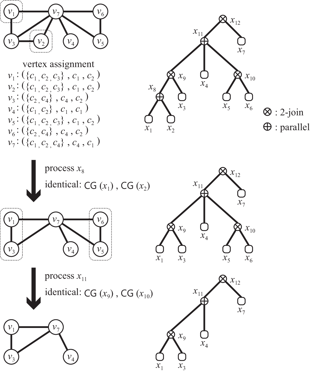
Let be a node which is currently visited. If is a non-parallel node, we do nothing. Otherwise (i.e., if is a parallel node,) let be the set of all children of , and let . We first construct -ID-matrices of all children of . If there exist two nodes and such that , then and are identical; and hence we remove from by Lemma 1. Then, we modify in order to keep it still being a PMD-tree for the resulting graph as follows. We remove a subtree rooted at from , and delete a node corresponding to from a quotient graph of . If this removal makes having only one child in the PMD-tree, we contract the edge into a new node such that .
The running time of this kernelization can be estimated as follows. For each node , the construction of -ID-matrices can be done in time . We can check if for each pair of children and of in time . Moreover, a modification of , which follows an application of Lemma 1, can be done in polynomial time. Recall that the number of children of and the size of a PMD-tree are both bounded linearly in , and hence our kernelization can be done in polynomial time.
Size of the kernelized instance.
We finally prove that the size of the obtained instance depends only on ; recall that is the upper bound on . By Observation 1, we can assume that the maximum clique size is at most . In addition, is connected since is connected and an application of Lemma 1 does not affect the connectivity of the graph. Therefore, it suffices to prove the following lemma.
Lemma 3
The graph has at most vertices, where is recursively defined for an integer as follows:
In particuler, depends only on .
Proof
We prove the lemma by induction on . If , then we have since is connected.
We thus assume in the remainder of the proof that . Then, the root of a PMD-tree for must be a non-parallel node since is connected. Because has at most children, it suffices to show that the corresponding graph of each child of has at most
vertices. We will prove this by showing the following two claims for any child of :
- (A)
holds for any connected component of ; and
- (B)
has at most connected components.
In order to prove the claim (A), we first claim that holds. Assume for a contradiction that contains a clique of size . Let be a node of a quotient graph which corresponds to . By the definition, is connected, and hence there exists a node which is adjacent to . Let be the child of corresponding to . Recall that all vertices in are connected with at least one vertex in by the substitution operation, which means that has a clique of size . This contradicts the assumption that the maximum clique size of is ; this completes the proof of the claim. Note that holds for any connected component of . Therefore, follows from the induction hypothesis.
We next prove the claim (B). If is a non-parallel node, is connected and hence we are done. The remaining case is where is a parallel node. Let be a connected component of , and let be the set of all children of . Then, there exists exactly one child such that . Since a PMD-tree has no edge joining two parallel nodes, is not a parallel node. Thus, is connected, and hence we indeed have . Therefore, it suffices to bound the size of instead of the number of connected components in . Let . Since is already kernelized, holds for any two children . Therefore, cannot exceed the number of distinct -ID-matrices. Recall that the upper submatrix consists of values from , its -element is for each , and it is symmetric. Therefore, the number of such submatrices can be bounded by . Recall that all elements of the -st row are chosen from the set , where is the color set of size at most . Therefore, the number of such submatrices can be bounded by . By the claim (A), we have . Therefore, the size of , and hence the number of connected components in , can be bounded by
From the claims (A) and (B), we have the following inequality.
as claimed. In particular, we can conclude that depends only on , because . ∎
Finally, we prove Theorem 3.1. By the above discussions, we can compute the kernelized instance of list coloring reconfiguration in polynomial time. Because the size of depends only on , we can solve by enumerating all -colorings. The running time for this enumeration depends only on , and hence we obtain a fixed-parameter algorithm for list coloring reconfiguration.
This completes the proof of Theorem 3.1.
4 Shortest Variant
In this section, we study the shortest variant, list coloring shortest reconfiguration. We note that the shortest length can be expressed by a polynomial number of bits, because there are at most colorings for a graph with vertices and colors. Therefore, the answer can be output in polynomial time. The following is our result.
Theorem 4.1
List coloring shortest reconfiguration is fixed-parameter tractable when parameterized by , where and are the upper bounds on the sizes of the color set and a minimum vertex cover of an input graph, respectively.
As a corollary, we have the following result.
Corollary 2
List coloring shortest reconfiguration is fixed-parameter tractable for split graphs when parameterized by the size of the color set.
Proof
Let be an instance of list coloring shortest reconfiguration such that is a split graph. Assume that the vertex set of can be partitioned into a clique and an independent set . By Observation 1, we have . Observe that forms a vertex cover of . Thus, holds for split graphs. ∎
As a proof of Theorem 4.1, we give such a fixed-parameter algorithm. Our basic idea is the same as the fixed-parameter algorithm in Section 3. However, in order to compute the shortest length, we consider a more general “weighted” version of list coloring shortest reconfiguration, which is defined as follows. Let be an instance of list coloring reconfiguration, and assume that each vertex has a weight , where is the set of all positive integers. For two adjacent -colorings and of a graph , we define the gap between and as the weight of , where is a unique vertex in . The length of a reconfiguration sequence is defined as . We denote by the length of a shortest reconfiguration sequence between and ; we define if is a no-instance of list coloring reconfiguration. Then, list coloring shortest reconfiguration can be seen as computing for the case where every vertex has weight one. Thus, to prove Theorem 4.1, it suffices to construct a fixed-parameter algorithm for the weighted version when parameterized by .
As with Section 3, we again use the concept of kernelization to prove Theorem 4.1. More precisely, for a given instance , we first construct an instance in polynomial time such that the size of depends only on , and holds. Then, we can compute by computing a (weighted) shortest path between and in an edge-weighted graph defined as follows: the vertex set consists of all -colorings of , and each pair of adjacent -colorings are connected by an edge with a weight corresponding to the gap between them.
4.1 Reduction rule for the weighted version

In this subsection, we give the counterpart of Lemma 1 for the weighted version.
We first introduce some notation. Let be a reconfiguration sequence for an instance of list coloring reconfiguration. For each vertex , we denote by the number of indices such that . In other words, is the number of steps recoloring in . Notice that holds for any weight function .
Let be an instance of the weighted version, and assume that there exist two identical subgraphs and of , both of which consist of single vertices, say, and . We now define a new instance as follows (see also Figure 8):
- •
; and
- •
and for any .
Intuitively, is merged into together with its weight. Then, we have the following lemma.
Lemma 4
.
Proof
For the notational convenience, we denote . By Lemma 1, if and only if . Therefore, we assume that and .
We first show that . Since holds for any reconfiguration sequence for , it suffices to show that there exists a reconfiguration sequence for whose length is at most . Let be a shortest reconfiguration sequence for such that . Following the only-if direction proof of Lemma 1, we can construct a reconfiguration sequence for such that and for any . Therefore,
Thus, is a desired reconfiguration sequence for .
We next show that . Since holds for any reconfiguration sequence for , it suffices to show that there exists a reconfiguration sequence for whose length is at most . Let be a shortest reconfiguration sequence for such that . We now construct a reconfiguration sequence for from such that as follows.
- Case 1. :
-
In this case, we restrict all -colorings in on to obtain a reconfiguration sequence for ; recall the if direction proof of Lemma 1. From the construction, and holds for any vertex . Therefore, we have
Thus, is a desired reconfiguration sequence for .
- Case 2. :
-
In this case, instead of restricting -colorings in on , we restrict them on and obtain a reconfiguration sequence for . Then, because and are identical, we can easily “rephrase” as a reconfiguration sequence for . By the same arguments as the case 1 above, we have . Thus, is a desired reconfiguration sequence for .
In this way, we have shown that as claimed. ∎
4.2 Kernelazation
Finally, we give a kernelization algorithm as follows.
Let be an instance of the weighted version such that has a vertex cover of size at most . Because such a vertex cover can be computed in time [9], we now assume that we are given a vertex cover of size at most . Notice that forms an independent set of . Suppose that there exist two vertices such that and hold. Then, induced subgraphs and are identical. Therefore, we can apply Lemma 4 to remove from , and modify a weight function without changing the optimality. As a kernelization, we repeatedly apply Lemma 4 for all such pairs of vertices in , which can be done in polynomial time. Let be the resulting subgraph of , and let . Since is of size at most , it suffices to prove the following lemma.
Lemma 5
.
Proof
Recall that contains no pair of vertices which induce identical subgraphs, and hence any pair of vertices does not satisfy at least one of and . Therefore, can be bounded by the number of distinct combinations of the neighborhood and the vertex assignment. Since is an independent set, for each vertex . Recall that , and hence the number of (possible) neighborhoods can be bounded by . Since there are at most colors, the number of (possible) vertex assignments can be bounded by . We thus have as claimed. ∎
This completes the proof of Theorem 4.1.
5 W[1]-hardness
Because even the shortest variant is fixed-parameter tractable when parameterized by , one may expect that is a strong parameter and the problem is fixed-parameter tractable with only . However, we prove the following theorem in this section.
Theorem 5.1
List coloring reconfiguration is -hard when parameterized by , where is the upper bound on the size of a minimum vertex cover of an input graph.
Recall that list coloring reconfiguration is PSPACE-complete even for a fixed constant . Therefore, the problem is intractable if we take only one parameter, either or .
In order to prove Theorem 5.1, we give an FPT-reduction from the independent set problem when parameterized by the solution size , in which we are given a graph and an integer , and asked whether has an independent set of size at least . This problem is known to be W[1]-hard [9].
5.1 Construction
Let be a graph with vertices , and be an integer as an input for independent set. Then, we construct the corresponding instance of list coloring reconfiguration as follows. (See also Figure 9.)

We first create vertices , which are called selection vertices; let be the set of all selection vertices. For each , we set . In our reduction, we will construct and so that assigning the color , , to corresponds to choosing the vertex as a vertex in an independent set of . Then, in order to make a correspondence between a color assignment to and an independent set of size in , we need to construct the following properties:
- •
For each , we use at most one color from ; this ensures that each vertex can be chosen at most once as an independent set.
- •
For each with , we use at most one color from ; then, no two adjacent vertices in are chosen as an independent set.
To do this, we define an -forbidding gadget for and . The -forbidding gadget is a vertex which is adjacent to and and has a list . Observe that the vertex forbids that and are simultaneously colored with and , respectively. In order to satisfy the desired properties above, we now add our gadgets as follows: for all with ,
- •
add an -forbidding gadget for every vertex ; and
- •
add - and -forbidding gadgets for every edge .
We denote by the set of all vertices in the forbidding gadgets. We finally create an edge consisting of two vertices and such that and , and connect with all selection vertices in .
Finally, we construct two -colorings and of as follows:
- •
for each , ;
- •
for each , and are arbitrary chosen colors from ; and
- •
, and .
Note that both and are proper -colorings of .
In this way, we complete the construction of .
5.2 Correctness of the reduction
In this subsection, we prove the following three statements:
- •
can be constructed in time polynomial in the size of .
- •
The upper bound on the size of a minimum vertex cover of depends only on .
- •
is a yes-instance of independent set if and only if is a yes-instance of list coloring reconfiguration.
In order to prove the first statement, it suffices to show that the size of is bounded polynomially in . From the construction, we have . In addition, each list contains colors. Therefore, the construction can be done in time .
The second statement immediately follows from the fact that is a vertex cover in of size ; observe that contains no edge.
Finally, we prove the last statement as follows.
Lemma 6
is a yes-instance of independent set if and only if is a yes-instance of list coloring reconfiguration.
Proof
We first prove the if direction. Assume that there exists a reconfiguration sequence for . Then, must contain at least one -coloring such that in order to recolor from to . Since is adjacent to all vertices in , holds for every . Then, by the construction, the vertex set is an independent set in of size .
We then prove the only-if direction. We construct a reconfiguration sequence for which passes through two -colorings and defined as follows.
From the assumption, has an independent set of size , say, . Then, we define as follows:
- •
for each , ;
- •
for each -forbidding vertex , is an arbitrary chosen color from ; and
- •
and .
Note that is a proper -coloring of . We next show that and are reconfigurable. We first recolor all vertice to the colors in an arbitrary order. This can be done, since for all and is an independent set in . We then recolor all vertices to the colors in an arbitrary order. This also can be done, since is a proper -coloring and is an independent set in . Thus, and are reconfigurable.
By the similar arguments as , we define as follows:
- •
for each , ;
- •
for each -forbidding vertex , is an arbitrary chosen color from ; and
- •
and .
Then, and are reconfigurable.
Finally, we prove that and are reconfigurable. Recall that , , and for all . Then, we can swap the color and by the following three steps:
- •
recolor to ;
- •
recolor to ; and
- •
recolor to .
After that, we can recolor all vertices to the colors in the arbitrary order, since is an independent in
Therefore, is a yes-instance of list coloring reconfiguration. ∎
This completes the proof of Theorem 5.1.
6 Conclusion
In this paper, we have studied list coloring reconfiguration from the viewpoint of parametrized complexity, in particular, with several graph parameters, and painted an interesting map of graph parameters in Figure 2 which shows the boundary between fixed-parameter tractability and intractability.
References
- [1] Bonamy, M., Bousquet, N.: Recoloring bounded treewidth graphs. Electronic Notes in Discrete Mathematics 44, pp. 257–262 (2013)
- [2] Bonsma, P., Cereceda, L.: Finding paths between graph colourings: PSPACE-completeness and superpolynomial distances. Theoretical Computer Science 410, pp. 5215–5226 (2009)
- [3] Bonamy, M., Johnson, M., Lignos, I., Patel, V., Paulusma, D.: Reconfiguration graphs for vertex colourings of chordal and chordal bipartite graphs. J. Combinatorial Optimization 27, pp. 132–143 (2014)
- [4] Bonsma, P., Mouawad, A.E., Nishimura, N., Raman, V.: The complexity of bounded length graph recoloring and CSP reconfiguration. Proc. of IPEC 2014, LNCS 8894, pp. 110–121 (2014)
- [5] Brandstädt, A., Le, V.B., Spinrad, J.P.: Graph Classes: A Survey. SIAM (1999)
- [6] Brewster, R.C., McGuinness, S., Moore, B., Noel, J.A.: A dichotomy theorem for circular colouring reconfiguration. Theoretical Computer Science 639, pp. 1–13 (2016)
- [7] Cereceda, L.: Mixing Graph Colourings. Ph.D. Thesis, London School of Economics and Political Science (2007)
- [8] Cereceda, L., van den Heuvel, J., Johnson, M.: Finding paths between -colorings. J. Graph Theory 67, pp. 69–82 (2011)
- [9] Downey, R., G., Fellows, M., R.: Parameterized Complexity. Springer-Verlag New York (1999)
- [10] Dyer, M., Flaxman, A., Frieze, A., Vigoda, E.: Randomly colouring sparse random graphs with fewer colours than the maximum degree. Random Structures Algorithms 29, pp. 450–465 (2006)
- [11] Gajarský, J., Lampis, M., Ordyniak, S.: Parameterized algorithms for modular-width. Proc. of IPEC 2013, LNCS 8246, pp. 163–176 (2013)
- [12] Gallai, T.: Transitiv orientierbare Graphen. Acta Mathematica Academiae Scientiarum Hungarica 18, Issue 1-2, pp. 25–66 (1967)
- [13] Habib, M., Paul, C.: A survey of the algorithmic aspects of modular decomposition. Computer Science Review 4, issue 1, pp. 41–59 (2010)
- [14] Hatanaka, T., Ito, T., Zhou, X.: The list coloring reconfiguration problem for bounded pathwidth graphs. IEICE Trans. on Fundamentals of Electronics, Communications and Computer Sciences E98-A, No. 6, pp. 1168–1178 (2015)
- [15] van den Heuvel, J.: The complexity of change. Cambridge University Press, pp. 127–160 (2013)
- [16] Ito, T., Demaine, E.D., Harvey, N.J.A., Papadimitriou, C.H., Sideri, M., Uehara, R., Uno, Y.: On the complexity of reconfiguration problems. Theoretical Computer Science 412, pp. 1054–1065 (2011)
- [17] Johnson, M., Kratsch, D., Kratsch, S., Patel, V., Paulusma, D.: Finding shortest paths between graph colourings. Algorithmica 75, Issue 2, pp. 295–-321 (2016)
- [18] Kannan, S., Naor, M., Rudich, S.: Implicit representation of graphs. SIAM J. Discrete Mathematics 5, pp. 596–603 (1992)
- [19] McConnell, R.M., de Montgolfier, F.: Linear-time modular decomposition of directed graphs. Discrete Applied Mathematics 145, pp. 198–209 (2005)
- [20] Wrochna, M.: Reconfiguration in bounded bandwidth and treedepth. arXiv:1405.0847 (2014)
- [21] Wrochna, M.: Homomorphism reconfiguration via homotopy. Proc. of STACS 2015, LIPIcs 30, pp. 730–742 (2015)