On the Phase Transition of Corrupted SensingThanks: This work was supported by the National Natural Science Foundation of China under Grant 61301188.

Huan Zhang¹², Yulong Liu³, and Hong Lei¹ Affiliation: Affiliation: ¹Institute of Electronics, Chinese Academy of Sciences, Beijing 100190, China Affiliation: Affiliation: ²University of Chinese Academy of Sciences, Beijing 100049, China Affiliation: Affiliation: ³School of Physics, Beijing Institute of Technology, Beijing 100081, China Affiliation:

Abstract

In [1], a sharp phase transition has been numerically observed when a constrained convex procedure is used to solve the corrupted sensing problem. In this paper, we present a theoretical analysis for this phenomenon. Specifically, we establish the threshold below which this convex procedure fails to recover signal and corruption with high probability. Together with the work in [1], we prove that a sharp phase transition occurs around the sum of the squares of spherical Gaussian widths of two tangent cones. Numerical experiments are provided to demonstrate the correctness and sharpness of our results.

Index Terms:

Corrupted sensing, phase transition, Gaussian width, compressed sensing, signal separation.

I Introduction

Corrupted sensing aims to recover a structured signal from a small number of corrupted measurements

\bm{y}=\bm{\Psi}\bm{x}^{\star}+\bm{v}^{\star},

(1)

where $\bm{\Psi}\in\mathbb{R}^{m\times n}$ is the sensing measurement matrix which is assumed to have i.i.d. standard Gaussian entries in this paper, $\bm{x}^{\star}\in\mathbb{R}^{n}$ is the unknown signal, and $\bm{v}^{\star}\in\mathbb{R}^{m}$ is an unknown corruption. The goal is to estimate $\bm{x}^{\star}$ and $\bm{v}^{\star}$ from $\bm{y}$ and $\bm{\Psi}$ .

This problem is encountered in many practical applications, such as face recognition [2], subspace clustering[3], network data analysis [4], and so on. Theoretical guarantees for this problem include sparse signal recovery from sparse corruption [5, 6, 7, 8, 9, 10, 11] and structured signal recovery from structured corruption [1, 12, 13].

To make the recovery possible, we will assume that both $\bm{x}$ and $\bm{v}$ have some structures which are promoted by the convex functions $f(\cdot)$ and $g(\cdot)$ respectively. When prior information about $f(\bm{x}^{\star})$ or $g(\bm{v}^{\star})$ is available, it is natural to consider the following program to recover the signal and corruption:

\min f(\bm{x}),\quad\text{s.t. }\bm{y}=\bm{\Psi}\bm{x}+\bm{v},\quad g(\bm{v})\leq g(\bm{v}^{\star}),

(2)

\min g(\bm{v}),\quad\text{s.t. }\bm{y}=\bm{\Psi}\bm{x}+\bm{v},\quad f(\bm{x})\leq f(\bm{x}^{\star}).

(3)

In [1], Foygel and Mackey provided conditions under which convex program (2) or (3) succeeds with high probability. Numerical experiments in [1] also suggested that there is a sharp phase transition when (2) or (3) is used to solve the corrupted sensing problem. However, little work has devoted to determining the threshold below which (2) or (3) fails with high probability. Therefore, theoretical understanding of the phase transition for program (2) and (3) is far from satisfactory.

In this paper, we present a theoretical analysis for the phase transition of (2) or (3). In particular, we figure out the exact position of phase transition, and demonstrate that the phase transition occurs in a relatively narrow region.

II Preliminaries

In this section, we present some preliminaries which will be used in our analysis.

Our result involves two important concepts: the Gaussian width and the tangent cone. Given a subset $T$ in $\mathbb{R}^{n}$ , the Gaussian width is defined by

\omega(T)=\mathbb{E}\sup_{\bm{t}\in T}\left<\bm{g},\bm{t}\right>,\text{ where }\bm{g}\sim N(0,I_{n}).

We also define two tangent cones corresponding to signal and corruption respectively. The tangent cone of $f(\cdot)$ at the true signal $\bm{x}^{\star}$ is defined as

\mathcal{D}_{s}=\big\{\bm{a}\in\mathbb{R}^{n}:\exists~t>0,f(\bm{x}^{\star}+\bm{a}t)\leq f(\bm{x}^{\star})\big\}.

(4)

Similarly, the tangent cone of $g(\cdot)$ at the true corruption $\bm{v}^{\star}$ is given by

\mathcal{D}_{c}=\big\{\bm{b}\in\mathbb{R}^{m}:\exists~t>0,g(\bm{v}^{\star}+\bm{b}t)\leq g(\bm{v}^{\star})\big\}.

(5)

III Main results

In this section, we state our main results with some discussions.

Theorem 1 (Failure of convex program (2) or (3)).

Consider convex program (2) or (3). Assume that both tangent cones $\mathcal{D}_{s}$ and $\mathcal{D}_{c}$ are closed. For any $t\geq 0$ , if the measurement number $m$ satisfies

\sqrt{m}<\sqrt{\omega^{2}\big(\mathcal{D}_{s}\cap S^{n-1}\big)+\omega^{2}\big(\mathcal{D}_{c}\cap S^{m-1}\big)}-t,

then the constrained convex program (2) or (3) fails with probability at least $1-\exp(-t^{2}/2)$ , where $S^{n-1}$ and $S^{m-1}$ are the unit sphere of $\mathbb{R}^{n}$ and $\mathbb{R}^{m}$ respectively.

Proof.

See Appendix A. ∎

Remark 1 (Phase transition of corrupted sensing).

Recall Theorem $1$ and Remark $2$ in [1], which stated that ¹¹ 1 The authors believe that the small additive constants are artifacts of the proof technique.²² 2 The original result is stated in terms of Gaussian complexity $\gamma(\mathcal{D}_{s}\cap B^{n})$ , difined as $\gamma^{2}(\mathcal{D}_{s}\cap B^{n})=\mathbb{E}\big(\sup_{t\in\mathcal{D}_{s}\cap B^{n}}\left<g,t\right>\big)^{2}$ , where $B^{n}$ denotes the $\ell_{2}$ unit ball in $\mathbb{R}^{n}$ . However, as the author stated, the Gaussian complexity $\gamma(\mathcal{D}_{s}\cap B^{n})$ is only very slightly larger than $\omega(\mathcal{D}_{s}\cap S^{n-1})$ . when

\sqrt{m}\geq\sqrt{\omega^{2}(\mathcal{D}_{s}\cap S^{n-1})+\omega^{2}(\mathcal{D}_{c}\cap S^{m-1})}+\frac{1}{\sqrt{2}}+\frac{1}{\sqrt{2\pi}}+t,

the constrained convex program (2) or (3) succeeds with probability at least $1-\exp(-t^{2}/2)$ . This, together with our result Theorem 1, demonstrate that the phase transition of corrupted sensing occurs around

\omega^{2}\big(\mathcal{D}_{s}\cap S^{n-1}\big)+\omega^{2}\big(\mathcal{D}_{c}\cap S^{m-1}\big),

and the width of phase transition area is about

C\sqrt{\omega^{2}\big(\mathcal{D}_{s}\cap S^{n-1}\big)+\omega^{2}\big(\mathcal{D}_{c}\cap S^{m-1}\big)},

where $C$ is an absolute constant.

Remark 2.

Our result also agrees with the result of Amelunxen el al. [14]. Indeed, by Proposition 10.2 and Proposition 3.1 (9) in [14], we have

\omega^{2}\big(\mathcal{D}_{s}\cap S^{n-1}\big)+\omega^{2}\big(\mathcal{D}_{c}\cap S^{m-1}\big)\approx\delta(\mathcal{D}_{s})+\delta(\mathcal{D}_{c})=\delta(\mathcal{D}_{s}\times\mathcal{D}_{c}),

where $\delta(\mathcal{D})$ denotes the statistical dimension of a convex cone $\mathcal{D}$ .

Remark 3.

In [14], Amelunxen et al. considered the phase transition of the following demixing problem:

\bm{z}=\bm{x}+\bm{U}\bm{y},

where $\bm{x}$ , $\bm{y}\in\mathbb{R}^{n}$ are unknown signals and $\bm{U}\in\mathbb{R}^{n\times n}$ is a random orthogonal matrix. This model is different from ours since we have random Gaussian measurement matrix with $m\ll n$ .

Remark 4.

In [15], Oymak and Tropp considered the phase transition of the following demixing model:

\bm{y}=\bm{\Psi}_{0}\bm{x}_{0}+\bm{\Psi}_{1}\bm{x}_{1},

where $\bm{x}_{0}$ , $\bm{x}_{1}\in\mathbb{R}^{n}$ are two signals and $\bm{\Psi}_{0}$ , $\bm{\Psi}_{1}\in\mathbb{R}^{m\times n}$ are some random transformation matrices. This model is also different from ours since $\bm{\Psi}_{1}$ is a deterministic matrix in our case. This makes the problem more difficult to analyze.

IV Simulation Results

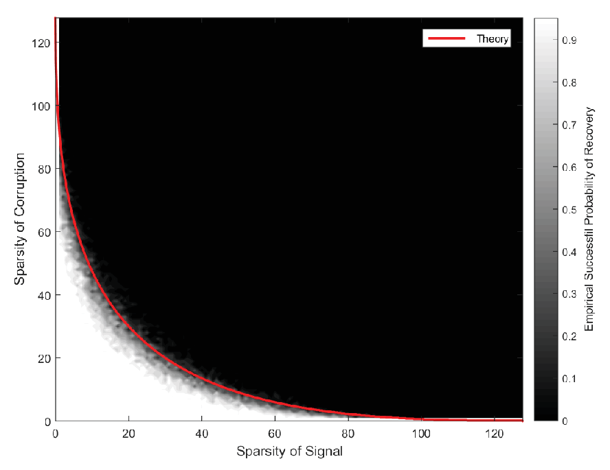
In this section, we employ a numerical experiment to verify our theoretical guarantees (Theorem 1). In the experiment, both signal and corruption are designed to be sparse vectors. We use CVX [16] [17] to solve the convex program (2) or (3).

In the experiment, we assume that the prior information of $f(\bm{x}^{\star})$ is known exactly, and solve program (3). The experiment settings are as follows: the ambient dimension $n$ is set to $128$ , the measurement number $m=n=128$ , the sparsity level of signal changes from $1$ to $n$ with step $1$ , and the same for corruption. For every sparsity level of signal and corruption, we run and solve (3) $20$ times. We declare success if the solution to (3), denoted by $(\hat{\bm{x}},\hat{\bm{v}})$ , satisfies $\|\hat{\bm{x}}-\bm{x}^{\star}\|_{2}\leq 10^{-3}$ . Then we get the empirical probability of successful recovery. At last, we plot the theoretical curve predicted by Theorem 1.

Our numerical experiment result is shown in Fig. 1. We can see that the theoretical threshold given by Theorem 1 is closely matched with the empirical phase transition. It means that our theory can give a reliable prediction of the phase transition curve.

Refer to caption — Fig. 1: Phase transition for constrained convex program 3. The red curve plots the phase transition threshold predicted by Theorem 1.

V Conclusion

This paper studied the problem of phase transition when we use convex program to solve corrupted sensing problem. Our results, together with previous work [1], gave the exact location of phase transition and the size of transition region. Simulations were provided to verify the correctness of our results. Our ongoing work is to establish a general framework to analyze the phase transition of various convex programs with noise-free or noisy data.

Appendix A Proof of Main Results

In this section, we present proof for our main result (Theorem 1). First, we will establish a sufficient condition under which convex program (2) or (3) fails, then some necessary tools are introduced, and at last, we give the proof for Theorem 1.

A-A Sufficient Condition for failure

In this subsection, we establish an easy-to-handle sufficient condition under which program (2) or (3) fails.

Lemma 1.

Let $\mathcal{D}_{s}$ and $\mathcal{D}_{c}$ denote the signal and the corruption tangent cones defined in (4) and (5) respectively. Then a sufficient condition under which constrained convex program (2) or (3) fails is

\min_{(\bm{a},\bm{b})\in(\mathcal{D}_{s}\times\mathcal{D}_{c})\cap S^{n+m-1}}\big\|\bm{\Psi}\bm{a}+\bm{b}\big\|=0.

(6)

In other words, the subset $\mathcal{D}_{s}\times\mathcal{D}_{c}\cap S^{n+m-1}$ intersects the null space of matrix $\begin{bmatrix}\bm{\Psi}&\bm{I}\end{bmatrix}$ .

Proof.

Lemma 1 is a generalization of Proposition 2.1 of [18]. The proof is similar, and hence is omitted. ∎

Although Lemma 1 gives a sufficient condition for failure, it is difficult to check when (6) holds. The following lemma can overcome this drawback.

Lemma 2 (Sufficient condition for failure, Proposition 3.8, [15]).

Under the condition of Lemma 1, if both $\mathcal{D}_{s}$ and $\mathcal{D}_{c}$ are closed, a sufficient condition for (6) to hold is

\min_{\|\bm{r}\|=1}\min_{\bm{s}\in(\mathcal{D}_{s}\times\mathcal{D}_{c})^{\circ}}\big\|\bm{s}-\bm{A}^{*}\bm{r}\big\|>0,

(7)

where $(\mathcal{D}_{s}\times\mathcal{D}_{c})^{\circ}$ denotes the polar cone of $\mathcal{D}_{s}\times\mathcal{D}_{c}$ , $\bm{A}=\begin{bmatrix}\bm{\Psi}&\bm{I}\end{bmatrix}$ , and $\bm{I}$ denotes the identity matrix.

Remark 5.

One can easily check that

(\mathcal{D}_{s}\times\mathcal{D}_{c})^{\circ}=\mathcal{D}_{s}^{\circ}\times\mathcal{D}_{c}^{\circ}.

Thus, the sufficient condition under which convex program (2) or (3) fails can be rewritten as

\min_{\|\bm{r}\|=1}\min_{\bm{s}\in\mathcal{D}_{s}^{\circ}\times\mathcal{D}_{c}^{\circ}}\big\|\bm{s}-\bm{A}^{*}\bm{r}\big\|>0.

(8)

In the following parts, we will prove that (8) holds with high probability when the condition of Theorem 1 is satisfied. Before this, let’s state some tools that will be used in our proof.

A-B Other Useful Tools

Lemma 3 (Gordon’s inequality, Theorem 3.16, [19]).

Let $(X_{\bm{u}\bm{t}})_{\bm{u}\in U,\bm{t}\in T}$ and $(Y_{\bm{u}\bm{t}})_{\bm{u}\in U,\bm{t}\in T}$ be two Gaussian processes indexed by pairs of points $(\bm{u},\bm{t})$ in a product set $U\times T$ . Assume that

\mathbb{E}(X_{\bm{u}\bm{t}}-X_{\bm{u}\bm{s}})^{2}\leq\mathbb{E}(Y_{\bm{u}\bm{t}}-Y_{\bm{u}\bm{s}})^{2}\quad\text{for all }\bm{u},\bm{t},\bm{s};\\

\mathbb{E}(X_{\bm{u}\bm{t}}-X_{\bm{v}\bm{s}})^{2}\geq\mathbb{E}(Y_{\bm{u}\bm{t}}-Y_{\bm{v}\bm{s}})^{2}\quad\text{for all }\bm{u}\neq\bm{v}\text{ and all }\bm{t},\bm{s}.

Then we have

\mathbb{E}\inf_{\bm{u}\in U}\sup_{\bm{t}\in T}X_{\bm{u}\bm{t}}\leq\mathbb{E}\inf_{\bm{u}\in U}\sup_{\bm{t}\in T}Y_{\bm{u}\bm{t}}.

Lemma 4 (Concentration of measure, Theorem 5.6, [20]).

Let $X=(X_{1},\dots,X_{n})$ be a vector of $n$ independent standard normal random variables. Let $f$ : $\mathbb{R}^{n}\rightarrow\mathbb{R}$ denotes an L-Lipschitz function. Then, for all $t\geq 0$ ,

\mathbb{P}\big\{f(X)-\mathbb{E}f(X)\geq t\big\}\leq e^{-t^{2}/(2L^{2})}.

Lemma 5 (Lemma 3.7, [18]).

Let $\mathcal{D}\subset\mathbb{R}^{n}$ be a non-empty closed, convex cone. Then we have that

\omega^{2}(\mathcal{D}\cap S^{n-1})+\omega^{2}(\mathcal{D}^{\circ}\cap S^{n-1})\leq n.

Lemma 6.

Let $\Omega_{1}$ and $\Omega_{2}$ be subsets of $S^{m-1}$ and $S^{n-1}$ respectively. Then the function

F(\bm{\Psi})=\min_{\bm{t}\in\Omega_{1}}\max_{\bm{u}\in\Omega_{2}}\left<\bm{\Psi}\bm{u},\bm{t}\right>

is a 1-Lipschitz function, where $\bm{\Psi}$ is the same as in (1).

Proof.

See Appendix B. ∎

A-C Proof of Main Results

According to Remark 5, we only need to prove that when

\sqrt{m}<\sqrt{\omega^{2}\big(\mathcal{D}_{s}\cap S^{n-1}\big)+\omega^{2}\big(\mathcal{D}_{c}\cap S^{m-1}\big)}-t,

the following event

\min_{\|\bm{r}\|=1}\min_{\bm{s}\in\mathcal{D}_{s}^{\circ}\times\mathcal{D}_{c}^{\circ}}\big\|\bm{s}-\bm{A}^{*}\bm{r}\big\|>0

holds with probability at least $1-e^{-t^{2}/2}$ . Moreover, a simple calculation verifies that this inequality is equivalent to

		$\displaystyle\min_{\\|\bm{r}\\|=1}\min_{\bm{s}\in\mathcal{D}_{s}^{\circ}\times\mathcal{D}_{c}^{\circ}}\\|\bm{s}-\bm{A}^{*}\bm{r}\\|_{2}>0\quad$
		$\displaystyle\hskip 2.0pt\Longleftrightarrow\quad\min_{\\|\bm{r}\\|=1}\min_{\bm{s}\in\mathcal{D}_{s}^{\circ}\times\mathcal{D}_{c}^{\circ}}\\|\bm{s}-\bm{A}^{*}\bm{r}\\|_{2}^{2}>0$
		$\displaystyle\hskip 2.0pt\Longleftrightarrow\quad\min_{\\|\bm{r}\\|=1}\min_{\bm{s}_{1}\in\mathcal{D}_{s}^{\circ}\atop\bm{s}_{2}\in\mathcal{D}_{c}^{\circ}}\Big[\big\\|\bm{s}_{1}-\bm{\Psi}^{*}\bm{r}\big\\|_{2}^{2}+\big\\|\bm{s}_{2}-\bm{r}\big\\|_{2}^{2}\Big]>0.$		(9)

Now, we will consider two cases for $\bm{r}$ :
Case I: $\bm{r}\in\mathcal{D}_{c}^{\circ}\cap S^{m-1}$ . In this case, when we minimize over $\bm{s}_{2}$ , the second term $\big\|\bm{s}_{2}-\bm{r}\big\|_{2}^{2}$ will be zero. Thus, the above inequality (9) is equivalent to

		$\displaystyle\min_{\bm{r}\in\mathcal{D}_{c}^{\circ}\cap S^{m-1}}\min_{\bm{s}_{1}\in\mathcal{D}_{s}^{\circ}\atop\bm{s}_{2}\in\mathcal{D}_{c}^{\circ}}\Big[\big\\|\bm{s}_{1}-\bm{\Psi}^{*}\bm{r}\big\\|_{2}^{2}+\big\\|\bm{s}_{2}-\bm{r}\big\\|_{2}^{2}\Big]>0$
		$\displaystyle\hskip 35.0pt\Longleftrightarrow\quad\min_{\bm{r}\in\mathcal{D}_{c}^{\circ}\cap S^{m-1}}\min_{\bm{s}_{1}\in\mathcal{D}_{s}^{\circ}}\big\\|\bm{s}_{1}-\bm{\Psi}^{*}\bm{r}\big\\|_{2}^{2}>0$
		$\displaystyle\hskip 35.0pt\Longleftrightarrow\quad\min_{\bm{r}\in\mathcal{D}_{c}^{\circ}\cap S^{m-1}}\min_{\bm{s}_{1}\in\mathcal{D}_{s}^{\circ}}\big\\|\bm{s}_{1}-\bm{\Psi}^{*}\bm{r}\big\\|_{2}>0.$		(10)

For our purpose, we need to lower bound the left side of (10). Note that for any fixed $\bm{r}\in\mathcal{D}_{c}^{\circ}\cap S^{m-1}$ , we have

	$\displaystyle\min_{\bm{s}_{1}\in\mathcal{D}_{s}^{\circ}}\\|\bm{s}_{1}-\bm{\Psi}^{*}\bm{r}\\|_{2}$	$\displaystyle=\min_{\bm{s}_{1}\in\mathcal{D}_{s}^{\circ}}\max_{\bm{u}\in S^{n-1}}\left<\bm{u},\bm{\Psi}^{*}\bm{r}-\bm{s}_{1}\right>$
		$\displaystyle\geq\max_{\bm{u}\in S^{n-1}}\min_{\bm{s}_{1}\in\mathcal{D}_{s}^{\circ}}\left<\bm{u},\bm{\Psi}^{*}\bm{r}-\bm{s}_{1}\right>$
		$\displaystyle=\max_{\bm{u}\in S^{n-1}}\big[\left<\bm{u},\bm{\Psi}^{*}\bm{r}\right>-\max_{\bm{s}\in\mathcal{D}_{s}^{\circ}}\left<\bm{u},\bm{s}\right>\big]$
		$\displaystyle=\max_{\bm{u}\in\mathcal{D}_{s}\cap S^{n-1}}\left<\bm{u},\bm{\Psi}^{*}\bm{r}\right>$
		$\displaystyle=\max_{\bm{u}\in\mathcal{D}_{s}\cap S^{n-1}}\left<\bm{\Psi}\bm{u},\bm{r}\right>.$

The first equality is due to the definition of $\ell_{2}$ -norm. The first inequality is because of the minimax inequality. The second equality comes from the linear property of inner product. The third equality uses the fact that $\max_{\bm{s}\in\mathcal{D}_{s}^{\circ}}\left<\bm{u},\bm{s}\right>=0$ when $\bm{u}\in\mathcal{D}_{s}$ , otherwise it equals $\infty$ . The last equality can be derived by a simple transformation. As the above inequality holds for any $\bm{r}\in\mathcal{D}_{c}^{\circ}\cap S^{m-1}$ , we have

\min_{\bm{r}\in\mathcal{D}_{c}^{\circ}\cap S^{m-1}}\min_{\bm{s}_{1}\in\mathcal{D}_{s}^{\circ}}\|\bm{s}_{1}-\bm{\Psi}^{*}\bm{r}\|_{2}\\ \geq\min_{\bm{r}\in\mathcal{D}_{c}^{\circ}\cap S^{m-1}}\max_{\bm{u}\in\mathcal{D}_{s}\cap S^{n-1}}\left<\bm{\Psi}\bm{u},\bm{r}\right>.

(11)

It remains to bound the right side. To this end, we will first use Gordon’s inequality (Lemma 3) to derive a lower bound for the expectation, and then concentration of measure (Lemma 4) to obtain the desired result. Let $X_{\bm{r}\bm{u}}:=\left<\bm{\Psi}\bm{u},\bm{r}\right>$ and $Y_{\bm{r}\bm{u}}:=\left<\bm{g},\bm{r}\right>+\left<\bm{h},\bm{u}\right>$ be two Gaussian processes, where $\bm{g}\sim N(\bm{0},\bm{I}_{m\times m})$ and $\bm{h}\sim N(\bm{0},\bm{I}_{n\times n})$ are independent standard Gaussian random vectors. It can be easily checked that the increments satisfy

\mathbb{E}(X_{\bm{r}\bm{u}}-X_{\bm{r}\bm{u}^{\prime}})^{2}=\big\|\bm{u}-\bm{u}^{\prime}\big\|_{2}^{2}=\mathbb{E}(Y_{\bm{r}\bm{u}}-Y_{\bm{r}\bm{u}^{\prime}})^{2},

	$\displaystyle\mathbb{E}(X_{\bm{r}\bm{u}}-X_{\bm{r}^{\prime}\bm{u}^{\prime}})^{2}$	$\displaystyle=\big\\|\bm{u}\bm{r}^{T}-\bm{u}^{\prime}\bm{r}^{\prime T}\big\\|_{F}^{2}$
		$\displaystyle\leq\big\\|\bm{u}-\bm{u}^{\prime}\big\\|_{2}^{2}+\big\\|\bm{r}-\bm{r}^{\prime}\big\\|_{2}^{2}$
		$\displaystyle=\mathbb{E}(Y_{\bm{r}\bm{u}}-Y_{\bm{r}^{\prime}\bm{u}^{\prime}})^{2}.$

Therefore, Gordon’s inequality (Lemma 3) gives us:

		$\displaystyle\mathbb{E}\min_{\bm{r}\in\mathcal{D}_{c}^{\circ}\cap S^{m-1}}\max_{\bm{u}\in\mathcal{D}_{s}\cap S^{n-1}}X_{\bm{r}\bm{u}}$
		$\displaystyle\hskip 25.0pt\geq\mathbb{E}\min_{\bm{r}\in\mathcal{D}_{c}^{\circ}\cap S^{m-1}}\max_{\bm{u}\in\mathcal{D}_{s}\cap S^{n-1}}Y_{\bm{r}\bm{u}}$
		$\displaystyle\hskip 25.0pt=\mathbb{E}\min_{\bm{r}\in\mathcal{D}_{c}^{\circ}\cap S^{m-1}}\left<\bm{g},\bm{r}\right>+\mathbb{E}\max_{\bm{u}\in\mathcal{D}_{s}\cap S^{n-1}}\left<\bm{h},\bm{u}\right>.$		(12)

Since $\bm{g}$ is a symmetric random vector, we have

	$\displaystyle\mathbb{E}\min_{\bm{r}\in\mathcal{D}_{c}^{\circ}\cap S^{m-1}}\left<\bm{g},\bm{r}\right>$	$\displaystyle=\mathbb{E}\min_{\bm{r}\in\mathcal{D}_{c}^{\circ}\cap S^{m-1}}\left<-\bm{g},\bm{r}\right>$
		$\displaystyle=-\mathbb{E}\max_{\bm{r}\in\mathcal{D}_{c}^{\circ}\cap S^{m-1}}\left<\bm{g},\bm{r}\right>$
		$\displaystyle=-\omega(\mathcal{D}_{c}^{\circ}\cap S^{m-1}).$

Substituting this into (12), we get

\mathbb{E}\min_{\bm{r}\in\mathcal{D}_{c}^{\circ}\cap S^{m-1}}\max_{\bm{u}\in\mathcal{D}_{s}\cap S^{n-1}}X_{\bm{r}\bm{u}}\geq\omega(\mathcal{D}_{s}\cap S^{n-1})-\omega(\mathcal{D}_{c}^{\circ}\cap S^{m-1}).

(13)

As $\mathcal{D}_{c}$ is a closed convex cone, by Lemma 5, we know that

\hskip 13.0pt\omega^{2}\big(\mathcal{D}_{c}^{\circ}\cap S^{m-1}\big)+\omega^{2}\big(\mathcal{D}_{c}\cap S^{m-1}\big)\leq m,

which implies

\omega(\mathcal{D}_{c}^{\circ}\cap S^{m-1})\leq\sqrt{m-\omega^{2}(\mathcal{D}_{c}\cap S^{m-1})}.

Substituting this into (13), we get the following result:

		$\displaystyle\mathbb{E}\min_{\bm{r}\in\mathcal{D}_{c}^{\circ}\cap S^{m-1}}\max_{\bm{u}\in\mathcal{D}_{s}\cap S^{n-1}}\left<\bm{\Psi}\bm{u},\bm{r}\right>$
		$\displaystyle\hskip 20.0pt\geq\omega(\mathcal{D}_{s}\cap S^{n-1})-\sqrt{m-\omega^{2}(\mathcal{D}_{c}\cap S^{m-1})}$
		$\displaystyle\hskip 20.0pt\geq\sqrt{\omega^{2}(\mathcal{D}_{s}\cap S^{n-1})+\omega^{2}(\mathcal{D}_{c}\cap S^{m-1})}-\sqrt{m}.$		(14)

In the last inequality, we have used the assumption that $\omega^{2}(\mathcal{D}_{s}\cap S^{n-1})+\omega^{2}(\mathcal{D}_{c}\cap S^{m-1})>m$ .

Next, Lemma 6 confirms that the following function

\min_{\bm{r}\in\mathcal{D}_{c}^{\circ}\cap S^{m-1}}\max_{\bm{u}\in\mathcal{D}_{s}\cap S^{n-1}}\left<\bm{\Psi}\bm{u},\bm{r}\right>

is a $1$ -Lipschitz function. Thus, concentration of measure (Lemma 4) gives us that for any $t\geq 0$ ,

		$\displaystyle\mathbb{P}\Big\{\min_{\bm{r}\in\mathcal{D}_{c}^{\circ}\cap S^{m-1}}\max_{\bm{u}\in\mathcal{D}_{s}\cap S^{n-1}}\left<\bm{\Psi}\bm{u},\bm{r}\right>-$
		$\displaystyle\hskip 50.0pt\mathbb{E}\min_{\bm{r}\in\mathcal{D}_{c}^{\circ}\cap S^{m-1}}\max_{\bm{u}\in\mathcal{D}_{s}\cap S^{n-1}}\left<\bm{\Psi}\bm{u},\bm{r}\right>\geq-t\Big\}$
		$\displaystyle\hskip 50.0pt\geq 1-\exp(-t^{2}/2).$

Putting the above inequality and (14), (11), (9), (10) together, we eventually get that when

\sqrt{m}<\sqrt{\omega^{2}\big(\mathcal{D}_{s}\cap S^{n-1}\big)+\omega^{2}\big(\mathcal{D}_{c}\cap S^{m-1}\big)}-t,

we have

\mathbb{P}\Big\{\min_{\bm{r}\in\mathcal{D}_{c}^{\circ}\cap S^{m-1}}\min_{\bm{s}\in\mathcal{D}_{s}\times\mathcal{D}_{s}^{\circ}}\|\bm{s}-\bm{A}^{*}\bm{r}\|_{2}>0\Big\}\geq 1-\exp(-t^{2}/2).

Case II: $\bm{r}\notin\mathcal{D}_{c}^{\circ}\cap S^{m-1}$ . In this case, it is clear that no matter what $\bm{r}$ and $\bm{s}_{2}$ takes value, it is always holds that

\big\|\bm{s}_{2}-\bm{r}\big\|_{2}^{2}>0.

Thus,

\mathbb{P}\Big\{\min_{\bm{r}\in S^{m-1}\setminus(\mathcal{D}_{c}^{\circ}\cap S^{m-1})}\min_{\bm{s}_{1}\in\mathcal{D}_{s}^{\circ}}\|\bm{s}_{1}-\bm{\Psi}^{*}\bm{r}\|_{2}>0\Big\}=1,

which, by (9) and (10), implies that

\mathbb{P}\Big\{\min_{\bm{r}\in S^{m-1}\setminus(\mathcal{D}_{c}^{\circ}\cap S^{m-1})}\min_{\bm{s}\in\mathcal{D}_{s}\times\mathcal{D}_{s}^{\circ}}\|\bm{s}-\bm{A}^{*}\bm{r}\|_{2}>0\Big\}=1.

Union bound. Combining case I and case II and taking a union bound, we have

\mathbb{P}\Big\{\min_{\|\bm{r}\|_{2}=1}\min_{\bm{s}\in\mathcal{D}_{s}\times\mathcal{D}_{s}^{\circ}}\|\bm{s}-\bm{A}^{*}\bm{r}\|_{2}>0\Big\}\geq 1-\exp(-t^{2}/2),

provided

\sqrt{m}<\sqrt{\omega^{2}\big(\mathcal{D}_{s}\cap S^{n-1}\big)+\omega^{2}\big(\mathcal{D}_{c}\cap S^{m-1}\big)}-t.

By Lemma 1 and Lemma 2, it means that when

\sqrt{m}<\sqrt{\omega^{2}\big(\mathcal{D}_{s}\cap S^{n-1}\big)+\omega^{2}\big(\mathcal{D}_{c}\cap S^{m-1}\big)}-t,

the convex program (2) or (3) fails with probability at least $1-\exp(-t^{2}/2)$ . This completes the proof.

Appendix B Proof of Lemma 6

To prove Lemma 6, we only need to show that for any $\bm{C},\bm{D}\in\mathbb{R}^{m\times n}$

	$\displaystyle\big\|F(\bm{C})-F(\bm{D})\big\|$	$\displaystyle=\Big\|\min_{\bm{t}\in\Omega_{1}}\max_{\bm{u}\in\Omega_{2}}\left<\bm{C}\bm{u},\bm{t}\right>-\min_{\bm{t}\in\Omega_{1}}\max_{\bm{u}\in\Omega_{2}}\left<\bm{D}\bm{u},\bm{t}\right>\Big\|$
		$\displaystyle\leq\\|\bm{C}-\bm{D}\\|_{F}.$

For any fixed $\bm{t}\in\Omega_{1}$ , let

\bm{u}_{0}(\bm{t})\in\operatorname*{arg\;max}_{\bm{u}\in\Omega_{2}}\left<\bm{C}\bm{u},\bm{t}\right>.

And we have

\max_{\bm{u}\in\Omega_{2}}\left<\bm{D}\bm{u},\bm{t}\right>\geq\left<\bm{D}\bm{u}_{0}(\bm{t}),\bm{t}\right>.

Then, let

\bm{t}_{0}\in\operatorname*{arg\;min}_{\bm{t}\in\Omega_{1}}\left<\bm{D}\bm{u}_{0}(\bm{t}),\bm{t}\right>,

and we have

	$\displaystyle F(\bm{C})=\min_{\bm{t}\in\Omega_{1}}\max_{\bm{u}\in\Omega_{2}}\left<\bm{C}\bm{u},\bm{t}\right>$	$\displaystyle=\min_{\bm{t}\in\Omega_{1}}\left<\bm{C}\bm{u}_{0}(\bm{t}),\bm{t}\right>$
		$\displaystyle\leq\left<\bm{C}\bm{u}_{0}(\bm{t}_{0}),\bm{t}_{0}\right>.$

Similarly,

	$\displaystyle F(\bm{D})=\min_{\bm{t}\in\Omega_{1}}\max_{\bm{u}\in\Omega_{2}}\left<\bm{D}\bm{u},\bm{t}\right>$	$\displaystyle\geq\min_{\bm{t}\in\Omega_{1}}\left<\bm{D}\bm{u}_{0}(\bm{t}),\bm{t}\right>$
		$\displaystyle=\left<\bm{D}\bm{u}_{0}(\bm{t}_{0}),\bm{t}_{0}\right>.$

Therefore,

$\displaystyle F(\bm{C})-F(\bm{D})$	$\displaystyle\leq\left<\bm{C}\bm{u}_{0}(\bm{t}_{0}),\bm{t}_{0}\right>-\left<\bm{D}\bm{u}_{0}(\bm{t}_{0}),\bm{t}_{0}\right>$
	$\displaystyle=\left<(\bm{C}-\bm{D})\bm{u}_{0}(\bm{t}_{0}),\bm{t}_{0}\right>$
	$\displaystyle\leq\big\\|(\bm{C}-\bm{D})\bm{u}_{0}(\bm{t}_{0})\big\\|_{2}\big\\|\bm{t}_{0}\big\\|_{2}$
	$\displaystyle\leq\big\\|\bm{C}-\bm{D}\big\\|_{2}\leq\\|\bm{C}-\bm{D}\\|_{F}.$	(15)

The same argument gives

F(\bm{D})-F(\bm{C})\leq\|\bm{C}-\bm{D}\|_{F}.

(16)

Thus, combining (15) and (16), we get

\big|F(\bm{C})-F(\bm{D})\big|\leq\|\bm{C}-\bm{D}\|_{F}.

The conclusion follows immediately.

References

[1] R. Foygel and L. Mackey, “Corrupted sensing: Novel guarantees for separating structured signals,” IEEE Trans. Inf. Theory, vol. 60, no. 2, pp. 1223–1247, Feb. 2014.
[2] J. Wright, A. Y. Yang, A. Ganesh, S. S. Sastry, and Y. Ma, “Robust face recognition via sparse representation,” IEEE Trans. Pattern Anal. Mach. Intell., vol. 31, no. 2, pp. 210–227, Feb. 2009.
[3] E. Elhamifar and R. Vidal, “Sparse subspace clustering,” in Proc. IEEE Conf. Comput. Vis. Pattern Recognit., Miami Beach, FL, 2009, pp. 2790–2797.
[4] J. Haupt, W. U. Bajwa, M. Rabbat, and R. Nowak, “Compressed sensing for networked data,” IEEE Signal Process. Mag., vol. 25, no. 2, pp. 92–101, Mar. 2008.
[5] J. Wright and Y. Ma, “Dense error correction via $\ell_{1}$ -minimization,” IEEE Trans. Inf. Theory, vol. 56, no. 7, pp. 3540–3560, Jul. 2010.
[6] X. Li, “Compressed sensing and matrix completion with constant proportion of corruptions,” Constructive Approximation, vol. 37, no. 1, pp. 73–99, Feb. 2013.
[7] N. H. Nguyen and T. D. Tran, “Exact recoverability from dense corrupted observations via $\ell_{1}$ -minimization,” IEEE Trans. Inf. Theory, vol. 59, no. 4, pp. 2017–2035, Jan. 2013.
[8] ——, “Robust lasso with missing and grossly corrupted observations,” IEEE Trans. Inf. Theory, vol. 4, no. 59, pp. 2036–2058, Apr. 2013.
[9] A. B. G. Pope and C. Studer, “Probabilistic recovery gaurantees for sparsely corrupted signals,” IEEE Trans. Inf. Theory, vol. 58, no. 5, pp. 3104–3116, Jan. 2013.
[10] G. P. C. Studer, P. Kuppinger and H. Bolcskei, “Recovery of sparsely corrupted signals,” IEEE Trans. Inf. Theory, vol. 58, no. 5, pp. 3115–3130, Dec. 2012.
[11] C. Studer and R. G. Baraniuk, “Stable restoration and separation of approximately sparse signals,” Appl. Comp. Harmonic Anal., vol. 37, no. 1, pp. 12–35, Jul. 2014.
[12] M. B. McCoy and J. A. Tropp, “Sharp recovery bounds for convex demixing, with applications,” Found. Comput. Math., vol. 14, no. 3, pp. 503–567, 2014.
[13] J. Chen and Y. Liu, “Corrupted sensing with sub-gaussian measurements,” in Proc. IEEE Int. Symp. Inf. Theory, Aachen, Germany, 2017, to appear.
[14] D. Amelunxen, M. Lotz, M. B. McCoy, and J. A. Tropp, “Living on the edge: phase transitions in convex programs with random data,” Information and Inference: A Journal of the IMA, vol. 3, no. 3, pp. 224–294, Jan. 2014.
[15] S. Oymak and J. A. Tropp, “Universality laws for randomized dimension reduction, with applications,” 2015, [Online]. Available: https://arxiv.org/abs/1511.09433 preprint.
[16] M. Grant and S. Boyd, “CVX: Matlab software for disciplined convex programming, version 2.1,” http://cvxr.com/cvx, Mar. 2014.
[17] ——, “Graph implementations for nonsmooth convex programs,” in Recent Advances in Learning and Control, ser. Lecture Notes in Control and Information Sciences, V. Blondel, S. Boyd, and H. Kimura, Eds. Springer-Verlag Limited, 2008, pp. 95–110.
[18] V. Chandrasekaran, B. Recht, P. A. Parrilo, and A. S. Willsky, “The convex geometry of linear inverse problems,” Found. Comput. Math., vol. 12, no. 6, pp. 805–849, Dec. 2012.
[19] M. Ledoux and M. Talagrand, Probability in Banach Spaces: isoperimetry and processes. Berlin Heidelberg: Springer-Verlag, 1991.
[20] S. Boucheron, G. Lugosi, and P. Massart, Concentration Inequalities: A Nonasymptotic Theory of Independence. Oxford: Oxford University Press, 2013.

		$\displaystyle\min_{\\|\bm{r}\\|=1}\min_{\bm{s}\in\mathcal{D}_{s}^{\circ}\times\mathcal{D}_{c}^{\circ}}\\|\bm{s}-\bm{A}^{*}\bm{r}\\|_{2}>0\quad$
		$\displaystyle\hskip 2.0pt\Longleftrightarrow\quad\min_{\\|\bm{r}\\|=1}\min_{\bm{s}\in\mathcal{D}_{s}^{\circ}\times\mathcal{D}_{c}^{\circ}}\\|\bm{s}-\bm{A}^{*}\bm{r}\\|_{2}^{2}>0$
		$\displaystyle\hskip 2.0pt\Longleftrightarrow\quad\min_{\\|\bm{r}\\|=1}\min_{\bm{s}_{1}\in\mathcal{D}_{s}^{\circ}\atop\bm{s}_{2}\in\mathcal{D}_{c}^{\circ}}\Big[\big\\|\bm{s}_{1}-\bm{\Psi}^{*}\bm{r}\big\\|_{2}^{2}+\big\\|\bm{s}_{2}-\bm{r}\big\\|_{2}^{2}\Big]>0.$		(9)

		$\displaystyle\min_{\bm{r}\in\mathcal{D}_{c}^{\circ}\cap S^{m-1}}\min_{\bm{s}_{1}\in\mathcal{D}_{s}^{\circ}\atop\bm{s}_{2}\in\mathcal{D}_{c}^{\circ}}\Big[\big\\|\bm{s}_{1}-\bm{\Psi}^{*}\bm{r}\big\\|_{2}^{2}+\big\\|\bm{s}_{2}-\bm{r}\big\\|_{2}^{2}\Big]>0$
		$\displaystyle\hskip 35.0pt\Longleftrightarrow\quad\min_{\bm{r}\in\mathcal{D}_{c}^{\circ}\cap S^{m-1}}\min_{\bm{s}_{1}\in\mathcal{D}_{s}^{\circ}}\big\\|\bm{s}_{1}-\bm{\Psi}^{*}\bm{r}\big\\|_{2}^{2}>0$
		$\displaystyle\hskip 35.0pt\Longleftrightarrow\quad\min_{\bm{r}\in\mathcal{D}_{c}^{\circ}\cap S^{m-1}}\min_{\bm{s}_{1}\in\mathcal{D}_{s}^{\circ}}\big\\|\bm{s}_{1}-\bm{\Psi}^{*}\bm{r}\big\\|_{2}>0.$		(10)