跳到论文正文
W Papers独立论文阅读器 arXiv:1705.07384 论文正文 计算阅读时间 · 0%
引用这篇论文根据当前论文元数据生成,正式投稿前建议核对。


License: arXiv.org perpetual non-exclusive license
arXiv:1705.07384v2 [stat.ML] 03 Jun 2019

Balanced Policy Evaluation and Learning

Nathan Kallus Affiliation: Cornell University and Cornell Tech Email: kallus@cornell.edu
Abstract

We present a new approach to the problems of evaluating and learning personalized decision policies from observational data of past contexts, decisions, and outcomes. Only the outcome of the enacted decision is available and the historical policy is unknown. These problems arise in personalized medicine using electronic health records and in internet advertising. Existing approaches use inverse propensity weighting (or, doubly robust versions) to make historical outcome (or, residual) data look like it were generated by a new policy being evaluated or learned. But this relies on a plug-in approach that rejects data points with a decision that disagrees with the new policy, leading to high variance estimates and ineffective learning. We propose a new, balance-based approach that too makes the data look like the new policy but does so directly by finding weights that optimize for balance between the weighted data and the target policy in the given, finite sample, which is equivalent to minimizing worst-case or posterior conditional mean square error. Our policy learner proceeds as a two-level optimization problem over policies and weights. We demonstrate that this approach markedly outperforms existing ones both in evaluation and learning, which is unsurprising given the wider support of balance-based weights. We establish extensive theoretical consistency guarantees and regret bounds that support this empirical success.

1 Introduction

Using observational data with partially observed outcomes to develop new and effective personalized decision policies has received increased attention recently [13, 29, 7, 1, 42, 43, 8, 23, 41, 45]. The aim is to transform electronic health records to personalized treatment regimes [6], transactional records to personalized pricing strategies [5], and click- and “like”-streams to personalized advertising campaigns [8] – problems of great practical significance. Many of the existing methods rely on a reduction to weighted classification via a rejection and importance sampling technique related to inverse propensity weighting and to doubly robust estimation. However, inherent in this reduction are several shortcomings that lead to reduced personalization efficacy: it involves a naïve plug-in estimation of a denominator nuisance parameter leading either to high variance or scarcely-motivated stopgaps; it necessarily rejects a significant amount of observations leading to smaller datasets in effect; and it proceeds in a two-stage approach that is unnatural to the single learning task.

In this paper, we attempt to ameliorate these by using a new approach that directly optimizes for the balance that is achieved only on average or asymptotically by the rejection and importance sampling approach. We demonstrate that this new approach provides improved performance and explain why. And, we provide extensive theory to characterize the behavior of the new methods. The proofs are given in the supplementary material.

1.1 Setting, Notation, and Problem Description

The problem we consider is how to choose the best of mm treatments based on an observation of covariates x∈𝒳⊆ℝdx\in\mathcal{X}\subseteq\mathbb{R}^{d} (also known as a context). An instance is characterized by the random variables X∈𝒳X\in\mathcal{X} and Y⁡(1),…,Y⁡(m)∈ℝY(1),\dots,Y(m)\in\mathbb{R}, where XX denotes the covariates and Y⁡(t)Y(t) for t∈[m]={1,…,m}t\in[m]=\{1,\dots,m\} is the outcome that would be derived from applying treatment tt. We always assume that smaller outcomes are preferable, i.e., Y⁡(t)Y(t) corresponds to costs or negative rewards.

A policy is a map π:𝒳→Δm\pi:\mathcal{X}\to\Delta^{m} from observations of covariates to a probability vector in the mm-simplex Δm={p∈ℝ+m:∑t=1mpt=1}\Delta^{m}=\{p\in\mathbb{R}^{m}_{+}:\sum_{t=1}^{m}p_{t}=1\}. Given an observation of covariates xx, the policy π\pi specifies that treatment tt should be applied with probability πt​(x)\pi_{t}(x). There are two key tasks of interest: policy evaluation and policy learning. In policy evaluation, we wish to evaluate the performance of a given policy based on historical data. This is also known as off-policy evaluation, highlighting the fact that the historical data was not necessarily generated by the policy in question. In policy learning, we wish to determine a policy that has good performance.

We consider doing both tasks based on data consisting of nn passive, historical observations of covariate, treatment, and outcome: Sn={(X1,T1,Y1),…,(Xn,Tn,Yn)}S_{n}=\left\{(X_{1},T_{1},Y_{1}),\dots,(X_{n},T_{n},Y_{n})\right\}, where the observed outcome Yi=Yi​(Ti)Y_{i}=Y_{i}(T_{i}) corresponds only to the treatment TiT_{i} historically applied. We use the notation X1:nX_{1:n} to denote the data tuple (X1,…,Xn)(X_{1},\dots,X_{n}). The data is assumed to be iid. That is, the data is generated by drawing from a stationary population of instances (X,T,Y⁡(1),…,Y⁡(m))(X,T,Y(1),\dots,Y(m)) and observing a censored form of this draw given by (X,T,Y⁡(T))(X,T,Y(T)).11 1 Thus, although the data is iid, the tt-treated sample {i:Ti=t}\{i:T_{i}=t\} may differ systematically from the t′t^{\prime}-treated sample {i:Ti=t′}\{i:T_{i}=t^{\prime}\} for t≠t′t\neq t^{\prime}, i.e., not necessarily just by chance as in a randomized controlled trial (RCT). From the (unknown) joint distribution of (X,T)(X,T) in the population, we define the (unknown) propensity function φt​(x)=ℙ⁡(T=t∣X=x)=𝔼⁡[δT​t∣X=x]\varphi_{t}(x)=\mathbb{P}(T=t\mid X=x)=\mathbb{E}[{\delta_{Tt}\mid X=x}], where δs​t=𝕀[s=t]\delta_{st}=\mathbb{I}\left[s=t\right] is the Kronecker delta. And, from the (unknown) joint distribution of (X,Y⁡(t))(X,Y(t)) in the population, we define the (unknown) mean-outcome function μt​(x)=𝔼⁡[Y⁡(t)∣X=x]\mu_{t}(x)=\mathbb{E}[{Y(t)\mid X=x}]. We use the notation φ⁡(x)=(φ1​(x),…,φm​(x))\varphi(x)=(\varphi_{1}(x),\dots,\varphi_{m}(x)) and μ⁡(x)=(μ1​(x),…,μm​(x))\mu(x)=(\mu_{1}(x),\dots,\mu_{m}(x)).

Apart from being iid, we also assume the data satisfies unconfoundedness:

Assumption 1.

For each t∈[m]t\in[m]: Y⁡(t)Y(t) is independent of TT given XX, i.e., Y⁡(t)⟂⁣⟂T|XY(t)\mathchoice{\mathrel{\hbox to0.0pt{$\displaystyle\perp$\hss}\mkern 2.0mu{\displaystyle\perp}}}{\mathrel{\hbox to0.0pt{$\textstyle\perp$\hss}\mkern 2.0mu{\textstyle\perp}}}{\mathrel{\hbox to0.0pt{$\scriptstyle\perp$\hss}\mkern 2.0mu{\scriptstyle\perp}}}{\mathrel{\hbox to0.0pt{$\scriptscriptstyle\perp$\hss}\mkern 2.0mu{\scriptscriptstyle\perp}}}T\mid X.

This assumption is equivalent to there being a logging policy φ\varphi that generated the data by prescribing treatment tt with probability φt​(Xi)\varphi_{t}(X_{i}) to each instance ii and recording the outcome Yi=Yi​(Ti)Y_{i}=Y_{i}(T_{i}). Therefore, especially in the case where the logging policy φt\varphi_{t} is in fact known to the user, the problem is often called learning from logged bandit feedback [41, 42].

In policy evaluation, given a policy π\pi, we wish to estimate its sample-average policy effect (SAPE),

SAPE⁡(π)=1n​∑i=1n∑t=1mπt​(Xi)​μt​(Xi),\textstyle\operatorname{SAPE}(\pi)=\frac{1}{n}\sum_{i=1}^{n}\sum_{t=1}^{m}\pi_{t}(X_{i})\mu_{t}(X_{i}),

by an estimator τ^(π)=τ^(π;X1:n,T1:n,Y1:n)\hat{\tau}(\pi)=\hat{\tau}(\pi;X_{1:n},T_{1:n},Y_{1:n}) that depends only on the observed data and the policy π\pi. The SAPE quantifies the average outcome that a policy π\pi would induce in the sample and hence measures its risk. SAPE is strongly consistent for the population-average policy effect (PAPE):

PAPE⁡(π)=𝔼⁡[SAPE⁡(π)]=𝔼⁡[∑t=1mπt​(X)​μt​(X)]=𝔼⁡[Y⁡(T~π⁡(X))],\textstyle\operatorname{PAPE}(\pi)=\mathbb{E}[{\operatorname{SAPE}(\pi)}]=\mathbb{E}[{\sum_{t=1}^{m}\pi_{t}(X)\mu_{t}(X)}]=\mathbb{E}[{Y(\tilde{T}_{\pi(X)})}],

where T~π⁡(x)\tilde{T}_{\pi(x)} is defined as π\pi’s random draw of treatment when X=xX=x, T~π⁡(x)∼Multinomial⁡(π⁡(x)){\tilde{T}_{\pi(x)}}\sim\operatorname{Multinomial}(\pi(x)). Moreover, if π∗\pi^{*} is such that πt∗​(x)>0⇔t∈argmins∈[m]μs​(x)\pi^{*}_{t}(x)>0\iff t\in\operatornamewithlimits{argmin}_{s\in[m]}\mu_{s}(x), then R^​(π)=SAPE⁡(π)−SAPE⁡(π∗)\widehat{R}(\pi)=\operatorname{SAPE}(\pi)-\operatorname{SAPE}(\pi^{*}) is the regret of π\pi [10]. The policy evaluation task is closely related to causal effect estimation [19] where, for m=2m=2, one is interested in estimating the sample and population average treatment effects: SATE=1n​∑i=1n(μ2​(Xi)−μ1​(Xi))\operatorname{SATE}=\frac{1}{n}\sum_{i=1}^{n}(\mu_{2}(X_{i})-\mu_{1}(X_{i})), PATE=𝔼⁡[SATE]=𝔼⁡[Y⁡(2)−Y⁡(1)]\operatorname{PATE}=\mathbb{E}[{\operatorname{SATE}}]=\mathbb{E}[{Y(2)-Y(1)}].

In policy learning, we wish to find a policy π^\hat{\pi} that achieves small outcomes, i.e., small SAPE and PAPE. The optimal policy π∗\pi^{*} minimizes both SAPE⁡(π)\operatorname{SAPE}(\pi) and PAPE⁡(π)\operatorname{PAPE}(\pi) over all functions 𝒳→Δm\mathcal{X}\to\Delta^{m}.

1.2 Existing Approaches and Related Work

The so-called “direct” approach fits regression estimates μ^t\hat{\mu}_{t} of μt\mu_{t} on each dataset {(Xi,Yi):Ti=t}\{(X_{i},Y_{i}):T_{i}=t\}, t∈[m]t\in[m]. Given these estimates, it estimates SAPE in a plug-in fashion:

τ^direct​(π)=1n​∑i=1n∑t=1mπt​(Xi)​μ^t​(Xi).\textstyle\hat{\tau}^{\text{direct}}(\pi)=\frac{1}{n}\sum_{i=1}^{n}\sum_{t=1}^{m}\pi_{t}(X_{i})\hat{\mu}_{t}(X_{i}).

A policy is learned either by π^direct​(x)=argmint∈[m]μ^t​(x)\hat{\pi}^{\text{direct}}(x)=\operatornamewithlimits{argmin}_{t\in[m]}\hat{\mu}_{t}(x) or by minimizing τ^direct​(π)\hat{\tau}^{\text{direct}}(\pi) over π∈Π\pi\in\Pi [33]. However, direct approaches may not generalize as well as weighting-based approaches [7].

Weighting-based approaches seek weights based on covariate and treatment data W(π)=W(π;X1:n,T1:n)W(\pi)=W(\pi;X_{1:n},T_{1:n}) that make the outcome data, when reweighted, look as though it were generated by the policy being evaluated or learned, giving rise to estimators that have the form

τ^W=1n​∑i=1nWi​Yi.\textstyle\hat{\tau}_{W}=\frac{1}{n}\sum_{i=1}^{n}W_{i}Y_{i}.

Bottou et al. [8], e.g., propose to use inverse propensity weighting (IPW). Noting that [17, 18] SAPE(π)=𝔼[1n∑i=1nYi×πTi(Xi)/φTi(Xi)∣X1:n]\operatorname{SAPE}(\pi)=\mathbb{E}[{\frac{1}{n}\sum_{i=1}^{n}Y_{i}\times{\pi_{T_{i}}(X_{i})}/{\varphi_{T_{i}}(X_{i})}\mid{X_{1:n}}}], one first fits a probabilistic classification model φ^\hat{\varphi} to {(Xi,Ti):i∈[n]}\{(X_{i},T_{i}):i\in[n]\} and then estimates SAPE in an alternate but also plug-in fashion:

τ^IPW​(π)=τ^WIPW​(π),WiIPW​(π)=πTi​(Xi)/φ^Ti​(Xi)\textstyle\hat{\tau}^{\text{IPW}}(\pi)=\hat{\tau}_{W^{\text{IPW}}(\pi)},\quad W_{i}^{\text{IPW}}(\pi)=\pi_{T_{i}}(X_{i})/\hat{\varphi}_{T_{i}}(X_{i})

For a deterministic policy, πt​(x)∈{0,1}\pi_{t}(x)\in\{0,1\}, this can be interpreted as a rejection and importance sampling approach [29, 41]: reject samples where the observed treatment does not match π\pi’s recommendation and up-weight those that do by the inverse (estimated) propensity. For deterministic policies πt​(x)∈{0,1}\pi_{t}(x)\in\{0,1\}, we have that πT​(X)=δT,T~π⁡(X)\pi_{T}(X)=\delta_{T,\tilde{T}_{\pi(X)}} is the complement of 0-1 loss of π⁡(X)\pi(X) in predicting TT. By scaling and constant shifts, one can therefore reduce minimizing τ^IPW​(π)\hat{\tau}^{\text{IPW}}(\pi) over policies π∈Π\pi\in\Pi to minimizing a weighted classification loss over classifiers π∈Π\pi\in\Pi, providing a reduction to weighted classification [7, 45].

Given both μ^​(x)\hat{\mu}(x) and φ^​(x)\hat{\varphi}(x) estimates, Dudík et al. [13] propose a weighting-based approach that combines the direct and IPW approaches by adapting the doubly robust (DR) estimator [35, 34, 38, 11]:

τ^DR​(π)=1n​∑i=1n∑t=1mπt​(Xi)​μ^t​(Xi)+1n​∑i=1n(Yi−μ^Ti​(Xi))​πTi​(Xi)/φ^Ti​(Xi).\textstyle\hat{\tau}^{\text{DR}}(\pi)=\frac{1}{n}\sum_{i=1}^{n}\sum_{t=1}^{m}\pi_{t}(X_{i})\hat{\mu}_{t}(X_{i})+\frac{1}{n}\sum_{i=1}^{n}(Y_{i}-\hat{\mu}_{T_{i}}(X_{i})){\pi_{T_{i}}(X_{i})}/{\hat{\varphi}_{T_{i}}(X_{i})}.

τ^DR​(π)\hat{\tau}^{\text{DR}}(\pi) can be understood either as debiasing the direct estimator by via the reweighted residuals ϵ^i=Yi−μ^Ti​(Xi)\hat{\epsilon}_{i}=Y_{i}-\hat{\mu}_{T_{i}}(X_{i}) or as denoising the IPW estimator by subtracting the conditional mean from YiY_{i}. As its bias is multiplicative in the biases of the regression and propensity estimates, the estimator is consistent so long as one of the estimates is consistent. For policy learning, [13, 1] minimize this estimator via weighted classification. Athey and Wager [1] provide a tight and favorable analysis of the corresponding uniform consistency (and hence regret) of the DR approach to policy learning.

Based on the fact that 1=𝔼⁡[πT​(X)/φT​(X)]1=\mathbb{E}[{{\pi_{T}(X)}/{\varphi_{T}(X)}}], a normalized IPW (NIPW) estimator is given by normalizing the weights so they sum to nn, a common practice in causal effect estimation [31, 2]:

τ^NIPW​(π)=τ^WNIPW​(π),WiNIPW​(π)=WiIPW​(π)/∑i′=1nWi′IPW​(π).\textstyle\hat{\tau}^{\text{NIPW}}(\pi)=\hat{\tau}_{W^{\text{NIPW}}(\pi)},\quad W_{i}^{\text{NIPW}}(\pi)=W_{i}^{\text{IPW}}(\pi)/\sum_{i^{\prime}=1}^{n}W_{i^{\prime}}^{\text{IPW}}(\pi).

Any IPW approaches are subject to considerable variance because the plugged-in propensities are in the denominator so that small errors can have outsize effects on the total estimate. Another stopgap measure is to clip the propensities [20, 14] resulting in the clipped IPW (CIPW) estimator:

τ^M-CIPW​(π)=τ^WM-CIPW​(π),WiM-CIPW​(π)=πTi​(Xi)/max⁡{M,φ^Ti​(Xi)}.\textstyle\hat{\tau}^{\text{$M$-CIPW}}(\pi)=\hat{\tau}_{W^{\text{$M$-CIPW}}(\pi)},\quad W_{i}^{\text{$M$-CIPW}}(\pi)=\pi_{T_{i}}(X_{i})/\max\{M,\hat{\varphi}_{T_{i}}(X_{i})\}.

While effective in reducing variance, the practice remains ad-hoc, loses the unbiasedness of IPW (with true propensities), and requires the tuning of MM. For policy learning, Swaminathan and Joachims [42] propose to minimizes over π∈Π\pi\in\Pi the MM-CIPW estimator plus a regularization term of the sample variance of the estimator, which they term POEM. The sample variance scales with the level of overlap between π\pi and T1:n{T_{1:n}}, i.e., the prevalence of πTi​(Xi)>0\pi_{T_{i}}(X_{i})>0. Indeed, when the policy class Π\Pi is very flexible relative to nn and if outcomes are nonnegative, then the anti-logging policy πTi​(Xi)=0\pi_{T_{i}}(X_{i})=0 minimizes any of the above estimates. POEM avoids learning the anti-logging policy by regularizing overlap, reducing variance but limiting novelty of π\pi. A refinement, SNPOEM [43] uses a normalized and clipped IPW (NCIPW) estimator (and regularizes variance):

τ^M-NCIPW​(π)=τ^WM-NCIPW​(π),WiM-NCIPW​(π)=WiM-CIPW​(π)/∑i′=1nWi′M-CIPW​(π).\textstyle\hat{\tau}^{\text{$M$-NCIPW}}(\pi)=\hat{\tau}_{W^{\text{$M$-NCIPW}}(\pi)},\quad W_{i}^{\text{$M$-NCIPW}}(\pi)=W_{i}^{\text{$M$-CIPW}}(\pi)/\sum_{i^{\prime}=1}^{n}W_{i^{\prime}}^{\text{$M$-CIPW}}(\pi).

Kallus and Zhou [26] generalize the IPW approach to a continuum of treatments. Kallus and Zhou [25] suggest a minimax approach to perturbations of the weights to account for confounding factors. Kallus [23] proposes a recursive partitioning approach to policy learning, the Personalization Tree (PT) and Personalization Forest (PF), that dynamically learns both weights and policy, but still uses within-partition IPW with dynamically estimated propensities.

1.3 A Balance-Based Approach

Shortcomings in existing approaches. All of the above weighting-based approaches seek to reweight the historical data so that they look as though they were generated by the policy being evaluated or learned. Similarly, the DR approach seeks to make the historical residuals look like those that would be generated under the policy in question so to remove bias from the estimated regression model of the direct approach. However, the way these methods achieve this through various forms and versions of inverse propensity weighting, has three critical shortcomings:

  1. (1)

    By taking a simple plug-in approach for a nuisance parameter (propensities) that appears in the denominator, existing weighting-based methods are either subject to very high variance or must rely on scarcely-motivated stopgap measures such as clipping (see also [27]).

  2. (2)

    In the case of deterministic policies (such as an optimal policy), existing methods all have weights that are multiples of πTi​(Xi)\pi_{T_{i}}(X_{i}), which means that one necessarily throws away every data point TiT_{i} that does not agree with the new policy recommendation T~π⁡(Xi)\tilde{T}_{\pi(X_{i})}. This means that one is essentially only using a much smaller dataset than is available, leading again to higher variance.22 2 This problem is unique to policy evaluation and learning – in causal effect estimation, the IPW estimator for SATE has nonzero weights on all of the data points. For policy learning with m=2m=2, Beygelzimer and Langford [7], Athey and Wager [1] minimize estimates of the form 12​(τ^​(π)−τ^​(1​(⋅)−π))\frac{1}{2}(\hat{\tau}(\pi)-\hat{\tau}(1(\cdot)-\pi)) with τ^​(π)=τ^IPW​(π)\hat{\tau}(\pi)=\hat{\tau}^{\text{IPW}}(\pi) or =τ^DR​(π)=\hat{\tau}^{\text{DR}}(\pi). This evaluates π\pi relative to the uniformly random policy and the resulting total weighted sums over YiY_{i} or ϵ^i\hat{\epsilon}_{i} have nonzero weights whether πTi​(Xi)=0\pi_{T_{i}}(X_{i})=0 or not. While a useful approach for reduction to weighted classification [7] or invoking semi-parametric theory [1], it only works for m=2m=2, has no effect on learning as the centering correction is constant in π\pi, and, for evaluation, is not an estimator for SAPE.

  3. (3)

    The existing weighting-based methods all proceed in two stages: first estimate propensities and then plug these in to a derived estimator (when the logging policy is unknown). On the one hand, this raises model specification concerns, and on the other, is unsatisfactory when the task at hand is not inherently two-staged – we wish only to evaluate or learn policies, not to learn propensities.

A new approach. We propose a balance-based approach that, like the existing weighting-based methods, also reweights the historical data to make it look as though they were generated by the policy being evaluated or learned and potentially denoises outcomes in a doubly robust fashion, but rather than doing so circuitously via a plug-in approach, we do it directly by finding weights that optimize for balance between the weighted data and the target policy in the given, finite sample.

In particular, we formalize balance as a discrepancy between the reweighted historical covariate distribution and that induced by the target policy and prove that it is directly related to the worst-case conditional mean square error (CMSE) of any weighting-based estimator. Given a policy π\pi, we then propose to choose (policy-dependent) weights W∗​(π)W^{*}(\pi) that optimize the worst-case CMSE and therefore achieve excellent balance while controlling for variance. For evaluation, we use these optimal weights to evaluate the performance of π\pi by the estimator τ^W∗​(π)\hat{\tau}_{W^{*}(\pi)} as well as a doubly robust version. For learning, we propose a bilevel optimization problem: minimize over π∈Π\pi\in\Pi, the estimated risk τ^W∗​(π)\hat{\tau}_{W^{*}(\pi)} (or a doubly robust version thereof and potentially plus a regularization term), given by the weights W∗​(π)W^{*}(\pi) that minimize the estimation error. Our empirical results show the stark benefit of this approach while our main theoretical results (Thm. 6, Cor. 7) establish vanishing regret bounds.

2 Balanced Evaluation

2.1 CMSE and Worst-Case CMSE

We begin by presenting the approach in the context of evaluation. Given a policy π\pi, consider any weights W=W(π;X1:n,T1:n)W=W(\pi;{{X_{1:n}},{T_{1:n}}}) that are based on the covariate and treatment data. Given these weights we can consider both a simple weighted estimator as well as a WW-weighted doubly robust estimator given a regression estimate μ^\hat{\mu}:

τ^W=1n​∑i=1nWi​Yi,τ^W,μ^=1n​∑i=1n∑t=1mπt​(Xi)​μ^t​(Xi)+1n​∑i=1nWi​(Yi−μ^Ti​(Xi)).\textstyle\hat{\tau}_{W}=\frac{1}{n}\sum_{i=1}^{n}W_{i}Y_{i},\quad\hat{\tau}_{W,\hat{\mu}}=\frac{1}{n}\sum_{i=1}^{n}\sum_{t=1}^{m}\pi_{t}(X_{i})\hat{\mu}_{t}(X_{i})+\frac{1}{n}\sum_{i=1}^{n}W_{i}(Y_{i}-\hat{\mu}_{T_{i}}(X_{i})).

We can measure the risk of either such estimator as the conditional mean square error (CMSE), conditioned on all of the data upon which the chosen weights depend:

CMSE(τ^,π)=𝔼[(τ^−SAPE(π))2∣X1:n,T1:n].\textstyle\operatorname{CMSE}(\hat{\tau},\pi)=\mathbb{E}[{(\hat{\tau}-\operatorname{SAPE}(\pi))^{2}\mid X_{1:n},T_{1:n}}].

Minimal CMSE is the target of choosing weights for weighting-based policy evaluation. Basic manipulations under the unconfoundedness assumption decompose the CMSE of any weighting-based policy evaluation estimator into its conditional bias and variance:

Theorem 1.

Let ϵi=Yi−μTi​(Xi)\epsilon_{i}=Y_{i}-\mu_{T_{i}}(X_{i}) and Σ=diag(𝔼[ϵ12∣X1,T1],…,𝔼[ϵn2∣Xn,Tn])\Sigma=\operatorname{diag}(\mathbb{E}[{\epsilon_{1}^{2}\mid X_{1},T_{1}}],\dots,\mathbb{E}[{\epsilon_{n}^{2}\mid X_{n},T_{n}}]). Define

Bt​(W,πt,ft)=1n​∑i=1n(Wi​δTi​t−πt​(Xi))​ft​(Xi)andB⁡(W,π,f)=∑t=1mBt​(W,πt,ft)\textstyle B_{t}(W,\pi_{t};f_{t})=\frac{1}{n}\sum_{i=1}^{n}(W_{i}\delta_{T_{i}t}-\pi_{t}(X_{i}))f_{t}(X_{i})\quad\text{and}\quad B(W,\pi;f)=\sum_{t=1}^{m}B_{t}(W,\pi_{t};f_{t})

Then we have that: τ^W−SAPE⁡(π)=B⁡(W,π,μ)+1n​∑i=1nWi​ϵi.\hat{\tau}_{W}-\operatorname{SAPE}(\pi)=B(W,\pi;\mu)+\frac{1}{n}\sum_{i=1}^{n}W_{i}\epsilon_{i}.
Moreover, under Asn. 1: CMSE⁡(τ^W,π)=B2​(W,π,μ)+1n2​WT​Σ​W.\operatorname{CMSE}(\hat{\tau}_{W},\pi)=B^{2}(W,\pi;\mu)+\frac{1}{n^{2}}W^{T}\Sigma W.

Corollary 2.

Let μ^\hat{\mu} be given such that μ^⟂⁣⟂Y1:n∣X1:n,T1:n\hat{\mu}\mathchoice{\mathrel{\hbox to0.0pt{$\displaystyle\perp$\hss}\mkern 2.0mu{\displaystyle\perp}}}{\mathrel{\hbox to0.0pt{$\textstyle\perp$\hss}\mkern 2.0mu{\textstyle\perp}}}{\mathrel{\hbox to0.0pt{$\scriptstyle\perp$\hss}\mkern 2.0mu{\scriptstyle\perp}}}{\mathrel{\hbox to0.0pt{$\scriptscriptstyle\perp$\hss}\mkern 2.0mu{\scriptscriptstyle\perp}}}{Y_{1:n}}\mid{{X_{1:n}},{T_{1:n}}} (e.g., trained on a split sample).
Then we have that: τ^W,μ^−SAPE⁡(π)=B⁡(W,π,μ−μ^)+1n​∑i=1nWi​ϵi.\hat{\tau}_{W,\hat{\mu}}-\operatorname{SAPE}(\pi)=B(W,\pi;\mu-\hat{\mu})+\frac{1}{n}\sum_{i=1}^{n}W_{i}\epsilon_{i}.
Moreover, under Asn. 1: CMSE⁡(τ^W,μ^,π)=B2​(W,π,μ−μ^)+1n2​WT​Σ​W.\operatorname{CMSE}(\hat{\tau}_{W,\hat{\mu}},\pi)=B^{2}(W,\pi;\mu-\hat{\mu})+\frac{1}{n^{2}}W^{T}\Sigma W.

In Thm. 1 and Cor. 2, B⁡(W,π,μ)B(W,\pi;\mu) and B⁡(W,π,μ−μ^)B(W,\pi;\mu-\hat{\mu}) are precisely the conditional bias in evaluating π\pi for τ^W\hat{\tau}_{W} and τ^W,μ^\hat{\tau}_{W,\hat{\mu}}, respectively, and 1n2​WT​Σ​W\frac{1}{n^{2}}W^{T}\Sigma W the conditional variance for both. In particular, Bt​(W,πt,μt)B_{t}(W,\pi_{t};\mu_{t}) or Bt​(W,πt,μt−μ^t)B_{t}(W,\pi_{t};\mu_{t}-\hat{\mu}_{t}) is the conditional bias in evaluating the effect on the instances where π\pi assigns tt. Note that for any function ftf_{t}, Bt​(W,πt,ft)B_{t}(W,\pi_{t};f_{t}) corresponds to the discrepancy between the ft​(X)f_{t}(X)-moments of the measure νt,π(A)=1n∑i=1nπt(Xi)𝕀[Xi∈A]\nu_{t,\pi}(A)=\frac{1}{n}\sum_{i=1}^{n}\pi_{t}(X_{i})\mathbb{I}\left[X_{i}\in A\right] on 𝒳\mathcal{X} and the measure νt,W(A)=1n∑i=1nWiδTi​t𝕀[Xi∈A]\nu_{t,W}(A)=\frac{1}{n}\sum_{i=1}^{n}W_{i}\delta_{T_{i}t}\mathbb{I}\left[X_{i}\in A\right]. The sum B⁡(W,π,f)B(W,\pi;f) corresponds to the sum of moment discrepancies over the components of f=(f1,…,fm)f=(f_{1},\dots,f_{m}) between these measures. The moment discrepancy of interest is that of f=μf=\mu or f=μ−μ^f=\mu-\hat{\mu}, but neither of these are known.

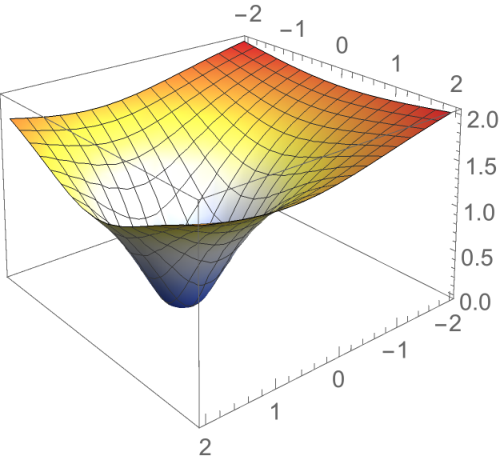
Figure 1: The setting in Ex. 1
(a) X1:n,T1:n{{X_{1:n}},{T_{1:n}}}
Refer to caption
(b) μ1​(x)\mu_{1}(x)
(c) π∗​(x)\pi^{*}(x)
Table 1: Policy evaluation performance in Ex. 1
Weights WW Vanilla τ^W\hat{\tau}_{W} Doubly robust τ^W,μ^\hat{\tau}_{W,\hat{\mu}} ‖W‖0\|W\|_{0}
RMSE Bias SD RMSE Bias SD
IPW, φ\varphi 2.2092.209 −0.005-0.005 2.2092.209 4.1964.196 0.4350.435 4.1744.174 13.6±2.913.6\pm 2.9
IPW, φ^\hat{\varphi} 0.5680.568 −0.514-0.514 0.2420.242 0.4280.428 0.2300.230 0.3610.361 13.6±2.913.6\pm 2.9
.05.05-CIPW, φ\varphi 0.5810.581 −0.491-0.491 0.3100.310 0.5200.520 0.2590.259 0.4510.451 13.6±2.913.6\pm 2.9
.05.05-CIPW, φ^\hat{\varphi} 0.5680.568 −0.514-0.514 0.2420.242 0.4280.428 0.2300.230 0.3610.361 13.6±2.913.6\pm 2.9
NIPW, φ\varphi 0.5190.519 −0.181-0.181 0.4870.487 0.7540.754 0.4080.408 0.6340.634 13.6±2.913.6\pm 2.9
NIPW, φ^\hat{\varphi} 0.4630.463 −0.251-0.251 0.3900.390 0.6920.692 0.4670.467 0.5110.511 13.6±2.913.6\pm 2.9
.05.05-NCIPW, φ\varphi 0.4850.485 −0.250-0.250 0.4150.415 0.7240.724 0.4710.471 0.5500.550 13.6±2.913.6\pm 2.9
.05.05-NCIPW, φ^\hat{\varphi} 0.4630.463 −0.251-0.251 0.3900.390 0.6920.692 0.4670.467 0.5110.511 13.6±2.913.6\pm 2.9
Balanced eval 0.280\mathbf{0.280} 0.2270.227 0.1630.163 0.251\mathbf{0.251} −0.006-0.006 0.2510.251 90.7±3.290.7\pm 3.2

Balanced policy evaluation seeks weights WW to minimize a combination of imbalance, given by the worst-case value of B⁡(W,π,f)B(W,\pi;f) over functions ff, and variance, given by the norm of weights WT​Λ​WW^{T}\Lambda W for a specified positive semidefinite (PSD) matrix Λ\Lambda. This follows a general approach introduced by [22, 24] of finding optimal balancing weights that optimize a given CMSE objective directly rather than via a plug-in approach. Any choice of ∥⋅∥\|\cdot\| gives rise to a worst-case CMSE objective for policy evaluation:

𝔈2(W,π;∥⋅∥,Λ)=sup‖f‖≤1B2(W,π;f)+1n2WTΛW.\textstyle\mathfrak{E}^{2}(W,\pi;\|\cdot\|,\Lambda)=\sup_{\|f\|\leq 1}B^{2}(W,\pi;f)+\frac{1}{n^{2}}W^{T}\Lambda W.

Here, we focus on ∥⋅∥\|\cdot\| given by the direct product of reproducing kernel Hilbert spaces (RKHS):

∥f∥p,𝒦1:m,γ1:m=(∑t=1m∥ft∥𝒦tp/γtp)1/p,\textstyle\|f\|_{p,\mathcal{K}_{1:m},\gamma_{1:m}}=(\sum_{t=1}^{m}\|f_{t}\|_{\mathcal{K}_{t}}^{p}/\gamma_{t}^{p})^{1/p},

where ∥⋅∥𝒦t\|\cdot\|_{\mathcal{K}_{t}} is the norm of the RKHS given by the PSD kernel 𝒦t​(⋅,⋅):𝒳2→ℝ\mathcal{K}_{t}(\cdot,\cdot):\mathcal{X}^{2}\to\mathbb{R}, i.e., the unique completion of span(𝒦t(x,⋅):x∈𝒳)\operatorname{span}(\mathcal{K}_{t}(x,\cdot):x\in\mathcal{X}) endowed with ⟨𝒦t​(x,⋅),𝒦t​(x′,⋅)⟩=𝒦t​(x,x′)\left<\mathcal{K}_{t}(x,\cdot),\mathcal{K}_{t}(x^{\prime},\cdot)\right>=\mathcal{K}_{t}(x,x^{\prime}) [39, see]. We say ‖f‖𝒦t=∞\|f\|_{\mathcal{K}_{t}}=\infty if ff is not in the RKHS. One example of a kernel is the Mahalanobis RBF kernel: 𝒦s(x,x′)=exp(−(x−x′)TS^−1(x−x′)/s2)\mathcal{K}_{s}(x,x^{\prime})=\exp(-(x-x^{\prime})^{T}\hat{S}^{-1}(x-x^{\prime})/s^{2}) where S^\hat{S} is the sample covariance of X1:nX_{1:n} and ss is a parameter. For such an RKHS product norm, we can decompose the worst-case objective into the discrepancies in each treatment as well as characterize it as a posterior (rather than worst-case) risk.

Lemma 1.

Let 𝔅t2(W,πt;∥⋅∥𝒦t)=∑i,j=1n(WiδTi​t−πt(Xi))(WjδTj​t−πt(Xj))𝒦t(Xi,Xj)\mathfrak{B}^{2}_{t}(W,\pi_{t};\|\cdot\|_{\mathcal{K}_{t}})=\sum_{i,j=1}^{n}(W_{i}\delta_{T_{i}t}-\pi_{t}(X_{i}))(W_{j}\delta_{T_{j}t}-\pi_{t}(X_{j}))\mathcal{K}_{t}(X_{i},X_{j}) and 1/p+1/q=11/p+1/q=1. Then

𝔈2(W,π;∥⋅∥p,𝒦1:m,γ1:m,Λ)=(∑t=1mγtq𝔅tq(W,πt;∥⋅∥𝒦t))2/q+1n2WTΛW.\textstyle\mathfrak{E}^{2}(W,\pi;\|\cdot\|_{p,\mathcal{K}_{1:m},\gamma_{1:m}},\Lambda)=(\sum_{t=1}^{m}\gamma_{t}^{q}\mathfrak{B}_{t}^{q}(W,\pi_{t};\|\cdot\|_{\mathcal{K}_{t}}))^{2/q}+\frac{1}{n^{2}}W^{T}\Lambda W.

Moreover, if p=2p=2 and μt\mu_{t} has a Gaussian process prior [44] with mean ftf_{t} and covariance γt​𝒦t\gamma_{t}\mathcal{K}_{t} then

CMSE(τ^W,f,π)=𝔈2(W,π;∥⋅∥p,𝒦1:m,γ1:m,Σ),\operatorname{CMSE}(\hat{\tau}_{W,f},\pi)=\mathfrak{E}^{2}(W,\pi;\|\cdot\|_{p,\mathcal{K}_{1:m},\gamma_{1:m}},\Sigma),

where the CMSE marginalizes over μ\mu. This gives the CMSE of τ^W\hat{\tau}_{W} for ff constant or τ^W,μ^\hat{\tau}_{W,\hat{\mu}} for f=μ^f=\hat{\mu}.

The second statement in Lemma 1 suggests that, in practice, model selection of γ1:m\gamma_{1:m}, Λ\Lambda, and kernel hyperparameters such as ss or even S^\hat{S}, can done by the marginal likelihood method [see 44, Ch. 5].

2.2 Evaluation Using Optimal Balancing Weights

Our policy evaluation estimates are given by either the estimator τ^W∗(π;∥⋅∥,Λ)\hat{\tau}_{W^{*}(\pi;\|\cdot\|,\Lambda)} or τ^W∗(π;∥⋅∥,Λ),μ^\hat{\tau}_{W^{*}(\pi;\|\cdot\|,\Lambda),\hat{\mu}} where W∗(π)=W∗(π;∥⋅∥,Λ)W^{*}(\pi)=W^{*}(\pi;\|\cdot\|,\Lambda) is the minimizer of 𝔈2(W,π;∥⋅∥,Λ)\mathfrak{E}^{2}(W,\pi;\|\cdot\|,\Lambda) over the space of all weights WW that sum to nn, 𝒲={W∈ℝ+n:∑i=1nWi=n}=n​Δn\mathcal{W}=\{W\in\mathbb{R}^{n}_{+}:\sum_{i=1}^{n}W_{i}=n\}=n\Delta^{n}. Specifically,

W∗(π;∥⋅∥,Λ)∈argminW∈𝒲𝔈2(W,π;∥⋅∥,Λ).\textstyle W^{*}(\pi;\|\cdot\|,\Lambda)\in\operatornamewithlimits{argmin}_{W\in\mathcal{W}}\mathfrak{E}^{2}(W,\pi;\|\cdot\|,\Lambda).

When ∥⋅∥=∥⋅∥p,𝒦1:m,γ1:m\|\cdot\|=\|\cdot\|_{p,\mathcal{K}_{1:m},\gamma_{1:m}}, this problem is a quadratic program for p=2p=2 and a second-order cone program for p=1,∞p=1,\infty. Both are efficiently solvable [9]. In practice, we solve these using Gurobi 7.0.

In Lemma 1, 𝔅t(W,πt;∥⋅∥𝒦t)\mathfrak{B}_{t}(W,\pi_{t};\|\cdot\|_{\mathcal{K}_{t}}) measures the imbalance between νt,π\nu_{t,\pi} and νt,W\nu_{t,W} as the worst-case discrepancy in means over functions in the unit ball of an RKHS. In fact, as a distributional distance metric, it is the maximum mean discrepancy (MMD) used, for example, for testing whether two samples come from the same distribution [16]. Thus, minimizing 𝔈2(W,π;∥⋅∥p,𝒦1:m,γ1:m,Λ)\mathfrak{E}^{2}(W,\pi;\|\cdot\|_{p,\mathcal{K}_{1:m},\gamma_{1:m}},\Lambda) is simply seeking the weights WW that balance νt,π\nu_{t,\pi} and νt,W\nu_{t,W} subject to variance regularization in WW.

Example 1.

We demonstrate balanced evaluation with a mixture of m=5m=5 Gaussians: X|T∼𝒩⁡(X¯T,I2×2)X\mid T\sim\mathcal{N}(\overline{X}_{T},I_{2\times 2}), X¯1=(0,0)\overline{X}_{1}=(0,0), X¯t=(Re,Im)​(ei​2​π​(t−2)/(m−1))\overline{X}_{t}=(\operatorname{Re},\operatorname{Im})(e^{i2\pi(t-2)/(m-1)}) for t=2,…,mt=2,\dots,m, and T∼Multinomial⁡(1/5,…,1/5)T\sim\operatorname{Multinomial}(1/5,\dots,1/5). Fix a draw of X1:n,T1:n{{X_{1:n}},{T_{1:n}}} with n=100n=100 shown in Fig. 1(a) (numpy seed 0). Color denotes TiT_{i} and size denotes φTi​(Xi)\varphi_{T_{i}}(X_{i}). The centers X¯t\overline{X}_{t} are marked by a colored number. Next, we let μt​(x)=exp⁡(1−1/‖x−χt‖2)\mu_{t}(x)=\exp(1-1/\|x-\chi_{t}\|_{2}) where χt=(Re,Im)(e−i2πt/m/2)\chi_{t}=(\operatorname{Re},\operatorname{Im})(e^{-i2\pi t/m}/\sqrt{2}) for t∈[m]t\in[m], ϵi∼𝒩⁡(0,σ)\epsilon_{i}\sim\mathcal{N}(0,\sigma), and σ=1\sigma=1. Fig. 1(b) plots μ1​(x)\mu_{1}(x). Fig. 1(c) shows the corresponding optimal policy π∗\pi^{*}.

Next we consider evaluating π∗\pi^{*}. Fixing X1:n{X_{1:n}} as in Fig. 1(a), we have SAPE⁡(π∗)=0.852\operatorname{SAPE}(\pi^{*})=0.852. With X1:n{X_{1:n}} fixed, we draw 1000 replications of T1:n,Y1:n{T_{1:n}},{Y_{1:n}} from their conditional distribution. For each replication, we fit φ^\hat{\varphi} by estimating the (well-specified) Gaussian mixture by maximum likelihood and fit μ^\hat{\mu} using mm separate gradient-boosted tree models (sklearn defaults). We consider evaluating π∗\pi^{*} either using the vanilla estimator τ^W\hat{\tau}_{W} or the doubly robust estimator τ^W,μ^\hat{\tau}_{W,\hat{\mu}} for WW either chosen in the 4 different standard ways laid out in Sec. 1.2, using either the true φ\varphi or the estimated φ^\hat{\varphi}, or chosen by the balanced evaluation approach using untuned parameters (rather than fit by marginal likelihood) using the standard (s=1s=1) Mahalanobis RBF kernel for 𝒦t\mathcal{K}_{t}, ‖f‖2=∑t=1m‖ft‖𝒦t2\|f\|^{2}=\sum_{t=1}^{m}\|f_{t}\|_{\mathcal{K}_{t}}^{2}, and Λ=I\Lambda=I. (Note that this misspecifies the outcome model, ‖μt‖𝒦t=∞\|\mu_{t}\|_{\mathcal{K}_{t}}=\infty.) We tabulate the results in Tab. 1.

We note a few observations on the standard approaches: vanilla IPW with true φ\varphi has zero bias but large SD (standard deviation) and hence RMSE (root mean square error); a DR approach improves on a vanilla IPW with φ^\hat{\varphi} by reducing bias; clipping and normalizing IPW reduces SD. The balanced evaluation approach achieves the best RMSE by a clear margin, with the vanilla estimator beating all standard vanilla and DR estimators and the DR estimator providing a further improvement by nearly eliminating bias (but increasing SD). The marked success of the balanced approach is unsurprising when considering the support ∥W∥0=∑i=1n𝕀[Wi>0]\|W\|_{0}=\sum_{i=1}^{n}\mathbb{I}\left[W_{i}>0\right] of the weights. All standard approaches use weights that are multiples of πTi​(Xi)\pi_{T_{i}}(X_{i}), limiting support to the overlap between π\pi and T1:n{T_{1:n}}, which hovers around 1010–1616 over replications. The balanced approach uses weights that have significantly wider support, around 8888–9494. In light of this, the success of the balanced approach is expected.

2.3 Consistent Evaluation

Next we consider the question of consistent evaluation: under what conditions can we guarantee that τ^W∗​(π)−SAPE⁡(π)\hat{\tau}_{W^{*}(\pi)}-\operatorname{SAPE}(\pi) and τ^W∗​(π),μ^−SAPE⁡(π)\hat{\tau}_{W^{*}(\pi),\hat{\mu}}-\operatorname{SAPE}(\pi) converge to zero and at what rates.

One key requirement for consistent evaluation is a weak form of overlap between the historical data and the target policy to be evaluated using this data:

Assumption 2 (Weak overlap).

ℙ⁡(φt​(X)>0∨πt​(X)=0)=1​∀t∈[m]\mathbb{P}(\varphi_{t}(X)>0\vee\pi_{t}(X)=0)=1\,\forall t\in[m], 𝔼⁡[πT2​(X)/φT2​(X)]<∞\mathbb{E}[{{{\pi^{2}_{T}(X)}/{\varphi^{2}_{T}(X)}}}]<\infty.

This ensures that if π\pi can assign treatment tt to XX then the data will have some examples of units with similar covariates being given treatment tt; otherwise, we can never say what the outcome might look like. Another key requirement is specification. If the mean-outcome function is well-specified in that it is in the RKHS product used to compute W∗​(π)W^{*}(\pi) then convergence at rate 1/n1/\sqrt{n} is guaranteed. Otherwise, for a doubly robust estimator, if the regression estimate is well-specified then consistency is still guaranteed. In lieu of specification, consistency is also guaranteed if the RKHS product consists of C0C_{0}-universal kernels, defined below, such as the RBF kernel [40].

Definition 1.

A PSD kernel 𝒦\mathcal{K} on a Hausdorff 𝒳\mathcal{X} (e.g., ℝd\mathbb{R}^{d}) is C0C_{0}-universal if, for any continuous function g:𝒳→ℝg:\mathcal{X}\to\mathbb{R} with compact support (i.e., for some CC compact, {x:g⁡(x)≠0}⊆C\{x:g(x)\neq 0\}\subseteq C) and η>0\eta>0, there exists m,α1,x1,…,αm,xmm,\alpha_{1},x_{1},\dots,\alpha_{m},x_{m} such that supx∈𝒳|∑j=1mαi​𝒦​(xj,x)−g⁡(x)|≤η\sup_{x\in\mathcal{X}}|\sum_{j=1}^{m}\alpha_{i}\mathcal{K}(x_{j},x)-g(x)|\leq\eta.

Figure 2: Policy learning results in Ex. 2; numbers denote regret

.        Balanced policy learner .06

    IPW .50     Gauss Proc 0.29     IPW-SVM 0.34     SNPOEM 0.28
    DR .26     Grad Boost 0.20     DR-SVM 0.18     PF 0.23
Theorem 3.

Fix π\pi and let Wn∗(π)=Wn∗(π;∥f∥p,𝒦1:m,γn,1:m,Λn)W_{n}^{*}(\pi)=W_{n}^{*}(\pi;\|f\|_{p,\mathcal{K}_{1:m},\gamma_{n,1:m}},\Lambda_{n}) with 0≺κ¯​I⪯Λn⪯κ¯​I0\prec\underline{\kappa}I\preceq\Lambda_{n}\preceq\overline{\kappa}I, 0<γ¯≤γn,t≤γ¯​∀t∈[m]0<\underline{\gamma}\leq\gamma_{n,t}\leq\overline{\gamma}\,\forall t\in[m] for each nn. Suppose Asns. 1 and 2 hold, Var⁡(Y∣X)\operatorname{Var}(Y\mid X) a.s. bounded, 𝔼⁡[𝒦t​(X,X)]<∞\mathbb{E}[{\sqrt{\mathcal{K}_{t}(X,X)}}]<\infty, and 𝔼⁡[𝒦t​(X,X)​πT2​(X)/φT2​(X)]<∞\mathbb{E}[{\mathcal{K}_{t}(X,X){{\pi^{2}_{T}(X)}/{\varphi^{2}_{T}(X)}}}]<\infty. Then the following two results hold:

  1. (a)

    If ‖μt‖𝒦t<∞\|\mu_{t}\|_{\mathcal{K}_{t}}<\infty for all t∈[m]t\in[m]: τ^Wn∗​(π)−SAPE⁡(π)=Op​(1/n).{\hat{\tau}_{W_{n}^{*}(\pi)}-\operatorname{SAPE}(\pi)}=O_{p}(1/\sqrt{n}).

  2. (b)

    If 𝒦t\mathcal{K}_{t} is C0C_{0}-universal for all t∈[m]t\in[m]: τ^Wn∗​(π)−SAPE⁡(π)=op​(1){\hat{\tau}_{W_{n}^{*}(\pi)}-\operatorname{SAPE}(\pi)}=o_{p}(1).

The key assumptions of Thm. 3 are unconfoundedness, overlap, and bounded variance. The other conditions simply guide the choice of method parameters. The two conditions on the kernel are trivial for bounded kernels like the RBF kernel. An analogous result for the DR estimator is a corollary.

Corollary 4.

Suppose the assumptions of Thm. 3 hold and. Then

  1. (a)

    If ‖μ^n​t−μt‖𝒦t=op​(1)​∀t∈[m]\|\hat{\mu}_{nt}-\mu_{t}\|_{\mathcal{K}_{t}}=o_{p}(1)\,\forall t\in[m]:
    . τ^Wn∗​(π),μ^n−SAPE⁡(π)=(1n2​∑i=1nWn​i∗2​Var⁡(Yi∣Xi))1/2+op​(1/n).{\hat{\tau}_{W_{n}^{*}(\pi),\hat{\mu}_{n}}-\operatorname{SAPE}(\pi)}=(\frac{1}{n^{2}}\sum_{i=1}^{n}{W^{*}_{ni}}^{2}\operatorname{Var}(Y_{i}\mid X_{i}))^{1/2}+o_{p}(1/\sqrt{n}).

  2. (b)

    If ‖μ^n​(X)−μ⁡(X)‖2=Op​(r⁡(n))\|\hat{\mu}_{n}(X)-\mu(X)\|_{2}=O_{p}(r(n)), r⁡(n)=Ω⁡(1/n)r(n)=\Omega(1/\sqrt{n}): τ^Wn∗​(π),μ^n−SAPE⁡(π)=Op​(r⁡(n)).{\hat{\tau}_{W_{n}^{*}(\pi),\hat{\mu}_{n}}-\operatorname{SAPE}(\pi)}=O_{p}(r(n)).

  3. (c)

    If ‖μt‖𝒦t<∞,‖μ^n​t‖𝒦t=Op​(1)\|\mu_{t}\|_{\mathcal{K}_{t}}<\infty,\|\hat{\mu}_{nt}\|_{\mathcal{K}_{t}}=O_{p}(1) for all t∈[m]t\in[m]: τ^Wn∗​(π),μ^n−SAPE⁡(π)=Op​(1/n).{\hat{\tau}_{W_{n}^{*}(\pi),\hat{\mu}_{n}}-\operatorname{SAPE}(\pi)}=O_{p}(1/\sqrt{n}).

  4. (d)

    If 𝒦t\mathcal{K}_{t} is C0C_{0}-universal for all t∈[m]t\in[m]: τ^Wn∗​(π),μ^n−SAPE⁡(π)=op​(1){\hat{\tau}_{W_{n}^{*}(\pi),\hat{\mu}_{n}}-\operatorname{SAPE}(\pi)}=o_{p}(1).

Cor. 4(a) is the case where both the balancing weights and the regression function are well-specified, in which case the multiplicative bias disappears faster than op​(1/n)o_{p}(1/\sqrt{n}), leaving us only with the irreducible residual variance, leading to an efficient evaluation. The other cases concern the “doubly robust” nature of the balanced DR estimator: Cor. 4(b) requires only that the regression be consitent and Cor. 4(c)-(d) require only the balancing weights to be consistent.

3 Balanced Learning

Next we consider a balanced approach to policy learning. Given a policy class Π⊂[𝒳→Δm]\Pi\subset[\mathcal{X}\to\Delta^{m}], we let the balanced policy learner yield the policy π∈Π\pi\in\Pi that minimizes the balanced policy evaluation using either a vanilla or DR estimator plus a potential regularization term in the worst-case/posterior CMSE of the evaluation. We formulate this as a bilevel optimization problem:

π^bal\textstyle\textstyle\hat{\pi}^{\text{bal}} ∈argminπ{τ^W+λ𝔈(W,π;∥⋅∥,Λ):π∈Π,W∈argminW∈𝒲𝔈2(W,π;∥⋅∥,Λ)}\textstyle\in\operatornamewithlimits{argmin}_{\pi}\{\hat{\tau}_{W}\hskip 3.84995pt+\hskip-1.99997pt\lambda\mathfrak{E}(W,\pi;\|\cdot\|,\Lambda)\hskip-0.50003pt:\hskip-0.50003pt\pi\in\Pi,W\in\operatornamewithlimits{argmin}_{W\in\mathcal{W}}\mathfrak{E}^{2}(W,\pi;\|\cdot\|,\Lambda)\} (1)
π^bal-DR\textstyle\textstyle\hat{\pi}^{\text{bal-DR}} ∈argminπ{τ^W,μ^+λ𝔈(W,π;∥⋅∥,Λ):π∈Π,W∈argminW∈𝒲𝔈2(W,π;∥⋅∥,Λ)}\textstyle\in\operatornamewithlimits{argmin}_{\pi}\{\hat{\tau}_{W,\hat{\mu}}\hskip-1.99997pt+\hskip-1.99997pt\lambda\mathfrak{E}(W,\pi;\|\cdot\|,\Lambda)\hskip-0.50003pt:\hskip-0.50003pt\pi\in\Pi,W\in\operatornamewithlimits{argmin}_{W\in\mathcal{W}}\mathfrak{E}^{2}(W,\pi;\|\cdot\|,\Lambda)\} (2)

The regularization term regularizes both the balance (i.e., worst-case/posterior bias) that is achievable for π\pi and the variance in evaluating π\pi. We include this regularizer for completeness and motivated by the results of [42] (which regularize variance), but find that it not necessary to include it in practice.

3.1 Optimizing the Balanced Policy Learner

Unlike [7, 13, 1, 41, 45], our (nonconvex) policy optimization problem does not reduce to weighted classification precisely because our weights are not multiplies of πTi​(Xi)\pi_{T_{i}}(X_{i}) (but therefore our weights also lead to better performance). Instead, like [42], we use gradient descent. For that, we need to be able to differentiate our bilevel optimization problem. We focus on p=2p=2 for brevity.

Theorem 5.

Let ∥⋅∥=∥⋅∥2,𝒦1:m,γ1:m\|\cdot\|=\|\cdot\|_{2,\mathcal{K}_{1:m},\gamma_{1:m}}. Then ∃W∗(π)∈argminW∈𝒲𝔈2(W,π;∥⋅∥,Λ)\exists W^{*}(\pi)\in\operatornamewithlimits{argmin}_{W\in\mathcal{W}}\mathfrak{E}^{2}(W,\pi;\|\cdot\|,\Lambda) such that

∇πt​(X1),…,πt​(Xn)τ^W∗​(π)=1nY1:nTH~(I−(A+(I−A)H~)−1(I−A)H~)Jt\textstyle\nabla_{\pi_{t}(X_{1}),\dots,\pi_{t}(X_{n})}\hat{\tau}_{W^{*}(\pi)}=\frac{1}{n}Y_{1:n}^{T}\tilde{H}(I-(A+(I-A)\tilde{H})^{-1}(I-A)\tilde{H})J_{t}
∇πt​(X1),…,πt​(Xn)τ^W∗​(π),μ^=1nϵ^1:nTH~(I−(A+(I−A)H~)−1(I−A)H~)Jt+1nμ^t(X1:n)\textstyle\nabla_{\pi_{t}(X_{1}),\dots,\pi_{t}(X_{n})}\hat{\tau}_{W^{*}(\pi),\hat{\mu}}=\frac{1}{n}\hat{\epsilon}_{1:n}^{T}\tilde{H}(I-(A+(I-A)\tilde{H})^{-1}(I-A)\tilde{H})J_{t}+\frac{1}{n}\hat{\mu}_{t}({X_{1:n}})
∇πt​(X1),…,πt​(Xn)𝔈(W∗(π),π;∥⋅∥,Λ)=−Dt/𝔈(W∗(π),π;∥⋅∥,Λ)\textstyle\nabla_{\pi_{t}(X_{1}),\dots,\pi_{t}(X_{n})}\mathfrak{E}(W^{*}(\pi),\pi;\|\cdot\|,\Lambda)=-D_{t}/\mathfrak{E}(W^{*}(\pi),\pi;\|\cdot\|,\Lambda)

where H~=−F​(FT​H​F)−1​FT\tilde{H}=-F(F^{T}HF)^{-1}F^{T}, Fi​j=δi​j−δi​nF_{ij}=\delta_{ij}-\delta_{in} for i∈[n],j∈[n−1]i\in[n],j\in[n-1], Ai​j=δi​j𝕀[Wi∗(π)>0]A_{ij}=\delta_{ij}\mathbb{I}\left[W_{i}^{*}(\pi)>0\right], Dt​i=γt2​∑j=1n𝒦t​(Xi,Xj)​(Wj​δTj​t−πt​(Xj))D_{ti}=\gamma_{t}^{2}\sum_{j=1}^{n}\mathcal{K}_{t}(X_{i},X_{j})(W_{j}\delta_{T_{j}t}-\pi_{t}(X_{j})), Hi​j=2​∑t=1mγt2​δTi​t​δTj​t​𝒦t​(Xi,Xj)+2​ΛH_{ij}=2\sum_{t=1}^{m}\gamma_{t}^{2}\delta_{T_{i}t}\delta_{T_{j}t}\mathcal{K}_{t}(X_{i},X_{j})+2\Lambda, and Jt​i​j=−2​γt2​δTi​t​𝒦t​(Xi,Xj)J_{tij}=-2\gamma_{t}^{2}\delta_{T_{i}t}\mathcal{K}_{t}(X_{i},X_{j}).

To leverage this result, we use a parameterized policy class such as Πlogit={πt(x;βt)∝exp(βt​0+βtTx)}\Pi_{\text{logit}}=\{\pi_{t}(x;\beta_{t})\propto\exp(\beta_{t0}+\beta_{t}^{T}x)\} (or kernelized versions thereof), apply chain rule to differentiate objective in the parameters β\beta, and use BFGS [15] with random starts. The logistic parametrization allows us to smooth the problem even while the solution ends up being deterministic (extreme β\beta).

This approach requires solving a quadratic program for each objective gradient evaluation. While this can be made faster by using the previous solution as warm start, it is still computationally intensive, especially as the bilevel problem is nonconvex and both it and each quadratic program solved in “batch” mode. This is a limitation of the current optimization algorithm that we hope to improve on in the future using specialized methods for bilevel optimization [32, 4, 37].

Example 2.

We return to Ex. 1 and consider policy learning. We use the fixed draw shown in Fig. 1(a) and set σ\sigma to 0. We consider a variety of policy learners and plot the policies in Fig. 2 along with their population regret PAPE⁡(π)−PAPE⁡(π∗)\operatorname{PAPE}(\pi)-\operatorname{PAPE}(\pi^{*}). The policy learners we consider are: minimizing standard IPW and DR evaluations over Πlogit\Pi_{\text{logit}} with φ^,μ^\hat{\varphi},\hat{\mu} as in Ex. 1 (versions with combinations of normalized, clipped, and/or true φ\varphi, not shown, all have regret 0.26–0.5), the direct method with Gaussian process regression gradient boosted trees (both sklearn defaults), weighted SVM classification using IPW and DR weights (details in supplement), SNPOEM [43], PF [23], and our balanced policy learner (1) with parameters as in Ex. 1, Π=Πlogit,λ=Λ=0\Pi=\Pi_{\text{logit}},\lambda=\Lambda=0 (the DR version (2), not shown, has regret .08).

Example 3.

Next, we consider two UCI multi-class classification datasets [30], Glass (n=214n=214, d=9d=9, m=6m=6) and Ecoli (n=336n=336, d=7d=7, m=8m=8), and use a supervised-to-contextual-bandit transformation [7, 42, 13] to compare different policy learning algorithms. Given a supervised multi-class dataset, we draw TT as per a multilogit model with random ±1\pm 1 coefficients in the normalized covariates XX. Further, we set YY to 0 if TT matches the label and 1 otherwise. And we split the data 75-25 into training and test sample. Using 100 replications of this process, we evaluate the performance of learned linear policies by comparing the linear policy learners as in Ex. 2. For IPW-based approaches, we estimate φ^\hat{\varphi} by a multilogit regression (well-specified by construction). For DR approaches, we estimate μ^\hat{\mu} using gradient boosting trees (sklearn defaults). We compare these to our balanced policy learner in both vanilla and DR forms with all parameters fit by marginal likelihood using the RBF kernel with an unspecified length scale after normalizing the data. We tabulate the results in Tab. 2. They first demonstrate that employing the various stopgap fixes to IPW-based policy learning as in SNPOEM indeed provides a critical edge. This is further improved upon by using a balanced approach to policy learning, which gives the best results. In this example, DR approaches do worse than vanilla ones, suggesting both that XGBoost provided a bad outcome model and/or that the additional variance of DR was not compensated for by sufficiently less bias.

Table 2: Policy learning results in Ex. 3
IPW DR IPW-SVM DR-SVM POEM SNPOEM Balanced Balanced-DR
Glass 0.726 0.755 0.641 0.731 0.851 0.615 0.584 0.660
Ecoli 0.488 0.501 0.332 0.509 0.431 0.331 0.298 0.371

3.2 Uniform Consistency and Regret Bounds

Next, we establish consistency results uniformly over policy classes. This allows us to bound the regret of the balanced policy learner. We define the sample and population regret, respectively, as

RΠ​(π^)=PAPE⁡(π^)−minπ∈Π⁡PAPE⁡(π),R^Π​(π^)=SAPE⁡(π^)−minπ∈Π⁡SAPE⁡(π)\textstyle R_{\Pi}(\hat{\pi})=\operatorname{PAPE}(\hat{\pi})-\min_{\pi\in\Pi}\operatorname{PAPE}(\pi),\quad\widehat{R}_{\Pi}(\hat{\pi})=\operatorname{SAPE}(\hat{\pi})-\min_{\pi\in\Pi}\operatorname{SAPE}(\pi)

A key requirement for these to converge is that the best-in-class policy is learnable. We quantify that using Rademacher complexity [3] and later extend our results to VC dimension. Let us define

ℜ^n​(ℱ)=12n​∑ρi∈{−1,+1}nsupf∈ℱ1n​∑i=1nρi​f​(Xi),ℜn​(ℱ)=𝔼⁡[ℜ^n​(ℱ)].\textstyle\widehat{\mathfrak{R}}_{n}(\mathcal{F})=\frac{1}{2^{n}}\sum_{\rho_{i}\in\{-1,+1\}^{n}}\sup_{f\in\mathcal{F}}\frac{1}{n}\sum_{i=1}^{n}\rho_{i}f(X_{i}),\quad{\mathfrak{R}}_{n}(\mathcal{F})=\mathbb{E}[{\widehat{\mathfrak{R}}_{n}(\mathcal{F})}].

E.g., for linear policies ℜ^n​(ℱ)=O⁡(1/n)\widehat{\mathfrak{R}}_{n}(\mathcal{F})=O(1/\sqrt{n}) [21]. If ℱ⊆[𝒳→ℝm]\mathcal{F}\subseteq[\mathcal{X}\to\mathbb{R}^{m}] let ℱt={(f⁡(⋅))t:f∈ℱ}\mathcal{F}_{t}=\{(f(\cdot))_{t}:f\in\mathcal{F}\} and set ℜn​(ℱ)=∑t=1mℜn​(ℱt){\mathfrak{R}}_{n}(\mathcal{F})=\sum_{t=1}^{m}{\mathfrak{R}}_{n}(\mathcal{F}_{t}) and same for ℜ^n​(ℱ)\widehat{\mathfrak{R}}_{n}(\mathcal{F}). We also strengthen the overlap assumption.

Assumption 3 (Strong overlap).

∃α≥1\exists\alpha\geq 1 such that ℙ⁡(φt​(X)≥1/α)=1\mathbb{P}(\varphi_{t}(X)\geq 1/\alpha)=1 ∀t∈[m]\forall t\in[m].

Theorem 6.

Fix Π⊆[𝒳→Δm]\Pi\subseteq[\mathcal{X}\to\Delta^{m}] and let Wn∗(π)=Wn∗(π;∥f∥p,𝒦1:m,γn,1:m,Λn)W_{n}^{*}(\pi)=W_{n}^{*}(\pi;\|f\|_{p,\mathcal{K}_{1:m},\gamma_{n,1:m}},\Lambda_{n}) with 0≺κ¯​I⪯Λn⪯κ¯​I0\prec\underline{\kappa}I\preceq\Lambda_{n}\preceq\overline{\kappa}I, 0<γ¯≤γn,t≤γ¯​∀t∈[m]0<\underline{\gamma}\leq\gamma_{n,t}\leq\overline{\gamma}\,\forall t\in[m] for each nn and π∈Π\pi\in\Pi. Suppose Asns. 1 and 3 hold, |ϵi|≤B\left|\epsilon_{i}\right|\leq B a.s. bounded, and 𝒦t​(x,x)≤Γ​∀t∈[m]\sqrt{\mathcal{K}_{t}(x,x)}\leq\Gamma\,\forall t\in[m] for Γ≥1\Gamma\geq 1. Then the following two results hold:

  1. (a)

    If ‖μt‖𝒦t<∞,∀t∈[m]\|\mu_{t}\|_{\mathcal{K}_{t}}<\infty,\,\forall t\in[m] then for nn sufficiently large (n≥2​log⁡(4​m/ν)/(1/(2​α)−ℜn​(Π))2n\geq 2\log(4m/\nu)/(1/(2\alpha)-{\mathfrak{R}}_{n}(\Pi))^{2}), we have that, with probability at least 1−ν1-\nu,

    supπ∈Π|τ^W∗​(π)−SAPE⁡(π)|≤\textstyle\hskip-21.00009pt\sup_{\pi\in\Pi}|\hat{\tau}_{W^{*}(\pi)}-\operatorname{SAPE}(\pi)|\leq 8​α​Γ​γ¯​m​(‖μ‖+2​log⁡(4​m/ν)​κ¯−1​B)​ℜn​(Π)\textstyle 8\alpha\Gamma\overline{\gamma}m(\|\mu\|+\sqrt{2\log(4m/\nu)}\underline{\kappa}^{-1}B){\mathfrak{R}}_{n}(\Pi)
    +1n​(2​α​κ¯​‖μ‖+12​α​Γ2​γ¯​m​‖μ‖+6​α​Γ​γ¯​m​κ¯−1​B​log⁡(4​mν))\textstyle+\frac{1}{\sqrt{n}}\left({2\alpha\overline{\kappa}\|\mu\|+12\alpha\Gamma^{2}\overline{\gamma}m\|\mu\|}+6\alpha\Gamma\overline{\gamma}m\underline{\kappa}^{-1}B\log\left(\frac{4m}{\nu}\right)\right)
    +1n​(2​α​κ¯​κ¯−1​B+12​α​Γ2​γ¯​m​κ¯−1​B+3​α​Γ​γ¯​m​‖μ‖)​2​log⁡(4​mν)\textstyle+\frac{1}{\sqrt{n}}(2\alpha\overline{\kappa}\underline{\kappa}^{-1}B+12\alpha\Gamma^{2}\overline{\gamma}m\underline{\kappa}^{-1}B+3\alpha\Gamma\overline{\gamma}m\|\mu\|)\sqrt{2\log\left(\frac{4m}{\nu}\right)}
  2. (b)

    If 𝒦t\mathcal{K}_{t} is C0C_{0}-universal for all t∈[m]t\in[m] and either ℜn​(Π)=o​(1)\textstyle{\mathfrak{R}}_{n}(\Pi)=o(1) or ℜ^n​(Π)=op​(1)\textstyle\widehat{\mathfrak{R}}_{n}(\Pi)=o_{p}(1) then

    supπ∈Π|τ^W∗​(π)−SAPE⁡(π)|=op​(1).\textstyle\sup_{\pi\in\Pi}|\hat{\tau}_{W^{*}(\pi)}-\operatorname{SAPE}(\pi)|=o_{p}(1).

The proof crucially depends on simultaneously handling the functional complexities of both the policy class Π\Pi and the space of functions {f:‖f‖<∞}\{f:\|f\|<\infty\} being balanced against. Again, the key assumptions of Thm. 6 are unconfoundedness, overlap, and bounded residuals. The other conditions simply guide the choice of method parameters. Regret bounds follow as a corollary.

Corollary 7.

Suppose the assumptions of Thm. 6 hold. If π^nbal\hat{\pi}_{n}^{\text{bal}} is as in (1) then:

  1. (a)

    If ‖μt‖𝒦t<∞\|\mu_{t}\|_{\mathcal{K}_{t}}<\infty for all t∈[m]t\in[m]: RΠ​(π^nbal)=Op​(ℜn​(Π)+1/n).\textstyle R_{\Pi}(\hat{\pi}_{n}^{\text{bal}})=O_{p}(\mathfrak{R}_{n}(\Pi)+1/\sqrt{n}).

  2. (b)

    If 𝒦t\mathcal{K}_{t} is C0C_{0}-universal for all t∈[m]t\in[m]: RΠ​(π^nbal)=op​(1).\textstyle R_{\Pi}(\hat{\pi}_{n}^{\text{bal}})=o_{p}(1).

If π^nbal-DR\hat{\pi}_{n}^{\text{bal-DR}} is as in (2) then:

  1. (c)

    If ‖μ^n​t−μt‖𝒦t=op​(1)\|\hat{\mu}_{nt}-\mu_{t}\|_{\mathcal{K}_{t}}=o_{p}(1) for all t∈[m]t\in[m]: RΠ​(π^nbal-DR)=Op​(ℜn​(Π)+1/n).\textstyle R_{\Pi}(\hat{\pi}_{n}^{\text{bal-DR}})=O_{p}(\mathfrak{R}_{n}(\Pi)+1/\sqrt{n}).

  2. (d)

    If ‖μ^n​(X)−μ⁡(X)‖2=Op​(r⁡(n))\|\hat{\mu}_{n}(X)-\mu(X)\|_{2}=O_{p}(r(n)): RΠ​(π^nbal-DR)=Op​(r⁡(n)+ℜn​(Π)+1/n).\textstyle R_{\Pi}(\hat{\pi}_{n}^{\text{bal-DR}})=O_{p}(r(n)+\mathfrak{R}_{n}(\Pi)+1/\sqrt{n}).

  3. (e)

    If ‖μt‖𝒦t<∞,‖μ^n​t‖𝒦t=Op​(1)\|\mu_{t}\|_{\mathcal{K}_{t}}<\infty,\|\hat{\mu}_{nt}\|_{\mathcal{K}_{t}}=O_{p}(1) for all t∈[m]t\in[m]: RΠ​(π^nbal-DR)=Op​(ℜn​(Π)+1/n).\textstyle R_{\Pi}(\hat{\pi}_{n}^{\text{bal-DR}})=O_{p}(\mathfrak{R}_{n}(\Pi)+1/\sqrt{n}).

  4. (f)

    If 𝒦t\mathcal{K}_{t} is C0C_{0}-universal for all t∈[m]t\in[m]: RΠ​(π^nbal)=op​(1).\textstyle R_{\Pi}(\hat{\pi}_{n}^{\text{bal}})=o_{p}(1).

And, all the same results hold when replacing ℜn​(Π){\mathfrak{R}}_{n}(\Pi) with ℜ^n​(Π)\widehat{\mathfrak{R}}_{n}(\Pi) and/or replacing RΠR_{\Pi} with R^Π\widehat{R}_{\Pi}.

4 Conclusion

Considering the policy evaluation and learning problems using observational or logged data, we presented a new method that is based on finding optimal balancing weights that make the data look like the target policy and that is aimed at ameliorating the shortcomings of existing methods, which included having to deal with near-zero propensities, using too few positive weights, and using an awkward two-stage procedure. The new approach showed promising signs of fixing these issues in some numerical examples. However, the new learning method is more computationally intensive than existing approaches, solving a QP at each gradient step. Therefore, in future work, we plan to explore faster algorithms that can implement the balanced policy learner, perhaps using alternating descent, and use these to investigate comparative numerics in much larger datasets.

Acknowledgements

This material is based upon work supported by the National Science Foundation under Grant No. 1656996.

References

  • [1] S. Athey and S. Wager. Efficient policy learning. arXiv preprint arXiv:1702.02896, 2017.
  • [2] P. C. Austin and E. A. Stuart. Moving towards best practice when using inverse probability of treatment weighting (iptw) using the propensity score to estimate causal treatment effects in observational studies. Statistics in medicine, 34(28):3661–3679, 2015.
  • [3] P. L. Bartlett and S. Mendelson. Rademacher and gaussian complexities: Risk bounds and structural results. The Journal of Machine Learning Research, 3:463–482, 2003.
  • [4] K. P. Bennett, G. Kunapuli, J. Hu, and J.-S. Pang. Bilevel optimization and machine learning. In IEEE World Congress on Computational Intelligence, pages 25–47. Springer, 2008.
  • [5] D. Bertsimas and N. Kallus. The power and limits of predictive approaches to observational-data-driven optimization. arXiv preprint arXiv:1605.02347, 2016.
  • [6] D. Bertsimas, N. Kallus, A. M. Weinstein, and Y. D. Zhuo. Personalized diabetes management using electronic medical records. Diabetes care, 40(2):210–217, 2017.
  • [7] A. Beygelzimer and J. Langford. The offset tree for learning with partial labels. In Proceedings of the 15th ACM SIGKDD international conference on Knowledge discovery and data mining, pages 129–138. ACM, 2009.
  • [8] L. Bottou, J. Peters, J. Q. Candela, D. X. Charles, M. Chickering, E. Portugaly, D. Ray, P. Y. Simard, and E. Snelson. Counterfactual reasoning and learning systems: the example of computational advertising. Journal of Machine Learning Research, 14(1):3207–3260, 2013.
  • [9] S. P. Boyd and L. Vandenberghe. Convex Optimization. Cambridge University Press, Cambridge, 2004.
  • [10] S. Bubeck and N. Cesa-Bianchi. Regret analysis of stochastic and nonstochastic multi-armed bandit problems. Foundations and Trends in Machine Learning, 5(1):1–122, 2012.
  • [11] V. Chernozhukov, D. Chetverikov, M. Demirer, E. Duflo, and C. Hansen. Double machine learning for treatment and causal parameters. arXiv preprint arXiv:1608.00060, 2016.
  • [12] K. Crammer and Y. Singer. On the algorithmic implementation of multiclass kernel-based vector machines. Journal of machine learning research, 2(Dec):265–292, 2001.
  • [13] M. Dudík, J. Langford, and L. Li. Doubly robust policy evaluation and learning. arXiv preprint arXiv:1103.4601, 2011.
  • [14] M. R. Elliott. Model averaging methods for weight trimming. Journal of official statistics, 24(4):517, 2008.
  • [15] R. Fletcher. Practical methods of optimization. John Wiley & Sons, 2013.
  • [16] A. Gretton, K. M. Borgwardt, M. Rasch, B. Schölkopf, and A. J. Smola. A kernel method for the two-sample-problem. In Advances in neural information processing systems, pages 513–520, 2006.
  • [17] D. G. Horvitz and D. J. Thompson. A generalization of sampling without replacement from a finite universe. Journal of the American statistical Association, 47(260):663–685, 1952.
  • [18] G. W. Imbens. The role of the propensity score in estimating dose-response functions. Biometrika, 87(3), 2000.
  • [19] G. W. Imbens and D. B. Rubin. Causal inference in statistics, social, and biomedical sciences. Cambridge University Press, 2015.
  • [20] E. L. Ionides. Truncated importance sampling. Journal of Computational and Graphical Statistics, 17(2):295–311, 2008.
  • [21] S. M. Kakade, K. Sridharan, and A. Tewari. On the complexity of linear prediction: Risk bounds, margin bounds, and regularization. In Advances in neural information processing systems, pages 793–800, 2009.
  • [22] N. Kallus. Generalized optimal matching methods for causal inference. arXiv preprint arXiv:1612.08321, 2016.
  • [23] N. Kallus. Recursive partitioning for personalization using observational data. In International Conference on Machine Learning (ICML), pages 1789–1798, 2017.
  • [24] N. Kallus. Optimal a priori balance in the design of controlled experiments. Journal of the Royal Statistical Society: Series B (Statistical Methodology), 80(1):85–112, 2018.
  • [25] N. Kallus and A. Zhou. Confounding-robust policy improvement. 2018a.
  • [26] N. Kallus and A. Zhou. Policy evaluation and optimization with continuous treatments. In International Conference on Artificial Intelligence and Statistics, pages 1243–1251, 2018b.
  • [27] J. D. Kang, J. L. Schafer, et al. Demystifying double robustness: A comparison of alternative strategies for estimating a population mean from incomplete data. Statistical science, 22(4):523–539, 2007.
  • [28] M. Ledoux and M. Talagrand. Probability in Banach Spaces: isoperimetry and processes. Springer, 1991.
  • [29] L. Li, W. Chu, J. Langford, and X. Wang. Unbiased offline evaluation of contextual-bandit-based news article recommendation algorithms. In Proceedings of the fourth ACM international conference on Web search and data mining, pages 297–306. ACM, 2011.
  • [30] M. Lichman. UCI machine learning repository, 2013. URL http://archive.ics.uci.edu/ml.
  • [31] J. K. Lunceford and M. Davidian. Stratification and weighting via the propensity score in estimation of causal treatment effects: a comparative study. Statistics in medicine, 23(19):2937–2960, 2004.
  • [32] P. Ochs, R. Ranftl, T. Brox, and T. Pock. Techniques for gradient-based bilevel optimization with non-smooth lower level problems. Journal of Mathematical Imaging and Vision, 56(2):175–194, 2016.
  • [33] M. Qian and S. A. Murphy. Performance guarantees for individualized treatment rules. Annals of statistics, 39(2):1180, 2011.
  • [34] J. M. Robins. Robust estimation in sequentially ignorable missing data and causal inference models. In Proceedings of the American Statistical Association, pages 6–10, 1999.
  • [35] J. M. Robins, A. Rotnitzky, and L. P. Zhao. Estimation of regression coefficients when some regressors are not always observed. Journal of the American statistical Association, 89(427):846–866, 1994.
  • [36] H. L. Royden. Real Analysis. Prentice Hall, 1988.
  • [37] S. Sabach and S. Shtern. A first order method for solving convex bilevel optimization problems. SIAM Journal on Optimization, 27(2):640–660, 2017.
  • [38] D. O. Scharfstein, A. Rotnitzky, and J. M. Robins. Adjusting for nonignorable drop-out using semiparametric nonresponse models. Journal of the American Statistical Association, 94(448):1096–1120, 1999.
  • [39] B. Scholkopf and A. J. Smola. Learning with kernels: support vector machines, regularization, optimization, and beyond. MIT press, 2001.
  • [40] B. K. Sriperumbudur, K. Fukumizu, and G. R. Lanckriet. Universality, characteristic kernels and rkhs embedding of measures. arXiv preprint arXiv:1003.0887, 2010.
  • [41] A. Strehl, J. Langford, L. Li, and S. M. Kakade. Learning from logged implicit exploration data. In Advances in Neural Information Processing Systems, pages 2217–2225, 2010.
  • [42] A. Swaminathan and T. Joachims. Counterfactual risk minimization: Learning from logged bandit feedback. In ICML, pages 814–823, 2015a.
  • [43] A. Swaminathan and T. Joachims. The self-normalized estimator for counterfactual learning. In Advances in Neural Information Processing Systems, pages 3231–3239, 2015b.
  • [44] C. K. Williams and C. E. Rasmussen. Gaussian processes for machine learning. MIT Press, Cambridge, MA, 2006.
  • [45] X. Zhou, N. Mayer-Hamblett, U. Khan, and M. R. Kosorok. Residual weighted learning for estimating individualized treatment rules. Journal of the American Statistical Association, 112(517):169–187, 2017.

Appendix A Omitted Proofs

Proof of Thm. 1.

Noting that Yi=Yi​(Ti)=∑t=1mδTi​t​μt​(Xi)+ϵiY_{i}=Y_{i}(T_{i})=\sum_{t=1}^{m}\delta_{T_{i}t}\mu_{t}(X_{i})+\epsilon_{i}, let us rewrite τ^W\hat{\tau}_{W} as

τ^W=1n​∑t=1m∑i=1nWi​δTi​t​μt​(Xi)+1n​∑i=1nWi​ϵi.\textstyle\hat{\tau}_{W}=\frac{1}{n}\sum_{t=1}^{m}\sum_{i=1}^{n}W_{i}\delta_{T_{i}t}\mu_{t}(X_{i})+\frac{1}{n}\sum_{i=1}^{n}W_{i}\epsilon_{i}.

Recalling that SAPE⁡(π)=1n​∑i=1n∑t=1mπt​(Xi)​μt​(Xi)\operatorname{SAPE}(\pi)=\frac{1}{n}\sum_{i=1}^{n}\sum_{t=1}^{m}\pi_{t}(X_{i})\mu_{t}(X_{i}) immediately yields the first result. To obtain the second result note that SAPE⁡(π)\operatorname{SAPE}(\pi) is measurable with respect to X1:n,T1:nX_{1:n},T_{1:n} so that

CMSE(τ^W,π)=(𝔼[τ^W∣X1:n,T1:n]−SAPE(π))2+Var(τ^W∣X1:n,T1:n).\textstyle\operatorname{CMSE}(\hat{\tau}_{W},\pi)=(\mathbb{E}[{\hat{\tau}_{W}\mid X_{1:n},T_{1:n}}]-\operatorname{SAPE}(\pi))^{2}+\operatorname{Var}(\hat{\tau}_{W}\mid X_{1:n},T_{1:n}).

By Asn. 1

𝔼[δTi​tϵi∣X1:n,T1:n]=δTi​t𝔼[ϵi∣Xi]=δTi​t(𝔼[Yi(t)∣Xi]−μt(Xi))=0.\textstyle\mathbb{E}[{\delta_{T_{i}t}\epsilon_{i}\mid X_{1:n},T_{1:n}}]=\delta_{T_{i}t}\mathbb{E}[{\epsilon_{i}\mid X_{i}}]=\delta_{T_{i}t}(\mathbb{E}[{Y_{i}(t)\mid X_{i}}]-\mu_{t}(X_{i}))=0.

Therefore,

𝔼[τ^W∣X1:n,T1:n]=1n∑t=1m∑i=1nWiδTi​tμt(Xi),\textstyle\mathbb{E}[{\hat{\tau}_{W}\mid X_{1:n},T_{1:n}}]=\frac{1}{n}\sum_{t=1}^{m}\sum_{i=1}^{n}W_{i}\delta_{T_{i}t}\mu_{t}(X_{i}),

giving the first term of CMSE⁡(τ^W,π)\operatorname{CMSE}(\hat{\tau}_{W},\pi). Moreover, since

𝔼[ϵiϵi′∣X1:n,T1:n]=δi​i′σTi2,\textstyle\mathbb{E}[{\epsilon_{i}\epsilon_{i^{\prime}}\mid X_{1:n},T_{1:n}}]=\delta_{ii^{\prime}}\sigma_{T_{i}}^{2},

we have

Var(τ^W∣X1:n,T1:n)\textstyle\operatorname{Var}(\hat{\tau}_{W}\mid X_{1:n},T_{1:n}) =𝔼[(τ^W−𝔼[τ^W∣X1:n,T1:n])2∣X1:n,T1:n]\textstyle=\mathbb{E}[{(\hat{\tau}_{W}-\mathbb{E}[{\hat{\tau}_{W}\mid X_{1:n},T_{1:n}}])^{2}\mid X_{1:n},T_{1:n}}]
=1n2𝔼[(∑i=1nWiϵi)2∣X1:n,T1:n]=1n2∑i=1nWi2σTi2,\textstyle=\frac{1}{n^{2}}\mathbb{E}[{(\sum_{i=1}^{n}W_{i}\epsilon_{i})^{2}\mid X_{1:n},T_{1:n}}]=\frac{1}{n^{2}}\sum_{i=1}^{n}W_{i}^{2}\sigma_{T_{i}}^{2},

giving the second term. ∎

Proof of Cor. 2.

This follows from Thm. 1 after noting that τ^W,μ^=τ^W−B⁡(W,π,μ^)\textstyle\hat{\tau}_{W,\hat{\mu}}=\hat{\tau}_{W}-B(W,\pi;\hat{\mu}) and that Bt​(W,π,μ^t)−Bt​(W,π,μ^t)=Bt​(W,π,μt−μ^t)B_{t}(W,\pi;\hat{\mu}_{t})-B_{t}(W,\pi;\hat{\mu}_{t})=B_{t}(W,\pi;\mu_{t}-\hat{\mu}_{t}). ∎

Proof of Lemma 1.

For the first statement, we have

𝔈2(W,π;∥⋅∥p,𝒦1:m,γ1:m,Λ)\textstyle\mathfrak{E}^{2}(W,\pi;\|\cdot\|_{p,\mathcal{K}_{1:m},\gamma_{1:m}},\Lambda) =sup‖v‖p≤1,‖ft‖𝒦t≤γt​vt(∑t=1mBt​(W,πt,ft))2+1n2​WT​Λ​W\textstyle=\sup_{\|v\|_{p}\leq 1,\|f_{t}\|_{\mathcal{K}_{t}}\leq\gamma_{t}v_{t}}(\sum_{t=1}^{m}B_{t}(W,\pi_{t};f_{t}))^{2}+\frac{1}{n^{2}}W^{T}\Lambda W
=sup‖v‖p≤1(∑t=1msup‖ft‖𝒦t≤γt​vtBt​(W,πt,ft))2+1n2​WT​Λ​W\textstyle=\sup_{\|v\|_{p}\leq 1}(\sum_{t=1}^{m}\sup_{\|f_{t}\|_{\mathcal{K}_{t}}\leq\gamma_{t}v_{t}}B_{t}(W,\pi_{t};f_{t}))^{2}+\frac{1}{n^{2}}W^{T}\Lambda W
=sup‖v‖p≤1(∑t=1mvtγt𝔅t(W,πt;∥⋅∥𝒦t))2+1n2WTΛW\textstyle=\sup_{\|v\|_{p}\leq 1}(\sum_{t=1}^{m}v_{t}\gamma_{t}\mathfrak{B}_{t}(W,\pi_{t};\|\cdot\|_{\mathcal{K}_{t}}))^{2}+\frac{1}{n^{2}}W^{T}\Lambda W
=(∑t=1mγtq𝔅tq(W,πt;∥⋅∥𝒦t))2/q+1n2WTΛW.\textstyle=(\sum_{t=1}^{m}\gamma_{t}^{q}\mathfrak{B}_{t}^{q}(W,\pi_{t};\|\cdot\|_{\mathcal{K}_{t}}))^{2/q}+\frac{1}{n^{2}}W^{T}\Lambda W.

For the second statement, let zt​i=(Wi​δTi​t−πt​(Xi))z_{ti}=(W_{i}\delta_{T_{i}t}-\pi_{t}(X_{i})) and note that since 𝔼[(μt(Xi)−ft(Xi))(μs(Xj)−fs(Xj))∣X1:n,T1:n]=δt​s𝒦t(Xi,Xj)\mathbb{E}[{(\mu_{t}(X_{i})-f_{t}(X_{i}))(\mu_{s}(X_{j})-f_{s}(X_{j}))\mid{{X_{1:n}},{T_{1:n}}}}]=\delta_{ts}\mathcal{K}_{t}(X_{i},X_{j}), we have

CMSE⁡(τ^W,f,π)\textstyle\operatorname{CMSE}(\hat{\tau}_{W,f},\pi) =𝔼[(∑t=1mBt(W,πt;μt−ft))2∣X1:n,T1:n]+1n2WTΣW\textstyle=\mathbb{E}[{(\sum_{t=1}^{m}B_{t}(W,\pi_{t};\mu_{t}-f_{t}))^{2}\mid{{X_{1:n}},{T_{1:n}}}}]+\frac{1}{n^{2}}W^{T}\Sigma W
=∑t,s=1m∑i,j=1mzt​izs​j𝔼[(μt(Xi)−ft(Xi))(μs(Xj)−fs(Xj))∣X1:n,T1:n]\textstyle=\sum_{t,s=1}^{m}\sum_{i,j=1}^{m}z_{ti}z_{sj}\mathbb{E}[{(\mu_{t}(X_{i})-f_{t}(X_{i}))(\mu_{s}(X_{j})-f_{s}(X_{j}))\mid{{X_{1:n}},{T_{1:n}}}}]
+1n2​WT​Σ​W\textstyle\phantom{=}+\frac{1}{n^{2}}W^{T}\Sigma W
=∑t=1m∑i,j=1mzt​i​zt​j​𝒦t​(Xi,Xj)+1n2​WT​Σ​W.\textstyle=\sum_{t=1}^{m}\sum_{i,j=1}^{m}z_{ti}z_{tj}\mathcal{K}_{t}(X_{i},X_{j})+\frac{1}{n^{2}}W^{T}\Sigma W.

∎

Proof of Thm. 3.

Let Z=1n​∑i=1nπTi​(Xi)/φTi​(Xi)Z=\frac{1}{n}\sum_{i=1}^{n}\pi_{T_{i}}(X_{i})/\varphi_{T_{i}}(X_{i}) and W~i​(π)=1Z​πTi​(Xi)/φTi​(Xi)\tilde{W}_{i}(\pi)=\frac{1}{Z}{\pi_{T_{i}}(X_{i})/\varphi_{T_{i}}(X_{i})} and note that W~∈𝒲\tilde{W}\in\mathcal{W}. Moreover, note that

𝔅t(W~,πt;∥⋅∥𝒦t)\textstyle\mathfrak{B}_{t}(\tilde{W},\pi_{t};\|\cdot\|_{\mathcal{K}_{t}}) =1Z​‖1n​∑i=1n(δTi​tφt​(Xi)−Z)​πt​(Xi)​EXi‖𝒦t\textstyle=\frac{1}{Z}\|\frac{1}{n}\sum_{i=1}^{n}(\frac{\delta_{T_{i}t}}{\varphi_{t}(X_{i})}-Z)\pi_{t}(X_{i})E_{X_{i}}\|_{\mathcal{K}_{t}}
≤1Z​‖1n​∑i=1n(δTi​tφt​(Xi)−1)​πt​(Xi)​EXi‖𝒦t+1Z​‖1n​∑i=1n(Z−1)​πt​(Xi)​EXi‖𝒦t\textstyle\leq\frac{1}{Z}\|\frac{1}{n}\sum_{i=1}^{n}(\frac{\delta_{T_{i}t}}{\varphi_{t}(X_{i})}-1)\pi_{t}(X_{i})E_{X_{i}}\|_{\mathcal{K}_{t}}+\frac{1}{Z}\|\frac{1}{n}\sum_{i=1}^{n}(Z-1)\pi_{t}(X_{i})E_{X_{i}}\|_{\mathcal{K}_{t}}
≤1Z​‖1n​∑i=1n(δTi​tφt​(Xi)−1)​πt​(Xi)​EXi‖𝒦t+|Z−1|Z​1n​∑i=1n𝒦t​(Xi,Xi).\textstyle\leq\frac{1}{Z}\|\frac{1}{n}\sum_{i=1}^{n}(\frac{\delta_{T_{i}t}}{\varphi_{t}(X_{i})}-1)\pi_{t}(X_{i})E_{X_{i}}\|_{\mathcal{K}_{t}}+\frac{|Z-1|}{Z}\frac{1}{n}\sum_{i=1}^{n}{\sqrt{\mathcal{K}_{t}(X_{i},X_{i})}}.

Let ξi=(δTi​tφt​(Xi)−1)​πt​(Xi)​EXi\xi_{i}=(\frac{\delta_{T_{i}t}}{\varphi_{t}(X_{i})}-1)\pi_{t}(X_{i})E_{X_{i}} and note that 𝔼⁡[ξi]=𝔼⁡[(𝔼⁡[δTi​t/φt​(Xi)∣Xi]−1)​πt​(Xi)​EXi]=0\mathbb{E}[{\xi_{i}}]=\mathbb{E}[{(\mathbb{E}[{\delta_{T_{i}t}/\varphi_{t}(X_{i})\mid X_{i}}]-1)\pi_{t}(X_{i})E_{X_{i}}}]=0 and that ξ1,ξ2,…\xi_{1},\xi_{2},\dots are iid. Therefore, letting ξ1′,ξ2′,…\xi_{1}^{\prime},\xi_{2}^{\prime},\dots be iid replicates of ξ1,ξ2,…\xi_{1},\xi_{2},\dots (ghost sample) and letting ρi\rho_{i} be iid Rademacher random variables independent of all else, we have

𝔼⁡[‖1n​∑i=1nξi‖𝒦t2]\textstyle\mathbb{E}[{\|\frac{1}{n}\sum_{i=1}^{n}\xi_{i}\|_{\mathcal{K}_{t}}^{2}}] =1n2​𝔼​[‖∑i=1n(𝔼⁡[ξi′]−ξi)‖𝒦t2]≤1n2​𝔼​[‖∑i=1n(ξi′−ξi)‖𝒦t2]\textstyle=\frac{1}{n^{2}}\mathbb{E}[{\|\sum_{i=1}^{n}(\mathbb{E}[{\xi^{\prime}_{i}}]-\xi_{i})\|_{\mathcal{K}_{t}}^{2}}]\leq\frac{1}{n^{2}}\mathbb{E}[{\|\sum_{i=1}^{n}(\xi^{\prime}_{i}-\xi_{i})\|_{\mathcal{K}_{t}}^{2}}]
=1n2​𝔼​[‖∑i=1nρi​(ξi′−ξi)‖𝒦t2]≤4n2​𝔼​[‖∑i=1nρi​ξi‖𝒦t2]\textstyle=\frac{1}{n^{2}}\mathbb{E}[{\|\sum_{i=1}^{n}\rho_{i}(\xi^{\prime}_{i}-\xi_{i})\|_{\mathcal{K}_{t}}^{2}}]\leq\frac{4}{n^{2}}\mathbb{E}[{\|\sum_{i=1}^{n}\rho_{i}\xi_{i}\|_{\mathcal{K}_{t}}^{2}}]

Note that ‖ξ1−ξ2‖𝒦t2+‖ξ1+ξ2‖𝒦t2=2​‖ξ1‖𝒦t2+2​‖ξ2‖𝒦t2+2​⟨ξ1,ξ2⟩−2​⟨ξ1,ξ2⟩=2​‖ξ1‖𝒦t2+2​‖ξ2‖𝒦t2\|\xi_{1}-\xi_{2}\|_{\mathcal{K}_{t}}^{2}+\|\xi_{1}+\xi_{2}\|^{2}_{\mathcal{K}_{t}}=2\|\xi_{1}\|^{2}_{\mathcal{K}_{t}}+2\|\xi_{2}\|^{2}_{\mathcal{K}_{t}}+2\left<\xi_{1},\xi_{2}\right>-2\left<\xi_{1},\xi_{2}\right>=2\|\xi_{1}\|^{2}_{\mathcal{K}_{t}}+2\|\xi_{2}\|^{2}_{\mathcal{K}_{t}}. By induction, ∑ρi∈{−1,+1}n‖∑i=1nρi​ξi‖𝒦t2=2n​∑i=1n‖ξi‖𝒦t2\sum_{\rho_{i}\in\{-1,+1\}^{n}}\|\sum_{i=1}^{n}\rho_{i}\xi_{i}\|_{\mathcal{K}_{t}}^{2}=2^{n}\sum_{i=1}^{n}\|\xi_{i}\|_{\mathcal{K}_{t}}^{2}. Since

𝔼⁡[‖ξi‖𝒦t2]\textstyle\mathbb{E}[{\|\xi_{i}\|_{\mathcal{K}_{t}}^{2}}] ≤2​𝔼​[πT2​(X)φT2​(X)​𝒦t​(X,X)]+2​𝔼​[πt2​(X)​𝒦t​(X,X)]≤4​𝔼​[πT2​(X)φT2​(X)​𝒦t​(X,X)]<∞,\textstyle\leq 2\mathbb{E}[{{\frac{\pi^{2}_{T}(X)}{\varphi^{2}_{T}(X)}}\mathcal{K}_{t}(X,X)}]+2\mathbb{E}[{\pi^{2}_{t}(X)\mathcal{K}_{t}(X,X)}]\leq 4\mathbb{E}[{{\frac{\pi^{2}_{T}(X)}{\varphi^{2}_{T}(X)}}\mathcal{K}_{t}(X,X)}]<\infty,

we get 𝔼⁡[‖1n​∑i=1nξi‖𝒦t2]=O⁡(1/n)\textstyle\mathbb{E}[{\|\frac{1}{n}\sum_{i=1}^{n}\xi_{i}\|_{\mathcal{K}_{t}}^{2}}]=O(1/n) and therefore ‖1n​∑i=1nξi‖𝒦t2=Op​(1/n)\|\frac{1}{n}\sum_{i=1}^{n}\xi_{i}\|_{\mathcal{K}_{t}}^{2}=O_{p}(1/n) by Markov’s inequality. Moreover, as 𝔼⁡[πT​(X)/φT​(X)]=𝔼⁡[∑t=1m𝔼⁡[δT​t∣X]​πt​(X)/φt​(X)]=𝔼⁡[∑t=1mπt​(X)]=1\mathbb{E}[{\pi_{T}(X)/\varphi_{T}(X)}]=\mathbb{E}[{\sum_{t=1}^{m}\mathbb{E}[{\delta_{Tt}\mid X}]\pi_{t}(X)/\varphi_{t}(X)}]=\mathbb{E}[{\sum_{t=1}^{m}\pi_{t}(X)}]=1 and 𝔼⁡[πT2​(X)/φT​(X)2]<∞\mathbb{E}[{\pi^{2}_{T}(X)/\varphi_{T}(X)^{2}}]<\infty, by Chebyshev’s inequality, 𝔼⁡[(Z−1)2]=O⁡(1/n)\mathbb{E}[{(Z-1)^{2}}]=O(1/n) so that (Z−1)2=Op​(1/n)(Z-1)^{2}=O_{p}(1/n) by Markov’s inequality. Similarly, as 𝔼⁡[𝒦t​(X,X)]<∞\mathbb{E}[{\sqrt{\mathcal{K}_{t}(X,X)}}]<\infty, we have 1n∑i=1n𝒦t​(Xi,Xi)→p𝔼[𝒦t​(X,X)]\frac{1}{n}\sum_{i=1}^{n}{\sqrt{\mathcal{K}_{t}(X_{i},X_{i})}}\to_{p}\mathbb{E}[{\sqrt{\mathcal{K}_{t}(X,X)}}]. Putting it all together, by Slutsky’s theorem, 𝔅t2(W~,πt;∥⋅∥𝒦t)=Op(1/n)\mathfrak{B}^{2}_{t}(\tilde{W},\pi_{t};\|\cdot\|_{\mathcal{K}_{t}})=O_{p}(1/n). Moreover, ‖W~‖22=1Z2​∑i=1nπTi2​(Xi)/φTi2​(Xi)=Op​(n)\|\tilde{W}\|^{2}_{2}=\frac{1}{Z^{2}}\sum_{i=1}^{n}\pi^{2}_{T_{i}}(X_{i})/\varphi^{2}_{T_{i}}(X_{i})=O_{p}(n). Therefore, since Λn⪯κ¯​I\Lambda_{n}\preceq\overline{\kappa}I and since Wn∗W_{n}^{*} is optimal and W~∈𝒲\tilde{W}\in\mathcal{W}, we have

𝔈2(Wn∗,π;∥⋅∥p,𝒦1:m,γn,1:m,Λn)\textstyle\mathfrak{E}^{2}(W_{n}^{*},\pi;\|\cdot\|_{p,\mathcal{K}_{1:m},\gamma_{n,1:m}},\Lambda_{n}) ≤𝔈2(W~,π;‖⋅‖p,𝒦1:m,γn,1:m,Λn)\textstyle\leq\mathfrak{E}^{2}(\tilde{W},\pi;\left\|\cdot\right\|_{p,\mathcal{K}_{1:m},\gamma_{n,1:m}},\Lambda_{n})
≤γ¯2(∑t=1m𝔅tq(W~,πt;∥⋅∥𝒦t))2/q+κ¯n2∥W~∥22=Op(1/n)\textstyle\leq\overline{\gamma}^{2}\left(\sum_{t=1}^{m}\mathfrak{B}^{q}_{t}(\tilde{W},\pi_{t};\|\cdot\|_{\mathcal{K}_{t}})\right)^{2/q}+\frac{\overline{\kappa}}{n^{2}}\|\tilde{W}\|^{2}_{2}=O_{p}(1/n)

Therefore,

𝔅t2(Wn∗,πt;∥⋅∥𝒦t)≤γ¯−2𝔈2(Wn∗,π;∥⋅∥1:m,γn,1:m,Λn)\textstyle\textstyle\mathfrak{B}^{2}_{t}(W_{n}^{*},\pi_{t};\|\cdot\|_{\mathcal{K}_{t}})\leq\underline{\gamma}^{-2}\mathfrak{E}^{2}(W_{n}^{*},\pi;\|\cdot\|_{1:m},\gamma_{n,1:m},\Lambda_{n}) =Op​(1/n),\textstyle=O_{p}(1/n),
1n2∥Wn∗∥22≤1κ¯​n2Wn∗TΛnWn∗≤κ¯−1𝔈2(Wn∗,π;∥⋅∥1:m,γn,1:m,Λn)\textstyle\frac{1}{n^{2}}\|W_{n}^{*}\|_{2}^{2}\leq\frac{1}{\underline{\kappa}n^{2}}{W_{n}^{*}}^{T}\Lambda_{n}{W_{n}^{*}}\leq\underline{\kappa}^{-1}\mathfrak{E}^{2}(W_{n}^{*},\pi;\|\cdot\|_{1:m},\gamma_{n,1:m},\Lambda_{n}) =Op​(1/n).\textstyle=O_{p}(1/n).

Now consider case (a). By assumption ‖Σ‖2≤σ¯2<∞\|\Sigma\|_{2}\leq\overline{\sigma}^{2}<\infty for all nn. Then we have

CMSE⁡(τ^Wn∗,π)\textstyle\textstyle\operatorname{CMSE}(\hat{\tau}_{W_{n}^{*}},\pi) ≤m∑t=1m∥μt∥𝒦t2𝔅t2(Wn∗,πt;∥⋅∥𝒦t)+σ¯2n2∥Wn∗∥22=Op(1/n).\textstyle\leq m\sum_{t=1}^{m}\|\mu_{t}\|^{2}_{\mathcal{K}_{t}}\mathfrak{B}^{2}_{t}(W_{n}^{*},\pi_{t};\|\cdot\|_{\mathcal{K}_{t}})+\frac{\overline{\sigma}^{2}}{n^{2}}\|W_{n}^{*}\|_{2}^{2}=O_{p}(1/n).

Letting Dn=n​|τ^Wn∗−SAPE⁡(π)|D_{n}=\sqrt{n}\left|\hat{\tau}_{W_{n}^{*}}-\operatorname{SAPE}(\pi)\right| and 𝒢\mathcal{G} be the sigma algebra of X1,T1,X2,T2,…X_{1},T_{1},X_{2},T_{2},\dots, Jensen’s inequality yields 𝔼⁡[Dn∣𝒢]=Op​(1)\mathbb{E}[{D_{n}\mid\mathcal{G}}]=O_{p}(1) from the above. We proceed to show that Dn=Op​(1)D_{n}=O_{p}(1), yielding the first result. Let ν>0\nu>0 be given. Then 𝔼⁡[Dn∣𝒢]=Op​(1)\mathbb{E}[{D_{n}\mid\mathcal{G}}]=O_{p}(1) says that there exist N,MN,M such that ℙ⁡(𝔼⁡[Dn∣𝒢]>M)≤ν/2\mathbb{P}(\mathbb{E}[{D_{n}\mid\mathcal{G}}]>M)\leq\nu/2 for all n≥Nn\geq N. Let M0=max⁡{M,2/ν}M_{0}=\max\{M,2/\nu\} and observe that, for all n≥Nn\geq N,

ℙ⁡(Dn>M02)\textstyle\mathbb{P}(D_{n}>M_{0}^{2}) =ℙ⁡(Dn>M02,𝔼⁡[Dn∣𝒢]>M0)+ℙ⁡(Dn>M02,𝔼⁡[Dn∣𝒢]≤M0)\textstyle=\mathbb{P}(D_{n}>M_{0}^{2},\mathbb{E}[{D_{n}\mid\mathcal{G}}]>M_{0})+\mathbb{P}(D_{n}>M_{0}^{2},\mathbb{E}[{D_{n}\mid\mathcal{G}}]\leq M_{0})
=ℙ(Dn>M02,𝔼[Dn∣𝒢]>M0)+𝔼[ℙ(Dn>M02∣𝒢)𝕀[𝔼[Dn∣𝒢]≤M0]]\textstyle=\mathbb{P}(D_{n}>M_{0}^{2},\mathbb{E}[{D_{n}\mid\mathcal{G}}]>M_{0})+\mathbb{E}[{\mathbb{P}(D_{n}>M_{0}^{2}\mid\mathcal{G})\mathbb{I}\left[\mathbb{E}[{D_{n}\mid\mathcal{G}}]\leq M_{0}\right]}]
≤ν/2+𝔼[𝔼⁡[Dn∣𝒢]M02𝕀[𝔼[Dn∣𝒢]≤M0]]≤ν/2+1/M0≤ν\textstyle\leq\nu/2+\mathbb{E}[{\frac{\mathbb{E}[{D_{n}\mid\mathcal{G}}]}{M_{0}^{2}}\mathbb{I}\left[\mathbb{E}[{D_{n}\mid\mathcal{G}}]\leq M_{0}\right]}]\leq\nu/2+1/M_{0}\leq\nu

Now consider case (b). We first show that Bt​(Wn∗,πt,μt)=op​(1)B_{t}(W_{n}^{*},\pi_{t};\mu_{t})=o_{p}(1). Fix t∈[m]t\in[m] and η>0,ν>0\eta>0,\nu>0. Because 𝔅t(Wn∗,πt;∥⋅∥𝒦t)=Op(n−1/2)=op(n−1/4)\mathfrak{B}_{t}(W_{n}^{*},\pi_{t};\|\cdot\|_{\mathcal{K}_{t}})=O_{p}(n^{-1/2})=o_{p}(n^{-1/4}) and ‖Wn∗‖2=Op​(n)\|W_{n}^{*}\|_{2}=O_{p}(\sqrt{n}), there are M,NM,N such that for all n≥Nn\geq N both ℙ(n1/4𝔅t(Wn∗,πt;∥⋅∥𝒦t)>η)≤ν/3\mathbb{P}(n^{1/4}\mathfrak{B}_{t}(W_{n}^{*},\pi_{t};\|\cdot\|_{\mathcal{K}_{t}})>\sqrt{\eta})\leq\nu/3 and ℙ(n−1/2∥Wn∗∥2>Mη)≤ν/3\mathbb{P}(n^{-1/2}\|W_{n}^{*}\|_{2}>M\sqrt{\eta})\leq\nu/3. Next, fix τ=ν​η/3/M\tau=\sqrt{\nu\eta/3}/M. By existence of second moment, there is g0′=∑i=1ℓβi​ISig_{0}^{\prime}=\sum_{i=1}^{\ell}\beta_{i}I_{S_{i}} with (𝔼⁡[(μt​(X)−g0′​(X))2])1/2≤τ/2(\mathbb{E}\left[{(\mu_{t}(X)-g_{0}^{\prime}(X))^{2}}\right])^{1/2}\leq\tau/2 where IS​(x)I_{S}(x) are the simple functions IS(x)=𝕀[x∈S]I_{S}(x)=\mathbb{I}\left[x\in S\right] for SS measurable. Let i=1,…,ℓi=1,\dots,\ell. Let Ui⊃SiU_{i}\supset S_{i} open and Ei⊆SiE_{i}\subseteq S_{i} compact be such that ℙ⁡(X∈Ui\Ei)≤τ2/(4​ℓ​|βi|)2\mathbb{P}\left(X\in U_{i}\backslash E_{i}\right)\leq\tau^{2}/(4\ell\left|\beta_{i}\right|)^{2}. By Urysohn’s lemma [36], there exists a continuous function hih_{i} with support Ci⊆UiC_{i}\subseteq U_{i} compact, 0≤hi≤10\leq h_{i}\leq 1, and hi​(x)=1​∀x∈Eih_{i}(x)=1\,\forall x\in E_{i}. Therefore, (𝔼[(ISi(X)−hi)2])1/2=(𝔼[(ISi(X)−hi)2𝕀[X∈Ui\Ei]])1/2≤(ℙ(X∈Ui\Ei))1/2≤τ/(4ℓ|βi|)(\mathbb{E}\left[{(I_{S_{i}}(X)-h_{i})^{2}}\right])^{1/2}=(\mathbb{E}\left[{(I_{S_{i}}(X)-h_{i})^{2}\mathbb{I}\left[X\in U_{i}\backslash E_{i}\right]}\right])^{1/2}\leq(\mathbb{P}\left(X\in U_{i}\backslash E_{i}\right))^{1/2}\leq\tau/(4\ell\left|\beta_{i}\right|). By C0C_{0}-universality, ∃gi=∑j=1mαj​𝒦t​(xj,⋅)\exists g_{i}=\sum_{j=1}^{m}\alpha_{j}\mathcal{K}_{t}(x_{j},\cdot) such that supx∈𝒳|hi​(x)−gi​(x)|<τ/(4​ℓ​|βi|)\sup_{x\in\mathcal{X}}\left|h_{i}(x)-g_{i}(x)\right|<\tau/(4\ell\left|\beta_{i}\right|). Because 𝔼⁡[(hi−gi)2]≤supx∈𝒳|hi​(x)−gi​(x)|2\mathbb{E}\left[{(h_{i}-g_{i})^{2}}\right]\leq\sup_{x\in\mathcal{X}}\left|h_{i}(x)-g_{i}(x)\right|^{2}, we have 𝔼⁡[(IS′​(X)−gi)2]≤τ/(2​ℓ​|βi|)\sqrt{\mathbb{E}\left[{(I_{S^{\prime}}(X)-g_{i})^{2}}\right]}\leq\tau/(2\ell\left|\beta_{i}\right|). Let μ~t=∑i=1ℓβi​gi\tilde{\mu}_{t}=\sum_{i=1}^{\ell}\beta_{i}g_{i}. Then (𝔼⁡[(μt​(X)−μ~t​(X))2])1/2≤τ/2+∑i=1ℓ|βi|​τ/(2​ℓ​|βi|)=τ(\mathbb{E}\left[{(\mu_{t}(X)-\tilde{\mu}_{t}(X))^{2}}\right])^{1/2}\leq\tau/2+\sum_{i=1}^{\ell}\left|\beta_{i}\right|\tau/(2\ell\left|\beta_{i}\right|)=\tau and ‖μ~t‖𝒦t<∞\left\|\tilde{\mu}_{t}\right\|_{\mathcal{K}_{t}}<\infty. Let δn=1n​∑i=1n(μt​(Xi)−μ~t​(Xi))2\delta_{n}=\sqrt{\frac{1}{n}\sum_{i=1}^{n}(\mu_{t}(X_{i})-\tilde{\mu}_{t}(X_{i}))^{2}} so that 𝔼​δn2≤τ2\mathbb{E}\delta_{n}^{2}\leq\tau^{2}. Now, because we have

Bt​(Wn∗,πt,μt)\textstyle B_{t}(W_{n}^{*},\pi_{t};\mu_{t}) =Bt​(Wn∗,πt,μ~t)+Bt​(Wn∗,πt,μt−μ~t)\textstyle=B_{t}(W_{n}^{*},\pi_{t};\tilde{\mu}_{t})+B_{t}(W_{n}^{*},\pi_{t};\mu_{t}-\tilde{\mu}_{t})
≤∥μ~t∥𝒦t𝔅t(Wn∗,πt;∥⋅∥𝒦t)+1n​∑i=1n(Wn​i∗​δTi​t−πt​(Xi))2δn\textstyle\leq\|\tilde{\mu}_{t}\|_{\mathcal{K}_{t}}\mathfrak{B}_{t}(W_{n}^{*},\pi_{t};\|\cdot\|_{\mathcal{K}_{t}})+\sqrt{\frac{1}{n}\sum_{i=1}^{n}(W_{ni}^{*}\delta_{T_{i}t}-\pi_{t}(X_{i}))^{2}}\delta_{n}
≤∥μ~t∥𝒦t𝔅t(Wn∗,πt;∥⋅∥𝒦t)+(n−1/2∥Wn∗∥2+1)δn,\textstyle\leq\|\tilde{\mu}_{t}\|_{\mathcal{K}_{t}}\mathfrak{B}_{t}(W_{n}^{*},\pi_{t};\|\cdot\|_{\mathcal{K}_{t}})+(n^{-1/2}\|W_{n}^{*}\|_{2}+1)\delta_{n},

letting N′=max⁡{N,2​⌈‖μ~t‖𝒦t4/η2⌉}N^{\prime}=\max\{N,2\lceil\|\tilde{\mu}_{t}\|_{\mathcal{K}_{t}}^{4}/\eta^{2}\rceil\}, we must then have, for all n≥N′n\geq N^{\prime}, by union bound and by Markov’s inequality, that

ℙ⁡(Bt​(Wn∗,πt,μt)>η)≤\textstyle\mathbb{P}(B_{t}(W_{n}^{*},\pi_{t};\mu_{t})>\eta)\leq ℙ(n−1/4∥μ~t∥𝒦t>η)+ℙ(n1/4𝔅t(Wn∗,πt;∥⋅∥𝒦t)>η)\textstyle\mathbb{P}(n^{-1/4}\|\tilde{\mu}_{t}\|_{\mathcal{K}_{t}}>\sqrt{\eta})+\mathbb{P}(n^{1/4}\mathfrak{B}_{t}(W_{n}^{*},\pi_{t};\|\cdot\|_{\mathcal{K}_{t}})>\sqrt{\eta})
+ℙ(n−1/2∥Wn∗∥2>Mη)≤ν/3+ℙ(δn>η/M)\textstyle+\mathbb{P}(n^{-1/2}\|W_{n}^{*}\|_{2}>M\sqrt{\eta})\leq\nu/3+\mathbb{P}(\delta_{n}>\sqrt{\eta}/M)
≤\textstyle\leq 0+ν/3+ν/3+ν/3=ν.\textstyle 0+\nu/3+\nu/3+\nu/3=\nu.

Following the same logic as in case (a), we get CMSE⁡(τ^Wn∗,π)=op​(1)\operatorname{CMSE}(\hat{\tau}_{W_{n}^{*}},\pi)=o_{p}(1), so letting Dn=|τ^Wn∗−SAPE⁡(π)|D_{n}=\left|\hat{\tau}_{W_{n}^{*}}-\operatorname{SAPE}(\pi)\right| and 𝒢\mathcal{G} be as before, we have 𝔼⁡[Dn∣𝒢]=op​(1)\mathbb{E}[{D_{n}\mid\mathcal{G}}]=o_{p}(1) by Jensen’s inequality. Let η>0,ν>0\eta>0,\nu>0 be given. Let NN be such that ℙ⁡(𝔼⁡[Dn∣𝒢]>ν​η/2)≤ν/2\mathbb{P}(\mathbb{E}[{D_{n}\mid\mathcal{G}}]>\nu\eta/2)\leq\nu/2. Then for all n≥Nn\geq N:

ℙ⁡(Dn>η)\textstyle\mathbb{P}(D_{n}>\eta) =ℙ⁡(Dn>η,𝔼⁡[Dn∣𝒢]>η​ν/2)+ℙ⁡(Dn>η,𝔼⁡[Dn∣𝒢]≤η​ν/2)\textstyle=\mathbb{P}(D_{n}>\eta,\mathbb{E}[{D_{n}\mid\mathcal{G}}]>\eta\nu/2)+\mathbb{P}(D_{n}>\eta,\mathbb{E}[{D_{n}\mid\mathcal{G}}]\leq\eta\nu/2)
=ℙ(Dn>η,𝔼[Dn∣𝒢]>ην/2)+𝔼[ℙ(Dn>η∣𝒢)𝕀[𝔼[Dn∣𝒢]≤ην/2]]\textstyle=\mathbb{P}(D_{n}>\eta,\mathbb{E}[{D_{n}\mid\mathcal{G}}]>\eta\nu/2)+\mathbb{E}[{\mathbb{P}(D_{n}>\eta\mid\mathcal{G})\mathbb{I}\left[\mathbb{E}[{D_{n}\mid\mathcal{G}}]\leq\eta\nu/2\right]}]
≤ν/2+𝔼[𝔼⁡[Dn∣𝒢]η𝕀[𝔼[Dn∣𝒢]≤ην/2]]≤ν/2+ν/2≤ν,\textstyle\leq\nu/2+\mathbb{E}[{\frac{\mathbb{E}[{D_{n}\mid\mathcal{G}}]}{\eta}\mathbb{I}\left[\mathbb{E}[{D_{n}\mid\mathcal{G}}]\leq\eta\nu/2\right]}]\leq\nu/2+\nu/2\leq\nu,

showing that Dn=op​(1)D_{n}=o_{p}(1) and completing the proof. ∎

Proof of Cor. 4.

Case (a) follows directly from the proof of Thm. 3 noting that the bias term now disappears at rate op​(1)​Op​(1/n)=op​(1/n)o_{p}(1)O_{p}(1/\sqrt{n})=o_{p}(1/\sqrt{n}). For Case (b), observe that by Cauchy-Schwartz and Slutsky’s theorem |Bt(W,πt;μ−μ^n)|≤(n−1/2∥Wn∗∥2+1)(1n∑i=1n(μ^n(Xi)−μ(Xi))2)1/2=Op(rn)\left|B_{t}(W,\pi_{t};\mu-\hat{\mu}_{n})\right|\leq(n^{-1/2}\|W^{*}_{n}\|_{2}+1)(\frac{1}{n}\sum_{i=1}^{n}(\hat{\mu}_{n}(X_{i})-\mu(X_{i}))^{2})^{1/2}=O_{p}(r_{n}). For cases in cases (c) and (d) we treat Bt​(W,πt,μ−μ^n)B_{t}(W,\pi_{t};\mu-\hat{\mu}_{n}) as in the proof of Thm. 3 noting that ‖μt−μ^n​t‖𝒦t≤‖μt‖𝒦t+‖μ^n​t‖𝒦t\|\mu_{t}-\hat{\mu}_{nt}\|_{\mathcal{K}_{t}}\leq\|\mu_{t}\|_{\mathcal{K}_{t}}+\|\hat{\mu}_{nt}\|_{\mathcal{K}_{t}} and that, in case (c), ‖μ^n​t‖𝒦t=Op​(1)\|\hat{\mu}_{nt}\|_{\mathcal{K}_{t}}=O_{p}(1) implies by Markov’s inequality that ‖μ^n​t‖𝒦t=Op​(1)\|\hat{\mu}_{nt}\|_{\mathcal{K}_{t}}=O_{p}(1). The rest follows as in the proof of Thm. 3. ∎

Proof of Thm. 5.

First note that because our problem is a quadratic program, the KKT conditions are necessary and sufficient and we can always choose an optimizer where strict complementary slackness holds.

Ignore previous definitions of some symbols, consider any linearly constrained parametric nonlinear optimization problem in standard form: z⁡(x)∈argminy≥0,B​y=bf​(x,y)z(x)\in\operatornamewithlimits{argmin}_{y\geq 0,By=b}f(x,y) where x∈ℝnx\in\mathbb{R}^{n}, y∈ℝmy\in\mathbb{R}^{m}, and b∈ℝℓb\in\mathbb{R}^{\ell}. KKT says there exist μ⁡(x)∈ℝm,λ⁡(x)∈ℝl\mu(x)\in\mathbb{R}^{m},\lambda(x)\in\mathbb{R}^{l} such that (a) ∇yf​(x,z⁡(x))=μ⁡(x)+BT​λ​(x)\nabla_{y}f(x,z(x))=\mu(x)+B^{T}\lambda(x), (b) B​z​(x)=bBz(x)=b, (c) z⁡(x)≥0z(x)\geq 0, (d) μ⁡(x)≥0\mu(x)\geq 0, and (e) μ⁡(x)⊙z⁡(x)=0\mu(x)\odot z(x)=0, where ⊙\odot is the Hadamard product. Suppose strict complementary slackness holds in that (f) μ⁡(x)+z⁡(x)>0\mu(x)+z(x)>0. By (a), we have that

∇x​yf​(x,z⁡(x))+∇y​yf​(x,z⁡(x))​∇xz​(x)=∇xμ​(x)+BT​∇xλ​(x),\textstyle\nabla_{xy}f(x,z(x))+\nabla_{yy}f(x,z(x))\nabla_{x}z(x)=\nabla_{x}\mu(x)+B^{T}\nabla_{x}\lambda(x),

and hence, letting H=∇y​yf​(x,z⁡(x))H=\nabla_{yy}f(x,z(x)) and J=∇x​yf​(x,z⁡(x))J=\nabla_{xy}f(x,z(x)),

∇z(x)=H−1(∇xμ(x)+BT∇λ(x)−J).\textstyle\nabla z(x)=H^{-1}(\nabla_{x}\mu(x)+B^{T}\nabla\lambda(x)-J).

By (b), we have that B∇z(x)=0B\nabla z(x)=0 so that

BH−1∇xμ(x)+BH−1BT∇λ=BH−1J,\textstyle BH^{-1}\nabla_{x}\mu(x)+BH^{-1}B^{T}\nabla\lambda=BH^{-1}J,

and hence if the columns of FF form a basis for the null space of BB and H~=−F​(FT​H​F)−1​FT\tilde{H}=-F(F^{T}HF)^{-1}F^{T},

∇xz​(x)=(H−1​BT​(A​H−1​AT)−1​A​H−1−H−1)​(J−∇xμ​(x))=H~​(J−∇xμ​(x)).\textstyle\nabla_{x}z(x)=(H^{-1}B^{T}(AH^{-1}A^{T})^{-1}AH^{-1}-H^{-1})(J-\nabla_{x}\mu(x))=\tilde{H}(J-\nabla_{x}\mu(x)).

By (e), we have that

zi​(x)​∇xμi​(x)+μi​(x)​∇xzi​(x)=0,\textstyle z_{i}(x)\nabla_{x}\mu_{i}(x)+\mu_{i}(x)\nabla_{x}z_{i}(x)=0,

and then by (f), letting A=diag⁡(𝕀⁡[z1​(x)>0,…,zm​(x)>0])A=\operatorname{diag}(\mathbb{I}\left[z_{1}(x)>0,\dots,z_{m}(x)>0\right]) we have

A​∇xμ​(x)=0,(I−A)​∇xz​(x)=0,\textstyle A\nabla_{x}\mu(x)=0,\quad(I-A)\nabla_{x}z(x)=0,

and therefore

A​∇xμ​(x)−(I−A)​H~​(J−∇xμ​(x))=0A\nabla_{x}\mu(x)-(I-A)\tilde{H}(J-\nabla_{x}\mu(x))=0

yielding finally that

∇xz​(x)=H~​(I−(A+(I−A)​H~)−1​(I−A)​H~)​J.\nabla_{x}z(x)=\tilde{H}(I-(A+(I-A)\tilde{H})^{-1}(I-A)\tilde{H})J.

The rest of the theorem is then begotten by applying this result and using chain rule. ∎

Proof of Thm. 6.

Let Z⁡(π)=1n​∑i=1nπTi​(Xi)/φTi​(Xi)Z(\pi)=\frac{1}{n}\sum_{i=1}^{n}\pi_{T_{i}}(X_{i})/\varphi_{T_{i}}(X_{i}) and W~i​(π)=1Z⁡(π)​πTi​(Xi)/φTi​(Xi)\tilde{W}_{i}(\pi)=\frac{1}{Z(\pi)}{\pi_{T_{i}}(X_{i})/\varphi_{T_{i}}(X_{i})} and note that W~∈𝒲\tilde{W}\in\mathcal{W}. Moreover, note that

sup\textstyle\sup 𝔅tπ∈Π(W~,πt;∥⋅∥𝒦t)=supπ∈Π,‖ft‖𝒦t≤11Z⁡(π)1n∑i=1n(δTi​tφt​(Xi)−Z(π))πt(Xi)ft(Xi){}_{\pi\in\Pi}\mathfrak{B}_{t}(\tilde{W},\pi_{t};\|\cdot\|_{\mathcal{K}_{t}})=\sup_{\pi\in\Pi,\|f_{t}\|_{\mathcal{K}_{t}}\leq 1}\frac{1}{Z(\pi)}{\frac{1}{n}\sum_{i=1}^{n}(\frac{\delta_{T_{i}t}}{\varphi_{t}(X_{i})}-Z(\pi))\pi_{t}(X_{i})f_{t}(X_{i})}
≤(supπ∈ΠZ​(π)−1)​supπt∈Πt,‖ft‖𝒦t≤11n​∑i=1n(δTi​tφt​(Xi)−1)​πt​(Xi)​ft​(Xi)+Γ​supπ∈Π|1−Z​(π)−1|.\textstyle\leq(\sup\limits_{\pi\in\Pi}Z(\pi)^{-1})\sup\limits_{\pi_{t}\in\Pi_{t},\|f_{t}\|_{\mathcal{K}_{t}}\leq 1}{\frac{1}{n}\sum_{i=1}^{n}(\frac{\delta_{T_{i}t}}{\varphi_{t}(X_{i})}-1)\pi_{t}(X_{i})f_{t}(X_{i})}+\Gamma\sup\limits_{\pi\in\Pi}\left|1-Z(\pi)^{-1}\right|.

We first treat the random variable

Ξt(X1:n,T1:n)=supπt∈Πt,‖ft‖𝒦t≤11n∑i=1n(δTi​tφt​(Xi)−1)πt(Xi)ft(Xi).\textstyle\Xi_{t}(X_{1:n},T_{1:n})=\sup_{\pi_{t}\in\Pi_{t},\|f_{t}\|_{\mathcal{K}_{t}}\leq 1}\frac{1}{n}\sum_{i=1}^{n}(\frac{\delta_{T_{i}t}}{\varphi_{t}(X_{i})}-1)\pi_{t}(X_{i})f_{t}(X_{i}).

Fix x1:n,t1:n,x′1:n,t′1:nx_{1:n},t_{1:n},x^{\prime}_{1:n},t^{\prime}_{1:n} such that xi′=xi,ti′=ti​∀i≠i′x_{i}^{\prime}=x_{i},t_{i}^{\prime}=t_{i}\,\forall i\neq i^{\prime} and note that

Ξt(x1:n,t1:n)−Ξt(x1:n′,t1:n′)≤supπt∈Πt,‖ft‖𝒦t≤1(\textstyle\Xi_{t}(x_{1:n},t_{1:n})-\Xi_{t}(x^{\prime}_{1:n},t^{\prime}_{1:n})\leq\sup_{\pi_{t}\in\Pi_{t},\|f_{t}\|_{\mathcal{K}_{t}}\leq 1}\bigl( 1n​∑i=1n(δti​tφt​(xi)−1)​πt​(xi)​ft​(xi)\textstyle\frac{1}{n}\sum_{i=1}^{n}(\frac{\delta_{t_{i}t}}{\varphi_{t}(x_{i})}-1)\pi_{t}(x_{i})f_{t}(x_{i})
−1n∑i=1n(δti′​tφt​(xi′)−1)πt(xi′)ft(xi′))\textstyle-\frac{1}{n}\sum_{i=1}^{n}(\frac{\delta_{t^{\prime}_{i}t}}{\varphi_{t}(x^{\prime}_{i})}-1)\pi_{t}(x^{\prime}_{i})f_{t}(x^{\prime}_{i})\bigr)
=1n​supπt∈Πt,‖ft‖𝒦t≤1((δti′​tφt​(xi′)−1)​πt​(xi′)​ft​(xi′)CLOSE\textstyle=\frac{1}{n}\sup_{\pi_{t}\in\Pi_{t},\|f_{t}\|_{\mathcal{K}_{t}}\leq 1}((\frac{\delta_{t_{i^{\prime}}t}}{\varphi_{t}(x_{i^{\prime}})}-1)\pi_{t}(x_{i^{\prime}})f_{t}(x_{i^{\prime}}) OPEN−(δti′′​tφt​(xi′′)−1)​πt​(xi′′)​ft​(xi′′))≤2n​α​Γ.\textstyle-(\frac{\delta_{t^{\prime}_{i^{\prime}}t}}{\varphi_{t}(x^{\prime}_{i^{\prime}})}-1)\pi_{t}(x^{\prime}_{i^{\prime}})f_{t}(x^{\prime}_{i^{\prime}}))\leq\frac{2}{n}\alpha\Gamma.

By McDiarmid’s inequality, ℙ(Ξt(X1:n,T1:n)≥𝔼[Ξt(X1:n,T1:n)]+η)≤e−nη2α−2Γ−2/2\mathbb{P}\left({\Xi_{t}(X_{1:n},T_{1:n})}\geq\mathbb{E}[{\Xi_{t}(X_{1:n},T_{1:n})}]+\eta\right)\leq e^{-n\eta^{2}\alpha^{-2}\Gamma^{-2}/2}. Let ξi​(πt,ft)=(δTi​tφt​(Xi)−1)​πt​(Xi)​ft​(Xi)\xi_{i}(\pi_{t},f_{t})=(\frac{\delta_{T_{i}t}}{\varphi_{t}(X_{i})}-1)\pi_{t}(X_{i})f_{t}(X_{i}) and note that for all πt,ft\pi_{t},f_{t} we have 𝔼⁡[ξi​(πt,ft)]=𝔼⁡[(𝔼⁡[δTi​t/φt​(Xi)∣Xi]−1)​πt​(Xi)​ft​(Xi)]=0\mathbb{E}[{\xi_{i}(\pi_{t},f_{t})}]=\mathbb{E}[{(\mathbb{E}[{\delta_{T_{i}t}/\varphi_{t}(X_{i})\mid X_{i}}]-1)\pi_{t}(X_{i})f_{t}(X_{i})}]=0 and that ξ1​(⋅,⋅),ξ2​(⋅,⋅),…\xi_{1}(\cdot,\cdot),\xi_{2}(\cdot,\cdot),\dots are iid. Therefore, letting ξ1′​(⋅,⋅),ξ2′​(⋅,⋅),…\xi_{1}^{\prime}(\cdot,\cdot),\xi_{2}^{\prime}(\cdot,\cdot),\dots be iid replicates of ξ1​(⋅,⋅),ξ2​(⋅,⋅),…\xi_{1}(\cdot,\cdot),\xi_{2}(\cdot,\cdot),\dots (ghost sample) and letting ρi\rho_{i} be iid Rademacher random variables independent of all else, we have

𝔼[Ξt(X1:n,T1:n)]\textstyle\mathbb{E}[{\Xi_{t}(X_{1:n},T_{1:n})}] =𝔼⁡[supπt∈Πt,‖ft‖𝒦t≤11n​∑i=1n(𝔼⁡[ξi′​(πt,ft)]−ξi​(πt,ft))]\textstyle=\mathbb{E}[{\sup_{\pi_{t}\in\Pi_{t},\|f_{t}\|_{\mathcal{K}_{t}}\leq 1}{\frac{1}{n}\sum_{i=1}^{n}(\mathbb{E}[{\xi^{\prime}_{i}(\pi_{t},f_{t})}]-\xi_{i}(\pi_{t},f_{t}))}}]
≤𝔼⁡[supπt∈Πt,‖ft‖𝒦t≤11n​∑i=1n(ξi′​(πt,ft)−ξi​(πt,ft))]\textstyle\leq\mathbb{E}[{\sup_{\pi_{t}\in\Pi_{t},\|f_{t}\|_{\mathcal{K}_{t}}\leq 1}{\frac{1}{n}\sum_{i=1}^{n}(\xi^{\prime}_{i}(\pi_{t},f_{t})-\xi_{i}(\pi_{t},f_{t}))}}]
=𝔼⁡[supπt∈Πt,‖ft‖𝒦t≤11n​∑i=1nρi​(ξi′​(πt,ft)−ξi​(πt,ft))]\textstyle=\mathbb{E}[{\sup_{\pi_{t}\in\Pi_{t},\|f_{t}\|_{\mathcal{K}_{t}}\leq 1}{\frac{1}{n}\sum_{i=1}^{n}\rho_{i}(\xi^{\prime}_{i}(\pi_{t},f_{t})-\xi_{i}(\pi_{t},f_{t}))}}]
≤2​𝔼​[supπt∈Πt,‖ft‖𝒦t≤11n​∑i=1nρi​ξi​(πt,ft)].\textstyle\leq 2\mathbb{E}[{\sup_{\pi_{t}\in\Pi_{t},\|f_{t}\|_{\mathcal{K}_{t}}\leq 1}{\frac{1}{n}\sum_{i=1}^{n}\rho_{i}\xi_{i}(\pi_{t},f_{t})}}].

Note that by bounded kernel we have ‖𝒦t​(x,⋅)‖𝒦t=𝒦t​(x,x)≤Γ\|\mathcal{K}_{t}(x,\cdot)\|_{\mathcal{K}_{t}}=\sqrt{\mathcal{K}_{t}(x,x)}\leq\Gamma and therefore

sup‖ft‖𝒦t≤1,x∈𝒳ft​(x)=sup‖ft‖𝒦t≤1,x∈𝒳⟨ft,𝒦t​(x,⋅)⟩≤sup‖ft‖𝒦t≤1,‖g‖𝒦t≤Γ⟨ft,g⟩=Γ.\textstyle\sup_{\|f_{t}\|_{\mathcal{K}_{t}}\leq 1,x\in\mathcal{X}}f_{t}(x)=\sup_{\|f_{t}\|_{\mathcal{K}_{t}}\leq 1,x\in\mathcal{X}}\left<f_{t},\mathcal{K}_{t}(x,\cdot)\right>\leq\sup_{\|f_{t}\|_{\mathcal{K}_{t}}\leq 1,\|g\|_{\mathcal{K}_{t}}\leq\Gamma}\left<f_{t},g\right>=\Gamma.

As before, ‖ξ1−ξ2‖𝒦t2+‖ξ1+ξ2‖𝒦t2=2​‖ξ1‖𝒦t2+2​‖ξ2‖𝒦t2+2​⟨ξ1,ξ2⟩−2​⟨ξ1,ξ2⟩=2​‖ξ1‖𝒦t2+2​‖ξ2‖𝒦t2\|\xi_{1}-\xi_{2}\|_{\mathcal{K}_{t}}^{2}+\|\xi_{1}+\xi_{2}\|^{2}_{\mathcal{K}_{t}}=2\|\xi_{1}\|^{2}_{\mathcal{K}_{t}}+2\|\xi_{2}\|^{2}_{\mathcal{K}_{t}}+2\left<\xi_{1},\xi_{2}\right>-2\left<\xi_{1},\xi_{2}\right>=2\|\xi_{1}\|^{2}_{\mathcal{K}_{t}}+2\|\xi_{2}\|^{2}_{\mathcal{K}_{t}} implies by induction that ∑ρi∈{−1,+1}n‖∑i=1nρi​ξi‖𝒦t2=2n​∑i=1n‖ξi‖𝒦t2\sum_{\rho_{i}\in\{-1,+1\}^{n}}\|\sum_{i=1}^{n}\rho_{i}\xi_{i}\|_{\mathcal{K}_{t}}^{2}=2^{n}\sum_{i=1}^{n}\|\xi_{i}\|_{\mathcal{K}_{t}}^{2}. Hence,

𝔼[∥1n∑i=1nρiEXi∥𝒦t]≤\textstyle\mathbb{E}[{\|\frac{1}{n}\sum_{i=1}^{n}\rho_{i}E_{X_{i}}\|_{{}_{\mathcal{K}_{t}}}}]\leq (𝔼[∥1n∑i=1nρiEXi∥𝒦t2])1/2=(1n2∑i=1n𝔼[∥EXi∥𝒦t2])1/2≤Γ/n.\textstyle(\mathbb{E}[{\|\frac{1}{n}\sum_{i=1}^{n}\rho_{i}E_{X_{i}}\|^{2}_{{}_{\mathcal{K}_{t}}}}])^{1/2}=(\frac{1}{n^{2}}\sum_{i=1}^{n}\mathbb{E}[{\|E_{X_{i}}\|^{2}_{{}_{\mathcal{K}_{t}}}}])^{1/2}\leq\Gamma/\sqrt{n}.

Note that |δTi​tφt​(Xi)−1|≤α|\frac{\delta_{T_{i}t}}{\varphi_{t}(X_{i})}-1|\leq\alpha, that x2x^{2} is 2​b2b-Lipschitz on [−b,b][-b,b], and that a​b=12​((a+b)2−a2−b2)ab=\frac{1}{2}((a+b)^{2}-a^{2}-b^{2}). Therefore, by the Rademacher comparison lemma [28, Thm. 4.12], we have

𝔼[Ξt(X1:n,T1:n)]≤\textstyle\mathbb{E}[{\Xi_{t}(X_{1:n},T_{1:n})}]\leq 2​α​𝔼​[supπt∈Πt,‖ft‖𝒦t≤11n​∑i=1nρi​πt​(Xi)​ft​(Xi)]\textstyle 2\alpha\mathbb{E}[{\sup_{\pi_{t}\in\Pi_{t},\|f_{t}\|_{\mathcal{K}_{t}}\leq 1}{\frac{1}{n}\sum_{i=1}^{n}\rho_{i}\pi_{t}(X_{i})f_{t}(X_{i})}}]
≤\textstyle\leq α​𝔼​[supπt∈Πt,‖ft‖𝒦t≤11n​∑i=1nρi​(πt​(Xi)+ft​(Xi))2]\textstyle\alpha\mathbb{E}[{\sup_{\pi_{t}\in\Pi_{t},\|f_{t}\|_{\mathcal{K}_{t}}\leq 1}{\frac{1}{n}\sum_{i=1}^{n}\rho_{i}(\pi_{t}(X_{i})+f_{t}(X_{i}))^{2}}}]
+α​𝔼​[supπt∈Πt1n​∑i=1nρi​πt​(Xi)2]+α​𝔼​[sup‖ft‖𝒦t≤11n​∑i=1nρi​ft​(Xi)2]\textstyle+\alpha\mathbb{E}[{\sup_{\pi_{t}\in\Pi_{t}}{\frac{1}{n}\sum_{i=1}^{n}\rho_{i}\pi_{t}(X_{i})^{2}}}]+\alpha\mathbb{E}[{\sup_{\|f_{t}\|_{\mathcal{K}_{t}}\leq 1}{\frac{1}{n}\sum_{i=1}^{n}\rho_{i}f_{t}(X_{i})^{2}}}]
≤\textstyle\leq 4​Γ​α​𝔼​[supπt∈Πt,‖ft‖𝒦t≤11n​∑i=1nρi​(πt​(Xi)+ft​(Xi))]\textstyle 4\Gamma\alpha\mathbb{E}[{\sup_{\pi_{t}\in\Pi_{t},\|f_{t}\|_{\mathcal{K}_{t}}\leq 1}{\frac{1}{n}\sum_{i=1}^{n}\rho_{i}(\pi_{t}(X_{i})+f_{t}(X_{i}))}}]
+2​α​𝔼​[supπt∈Πt1n​∑i=1nρi​πt​(Xi)]+2​Γ​α​𝔼​[sup‖ft‖𝒦t≤11n​∑i=1nρi​ft​(Xi)]\textstyle+2\alpha\mathbb{E}[{\sup_{\pi_{t}\in\Pi_{t}}{\frac{1}{n}\sum_{i=1}^{n}\rho_{i}\pi_{t}(X_{i})}}]+2\Gamma\alpha\mathbb{E}[{\sup_{\|f_{t}\|_{\mathcal{K}_{t}}\leq 1}{\frac{1}{n}\sum_{i=1}^{n}\rho_{i}f_{t}(X_{i})}}]
≤\textstyle\leq 6​Γ​α​(ℜn​(Πt)+Γ/n).\textstyle 6\Gamma\alpha({\mathfrak{R}}_{n}(\Pi_{t})+\Gamma/\sqrt{n}).

Next, let ωt​i​(πt)=(δTi​t/φTi​t−1)​πt​(Xi)\omega_{ti}(\pi_{t})=(\delta_{T_{i}t}/\varphi_{T_{i}t}-1)\pi_{t}(X_{i}) and Ωt(X1:n,T1:n)=supπt∈Πt1n∑i=1nωt​i(πt)\Omega_{t}(X_{1:n},T_{1:n})=\sup_{\pi_{t}\in\Pi_{t}}\frac{1}{n}\sum_{i=1}^{n}\omega_{ti}(\pi_{t}). Note that supπ∈Π(Z(π)−1)≤∑t=1mΩt(X1:n,T1:n)\sup_{\pi\in\Pi}(Z(\pi)-1)\leq\sum_{t=1}^{m}\Omega_{t}(X_{1:n},T_{1:n}). Fix x1:n,t1:n,x′1:n,t′1:nx_{1:n},t_{1:n},x^{\prime}_{1:n},t^{\prime}_{1:n} such that xi′=xi,ti′=ti​∀i≠i′x_{i}^{\prime}=x_{i},t_{i}^{\prime}=t_{i}\,\forall i\neq i^{\prime} and note that

Ωt(x1:n,t1:n)−Ωt(x1:n′,t1:n′)≤1nsupπt∈Πt((δti′​tφt​(xi′)−1)πt(xi′)\textstyle\Omega_{t}(x_{1:n},t_{1:n})-\Omega_{t}(x^{\prime}_{1:n},t^{\prime}_{1:n})\leq\frac{1}{n}\sup_{\pi_{t}\in\Pi_{t}}((\frac{\delta_{t_{i^{\prime}}t}}{\varphi_{t}(x_{i^{\prime}})}-1)\pi_{t}(x_{i^{\prime}}) OPEN−(δti′′​tφt​(xi′′)−1)​πt​(xi′′))≤2n​α\textstyle-(\frac{\delta_{t^{\prime}_{i^{\prime}}t}}{\varphi_{t}(x^{\prime}_{i^{\prime}})}-1)\pi_{t}(x^{\prime}_{i^{\prime}}))\leq\frac{2}{n}\alpha

By McDiarmid’s inequality, ℙ(Ωt(X1:n,T1:n)≥𝔼[Ωt(X1:n,T1:n)]+η)≤e−nη2α−2/2\mathbb{P}\left({\Omega_{t}(X_{1:n},T_{1:n})}\geq\mathbb{E}[{\Omega_{t}(X_{1:n},T_{1:n})}]+\eta\right)\leq e^{-n\eta^{2}\alpha^{-2}/2}. Note that 𝔼⁡[ωt​i​(πt)]=0\mathbb{E}[{\omega_{ti}(\pi_{t})}]=0 for all πt\pi_{t} and that ωt​1​(⋅),ωt​2​(⋅),…\omega_{t1}(\cdot),\omega_{t2}(\cdot),\dots are iid. Using the same argument as before, letting ρi\rho_{i} be iid Rademacher random variables independent of all else, we have

𝔼[Ωt(X1:n,T1:n)]≤2𝔼[supπt∈Πt1n∑i=1nρiωt​i(πt)]≤2αℜn(Πt).\textstyle\mathbb{E}[{\Omega_{t}(X_{1:n},T_{1:n})}]\leq 2\mathbb{E}[{\sup_{\pi_{t}\in\Pi_{t}}\frac{1}{n}\sum_{i=1}^{n}\rho_{i}\omega_{ti}(\pi_{t})}]\leq 2\alpha{\mathfrak{R}}_{n}(\Pi_{t}).

With a symmetric argument, letting δ=3​m​ν/(3​m+2)\delta=3m\nu/(3m+2), with probability at least 1−2​δ/31-2\delta/3, we have supπ∈Π|1−Z⁡(π)|≤2​α​ℜn​(Π)+α​2​log⁡(3​m/δ)/n≤2​α​ℜn​(Π)+α​2​log⁡(4​m/ν)/n≤1/2\sup_{\pi\in\Pi}\left|1-Z(\pi)\right|\leq 2\alpha{\mathfrak{R}}_{n}(\Pi)+\alpha\sqrt{{2\log(3m/\delta)}/n}\leq 2\alpha{\mathfrak{R}}_{n}(\Pi)+\alpha\sqrt{{2\log(4m/\nu)}/n}\leq 1/2.

Since ‖W~‖2≤n​α/Z⁡(π)\|\tilde{W}\|_{2}\leq\sqrt{n}\alpha/Z(\pi), we get that, with probability at least 1−δ1-\delta, both supπ∈Π‖W~‖2≤2​α​n\sup_{\pi\in\Pi}\|\tilde{W}\|_{2}\leq 2\alpha\sqrt{n} and for all t∈[m]t\in[m]

supπ∈Π𝔅t(W~,πt;∥⋅∥𝒦t)≤\textstyle\sup_{\pi\in\Pi}\mathfrak{B}_{t}(\tilde{W},\pi_{t};\|\cdot\|_{\mathcal{K}_{t}})\leq α​Γ​(12​ℜn​(Πt)+2​ℜn​(Π)+12​Γ/n+3​2​log⁡(3​m/δ)/n).\textstyle\alpha\Gamma(12{\mathfrak{R}}_{n}(\Pi_{t})+2{\mathfrak{R}}_{n}(\Pi)+12\Gamma/\sqrt{n}+3\sqrt{2\log(3m/\delta)/n}).

Therefore, with probability at least 1−δ1-\delta, using twice that ℓ1\ell_{1} is the biggest pp-norm,

ℰ=supπ∈Π𝔈\textstyle\mathcal{E}=\sup_{\pi\in\Pi}\mathfrak{E} (Wn∗,π;∥⋅∥p,𝒦1:m,γn,1:m,Λn)≤supπ∈Π𝔈(W~,π;‖⋅‖p,𝒦1:m,γn,1:m,Λn)\textstyle(W_{n}^{*},\pi;\|\cdot\|_{p,\mathcal{K}_{1:m},\gamma_{n,1:m}},\Lambda_{n})\leq\sup_{\pi\in\Pi}\mathfrak{E}(\tilde{W},\pi;\left\|\cdot\right\|_{p,\mathcal{K}_{1:m},\gamma_{n,1:m}},\Lambda_{n})
≤∑t=1mγtsupπ∈Π𝔅t(W~,πt;∥⋅∥𝒦t)+κ¯nsupπ∈Π∥W~∥2\textstyle\leq\sum_{t=1}^{m}\gamma_{t}\sup_{\pi\in\Pi}\mathfrak{B}_{t}(\tilde{W},\pi_{t};\|\cdot\|_{\mathcal{K}_{t}})+\frac{\overline{\kappa}}{n}\sup_{\pi\in\Pi}\|\tilde{W}\|_{2}
≤8​α​Γ​γ¯​m​ℜn​(Π)+2​α​κ¯+12​α​Γ2​γ¯​m+3​α​Γ​γ¯​m​2​log⁡(3​m/δ)n.\textstyle\leq 8\alpha\Gamma\overline{\gamma}m{\mathfrak{R}}_{n}(\Pi)+\frac{2\alpha\overline{\kappa}+{12\alpha\Gamma^{2}\overline{\gamma}m+3\alpha\Gamma\overline{\gamma}m\sqrt{2\log(3m/\delta)}}}{\sqrt{n}}.

Consider case (a). Note that supπ∈Π∑t=1m|Bt​(Wn∗,πt,μt)|≤‖μ‖​ℰ\sup_{\pi\in\Pi}\sum_{t=1}^{m}|B_{t}(W_{n}^{*},\pi_{t};\mu_{t})|\leq\left\|\mu\right\|\mathcal{E} and supπ∈Π‖Wn∗‖2≤κ¯−1​ℰ\sup_{\pi\in\Pi}\|W_{n}^{*}\|_{2}\leq\underline{\kappa}^{-1}\mathcal{E}. Since 𝔼[∑i=1nWiϵi∣X1:n,T1:n]=0\mathbb{E}[{\sum_{i=1}^{n}W_{i}\epsilon_{i}\mid{{X_{1:n}},{T_{1:n}}}}]=0, ϵi∈[−B,B]\epsilon_{i}\in[-B,B] and Wi​ϵi′−Wi​ϵi′′≤2​B​WiW_{i}\epsilon^{\prime}_{i}-W_{i}\epsilon^{\prime\prime}_{i}\leq 2BW_{i} for ϵi′,ϵi′′∈[−B,B]\epsilon^{\prime}_{i},\epsilon^{\prime\prime}_{i}\in[-B,B], by McDiarmid’s inequality (conditional on X1:n,T1:n{{X_{1:n}},{T_{1:n}}}), we have that with probability at least 1−δ′1-\delta^{\prime}, |∑i=1nWn​i∗​ϵi|≤‖Wn∗‖2​B​2​log⁡(2/δ).|\sum_{i=1}^{n}W_{ni}^{*}\epsilon_{i}|\leq\|W_{n}^{*}\|_{2}B\sqrt{2\log(2/\delta)}. Therefore, letting δ′=2​ν/(3​m+2)\delta^{\prime}=2\nu/(3m+2) so that 3​m/δ=2/δ′=(3​m+2)/ν≤4​m/ν3m/\delta=2/\delta^{\prime}=(3m+2)/\nu\leq 4m/\nu, with probability at least 1−ν1-\nu, we have

supπ∈Π|τWn∗−SAPE⁡(π)|≤8​α​Γ​γ¯​m​(‖μ‖+2​log⁡(4​m/ν)​κ¯−1​B)​ℜn​(Π)\textstyle\sup_{\pi\in\Pi}|\tau_{W_{n}^{*}}-\operatorname{SAPE}(\pi)|\leq 8\alpha\Gamma\overline{\gamma}m(\|\mu\|+\sqrt{2\log(4m/\nu)}\underline{\kappa}^{-1}B){\mathfrak{R}}_{n}(\Pi)
+2​α​κ¯​‖μ‖+12​α​Γ2​γ¯​m​‖μ‖+(2​α​κ¯​κ¯−1​B+12​α​Γ2​γ¯​m​κ¯−1​B+3​α​Γ​γ¯​m​‖μ‖)​2​log⁡(4​m/ν)+6​α​Γ​γ¯​m​κ¯−1​B​log⁡(4​m/ν)n.\textstyle+\frac{{2\alpha\overline{\kappa}\|\mu\|+12\alpha\Gamma^{2}\overline{\gamma}m\|\mu\|}+(2\alpha\overline{\kappa}\underline{\kappa}^{-1}B+12\alpha\Gamma^{2}\overline{\gamma}m\underline{\kappa}^{-1}B+3\alpha\Gamma\overline{\gamma}m\|\mu\|)\sqrt{2\log(4m/\nu)}+6\alpha\Gamma\overline{\gamma}m\underline{\kappa}^{-1}B{\log(4m/\nu)}}{\sqrt{n}}.

This gives the first result in case (a). The second is given by noting that, by McDiarmid’s inequality, with probability at least 1−ν/(4​m)1-\nu/(4m), ℜn​(Πt)≤ℜ^n​(Πt)+4​2​log⁡(4​m/ν){\mathfrak{R}}_{n}(\Pi_{t})\leq\widehat{\mathfrak{R}}_{n}(\Pi_{t})+4\sqrt{2\log(4m/\nu)}. Case (b) is given by following a similar argument as in the proof of Thm. 3(b). ∎

Proof of Cor. 7.

These results follow directly from the proof of Thm. 6, the convergence in particular of 𝔈2(W∗(π),π;∥⋅∥,Λ)\mathfrak{E}^{2}(W^{*}(\pi),\pi;\|\cdot\|,\Lambda), the decomposition of the DR estimator in Thm. 1, and a standard Rademacher complexity argument concentrating SAPE⁡(π)\operatorname{SAPE}(\pi) uniformly around PAPE⁡(π)\operatorname{PAPE}(\pi). ∎

Appendix B IPW and DR weight SVM details

To reduce training a deterministic linear policy using IPW evaluation to weighted SVM classification, we add multiples of ∑i=1nπTi​(Xi)/ϕ^Ti​(Xi)\sum_{i=1}^{n}\pi_{T_{i}}(X_{i})/\hat{\phi}_{T_{i}}(X_{i}) (1 in expectation) and note that

1B​(τ^IPW​(π)−C​∑i=1nπTi​(Xi)ϕ^Ti​(Xi)−∑i=1nYi−Cϕ^Ti​(Xi))\textstyle\frac{1}{B}(\hat{\tau}^{\text{IPW}}(\pi)-C\sum_{i=1}^{n}\frac{\pi_{T_{i}}(X_{i})}{\hat{\phi}_{T_{i}}(X_{i})}-\sum_{i=1}^{n}\frac{Y_{i}-C}{\hat{\phi}_{T_{i}}(X_{i})}) =∑i=1nC−YiB​ϕ^Ti​(Xi)​(1−πTi​(Xi))\textstyle=\sum_{i=1}^{n}\frac{C-Y_{i}}{B\hat{\phi}_{T_{i}}(X_{i})}(1-\pi_{T_{i}}(X_{i}))
=∑i=1nC−YiB​ϕ^Ti​(Xi)𝕀[Ti≠T~π⁡(Xi)].\textstyle=\sum_{i=1}^{n}\frac{C-Y_{i}}{B\hat{\phi}_{T_{i}}(X_{i})}\mathbb{I}[T_{i}\neq\tilde{T}_{\pi(X_{i})}].

Choosing CC sufficiently large so that all coefficients are nonnegative and choosing BB so that all coefficients are in [0,1][0,1], we replace the indicators 𝕀[Ti≠T~π⁡(Xi)]\mathbb{I}[T_{i}\neq\tilde{T}_{\pi(X_{i})}] with their convex envelope hinges to come up with a weighted version of Crammer and Singer [12]’s multiclass SVM.

For the DR version, we replace πt​(Xi)\pi_{t}(X_{i}) with 𝕀[t=T~π⁡(Xi)]\mathbb{I}[t=\tilde{T}_{\pi(X_{i})}] and we do the above with but using ϵ^i\hat{\epsilon}_{i} and also add multiples of τ^direct​(1​(⋅))=∑i=1n∑t=1mμt​(Xi)\hat{\tau}^{\text{direct}}(1(\cdot))=\sum_{i=1}^{n}\sum_{t=1}^{m}\mu_{t}(X_{i}) to make all indicators be 0-1 loss and have nonnegative coefficients. Replacing indicators with hinge functions, we get a weighted multiclass SVM with different weights for each observation and each error type.