Optimality of orders one to three and beyond:
characterization and evaluation complexity
in constrained nonconvex optimization

C. Cartis N. I. M. Gould and Ph. L. Toint ^†^†thanks: Mathematical Institute, Oxford University, Oxford OX2 6GG, Great Britain. Email: coralia.cartis@maths.ox.ac.uk.^†^†thanks: Numerical Analysis Group, Rutherford Appleton Laboratory, Chilton OX11 0QX, Great Britain. Email: nick.gould@stfc.ac.uk.^†^†thanks: Namur Center for Complex Systems (naXys) and Department of Mathematics, University of Namur, 61, rue de Bruxelles, B-5000 Namur, Belgium. Email: philippe.toint@unamur.be.

December 12, 2017

Abstract

Necessary conditions for high-order optimality in smooth nonlinear constrained optimization are explored and their inherent intricacy discussed. A two-phase minimization algorithm is proposed which can achieve approximate first-, second- and third-order criticality and its evaluation complexity is analyzed as a function of the choice (among existing methods) of an inner algorithm for solving subproblems in each of the two phases. The relation between high-order criticality and penalization techniques is finally considered, showing that standard algorithmic approaches will fail if approximate constrained high-order critical points are sought.

Keywords: nonlinear optimization, constrained problems, high-order optimality conditions, complexity theory.

1 Introduction

Analyzing the evaluation complexity of algorithms for solving the nonlinear nonconvex optimization problem has been an active research area over the past few years: we refer the interested reader to [1, 2, 3, 4, 5, 7, 6, 8, 12, 20, 13, 15, 21, 11, 14, 17, 19, 22, 23, 24, 27, 26, 28, 29, 30, 32, 31, 35, 34, 37, 36, 38, 42, 44, 45, 46, 48, 33, 50, 52, 51, 53] for contributions in this specific area. The main focus of this thriving domain is to give (sometimes sharp) bounds on the number of evaluations of a minimization problem’s functions (objective and constraints, if relevant) and their derivatives that are, in the worst case, necessary for the considered algorithms to find an approximate critical point of a certain order. It is not uncommon that such algorithms involve costly internal computations, provided the number of calls to the problem functions is kept as low as possible.

In nearly all cases, complexity bounds are given for the task of finding $\epsilon$ -approximate first- or (more rarely) second-order critical points, typically using first- or second-order Taylor models of the objective function in a suitable globalization framework such as those that use rust regions or regularization. Notable exceptions are [1] where $\epsilon$ -approximate third-order critical points of unconstrained problems are sought, [7, 16, 17, 18, 6] where $\epsilon$ -approximate first-order critical points are considered using Taylor models of order higher than two for unconstrained, convexly-constrained, least-squares and equality-constrained problems, respectively, and [19] where general $\epsilon$ -approximate $q$ -th order ( $q\geq 1$ ) critical points of convexly constrained optimization are analyzed using Taylor models of degree $q$ .

Because the present contribution focuses on problems involving a mixture of convex inequality and nonlinear equality constraints, it is useful to set the stage by considering earlier research in this constrained framework. In [14], the worst-case evaluation complexity of finding an $\epsilon$ -approximate first-order critical point for smooth nonlinear (possibly nonconvex) optimization problems under convex constraints was examined, using methods involving a second-order Taylor model of the objective function. It was then shown that at most $O(\epsilon^{-3/2})$ evaluations of the objective function and its derivatives are needed to compute such an approximate first-order critical point. This result, identical in order to the best known result for the unconstrained case, assumes that the cost of computing a projection onto the convex feasible set is neglible. It comes however at the price of potentially restrictive technical assumptions (see [14] for details). The analysis of [21] then built on this result by first specializing it to convexly constrained nonlinear least-squares and then using the resulting complexity bound in the context of a two-phase algorithm for a problem class involving general constraints. If $\epsilon_{\mbox{\tiny P}}$ and $\epsilon_{\mbox{\tiny D}}$ are the primal and dual criticality thresholds, respectively, it was shown that at most $O(\epsilon_{\mbox{\tiny P}}^{-1/2}\epsilon_{\mbox{\tiny D}}^{-3/2})$ evaluations of the problem’s functions and their gradients are needed to compute an approximate critical point in that case, where the Karush-Kuhn-Tucker (KKT) conditions are scaled to take the size of the Lagrange multipliers into account. Because of the proof of this result is based an the bound for the convex case, it suffers from the same limitations (not to mention an additional constraint on the relative sizes of $\epsilon_{\mbox{\tiny P}}$ and $\epsilon_{\mbox{\tiny D}}$ , see [21]). Another more general approach was presented in [45] leading to the same complexity bounds, but at the price of a subproblem involving the Jacobian of original nonlinear constraints. The bounds derived in [26] for a trust-funnel algorithm also consider a scaled KKT condition and are of the same order. The worst-case evaluation complexity of constrained optimization problems was also recently analyzed in [6], allowing for high-order derivatives and models in a framework inspired by that of both [7] and [15, 21]. At variance with these latter references, this analysis considers unscaled approximate first-order critical points in the sense that such points satisfy the standard unscaled KKT conditions with accuracy $\epsilon_{\mbox{\tiny P}}$ and $\epsilon_{\mbox{\tiny D}}$ . None of these papers considers $\epsilon$ -approximate second-order points for equality constrained problems, except [8] where first- and second-order optimality was proved for trust-region method defined on manifolds.

The goal of this paper is twofold. The first objective is to fill this gap by deriving complexity bounds for finding $\epsilon$ -approximate second- and third-order critical points for the inequality/equality-constrained case. The second is to examine higher-order optimality conditions (in the light of [19]) and to expose the intrinsic difficulties that arise for criticality orders beyond three.

Our presentation is organized as follows. Necessary conditions for higher-order criticality for nonlinear optimization problems involving both convex set constraints and (possibly) nonlinear equality constraints are proposed and discussed in Section 2. A new two-phase algorithm is then introduced in Section 3, whose purpose is to compute $\epsilon$ -approximate critical points of orders one and two for such problems, and its evaluation complexity is analyzed in Section 4 as a function of that of an underlying inner algorithm for solving subproblems occuring in each of the two phases. A discussion of the results and some conclusions are finally presented in Section 5.

Basic notation. The notation in what follows is mostly inherited from [19]. $y^{T}x$ denotes the Euclidean inner product of the vectors $x$ and $y$ of $\Re^{n}$ and $\|x\|=(x^{T}x)^{1/2}$ is the associated Euclidean norm. The cardinal of the set ${\cal S}$ is denoted by $|{\cal S}|$ . If $T_{1}$ and $T_{2}$ are tensors, $T_{1}\otimes T_{2}$ is their tensor product and $\|T\|_{q}$ is the recursively induced Euclidean (or spectral) norm of the $q$ -th order tensor $T$ . If $T$ is a symmetric tensor of order $q$ , the $q$ -kernel of the multilinear $q$ -form

T[v]^{q}\stackrel{{\scriptstyle\rm def}}{{=}}T[\underbrace{v,\ldots,v}_{q\;\;\mbox{times}\;\;}]

is denoted $\ker^{q}[T]\stackrel{{\scriptstyle\rm def}}{{=}}\{v\in\Re^{n}\mid T[v]^{q}=0\}$ (see [9, 10]). Note that, in general, $\ker^{q}[T]$ is a union of cones¹¹ 1 The 1-kernels are not only unions of cones but also subspaces. However this is not true for general $q$ -kernels, since both $(0,1)^{T}$ and $(1,0)^{T}$ belong to the 2-kernel of the non-negative symmetric 2-form $x_{1}x_{2}$ on $\Re^{2}$ , but their sum does not. $\ker^{1}[x]$ is the usual orthogonal complement to the vector $x$ , $\ker^{2}[M]$ is the standard nullspace of the matrix $M$ .. If ${\cal X}$ is a closed set, ${\cal X}^{0}$ denotes its interior. The vectors $\{e_{i}\}_{i=1}^{n}$ are the coordinate vectors in $\Re^{n}$ . If $\{a_{k}\}$ and $\{b_{k}\}$ are two infinite sequences of positive scalars converging to zero, we say that $a_{k}=o(b_{k})$ if and only if $\lim_{k\rightarrow\infty}a_{k}/b_{k}=0$ . The normal cone to a general convex set ${\cal C}$ at $x\in{\cal C}$ is defined by

{\cal N}_{\cal C}(x)\stackrel{{\scriptstyle\rm def}}{{=}}\{s\in\Re^{n}\mid s^{T}(z-x)\leq 0\;\;\mbox{for all}\;\;z\in{\cal C}\}

and its polar, the tangent cone to ${\cal F}$ at $x$ , by

{\cal T}_{\cal C}(x)={\cal N}_{\cal C}^{*}(x)\stackrel{{\scriptstyle\rm def}}{{=}}\{s\in\Re^{n}\mid s^{T}v\leq 0\;\;\mbox{for all}\;\;v\in{\cal N}_{\cal C}\}.

Note that ${\cal C}\subseteq{\cal T}_{\cal C}(x)$ for all $x\in{\cal C}$ . We also define $P_{{\cal C}}[\cdot]$ be the orthogonal projection onto ${\cal C}$ and use the Moreau decomposition [47] which states that, for every $x\in{\cal C}$ and every $y\in\Re^{n}$

y=P_{{\cal T}_{\cal C}(x)}[y]+P_{{\cal N}_{\cal C}(x)}[y]\;\;\mbox{ and }\;\;(P_{{\cal T}_{\cal C}(x)}[y]-x)^{T}(P_{{\cal N}_{\cal C}(x)}[y]-x)=0.

(1)

(See [25, Section 3.5] for a brief introduction of the relevant properties of convex sets and cones, or [40, Chapter 3] or [49, Part I] for an in-depth treatment.)

2 Necessary optimality conditions for constrained optimization

We consider the smooth constrained problem in the form

\min_{x\in{\cal F}}f(x)\;\;\mbox{ subject to }\;\;c(x)=0

(1)

where $c:\Re^{n}\to\Re^{m}$ is sufficiently smooth and $f$ and ${\cal F}\subseteq\Re^{n}$ is a non-empty, closed convex set. Note that this formulation covers the problems involving both equality and inequality constraints, the latter being handled using slack variables and the inclusion of the associated simple bounds in the definition of ${\cal F}$ .

We start by investigating the necessary optimality conditions for problem (1) at $x_{*}$ by considering possible feasible descent paths $x(\alpha)$ of the form

x(\alpha)=x_{*}+\sum_{i=1}^{q}\alpha^{i}s_{i}+o(\alpha^{q})

(2)

where $\alpha>0$ . As in [19], we define the $q$ -th order descriptor set of ${\cal F}$ at $x$ by

{\cal D}_{\cal F}^{q}(x)\stackrel{{\scriptstyle\rm def}}{{=}}\bigcup_{\varsigma>0}\left\{(s_{1},\ldots,s_{q})\in\Re^{n\times q}\mid x+\sum_{i=1}^{q}\alpha^{i}s_{i}+o(\alpha^{q})\in{\cal F}\right\}

(3)

Note that ${\cal D}_{\cal F}^{1}(x)={\cal T}_{\cal F}(x)$ , the standard tangent cone to ${\cal F}$ at $x$ . We say that a feasible curve²² 2 Or arc, or path. $x(\alpha)$ is tangent to ${\cal D}_{\cal F}^{q}(x)$ if (2) holds for some $(s_{1},\ldots,s_{q})\in{\cal D}_{\cal F}^{q}(x)$ .

The necessary optimality conditions for problem (1) also involve the associated Lagrangian function

\Lambda(x,y)\stackrel{{\scriptstyle\rm def}}{{=}}f(x)+y^{T}c(x),

(4)

the subspace

{\cal M}(x)\stackrel{{\scriptstyle\rm def}}{{=}}\ker^{1}[\nabla_{x}^{1}c(x)]\cap\ker^{1}[\nabla_{x}f(x)]

(5)

and the index sets ${\cal P}(j,k)$ defined, for $k\leq j$ , by

{\cal P}(j,k)\stackrel{{\scriptstyle\rm def}}{{=}}\{(\ell_{1},\ldots,\ell_{k})\in\{1,\ldots,j\}^{k}\mid\sum_{i=1}^{k}\ell_{i}=j\}.

(6)

For $k\leq j\leq 4$ , these are given by Table 2.

$j\downarrow$	$k\rightarrow$
	1	2	3	4
1	{(1)}
2	{(2)}	{(1,1)}
3	{(3)}	{(1,2),(2,1)}	{(1,1,1)}
4	{(4)}	{(1,3),(2,2),(3,1))}	{(1,1,2),(1,2,1),(2,1,1)}	{(1,1,1,1)}

Table 2: The sets

{\cal P}(j,k)

for

k\leq j\leq 4

Theorem 2.1

Suppose that

f

and each of the

\{c_{i}\}_{i=1}^{m}

are

q

times continuously differentiable in an open set containing

{\cal F}

, and that

x_{*}

is a local minimizer for problem (1). Then we have that

c(x_{*})=0

and, for some

y_{*}\in\Re^{m}

and

j\in\{1,\ldots,q\}

\sum_{k=1}^{j}\frac{1}{k!}\left(\sum_{(\ell_{1},\ldots,\ell_{k})\in{\cal P}(j,k)}\nabla_{x}^{k}\Lambda(x_{*},y_{*})[s_{\ell_{1}},\ldots,s_{\ell_{k}}]\right)\geq 0

(7)

for all $\{s_{i}\}_{i=1}^{j}$ such that $s_{1}\in{\cal T}_{*}$ , $x(\alpha)\in{\cal F}$ for $\alpha>0$ sufficiently small, and such that $\sum_{k=1}^{i}\frac{1}{k!}\left(\sum_{(\ell_{1},\ldots,\ell_{k})\in{\cal P}(i,k)}\nabla_{x}^{k}\Lambda(x_{*},y_{*})[s_{\ell_{1}},\ldots,s_{\ell_{k}}]\right)=0,\;\;\;\;(i=1,\ldots,j-1),$ (8) and $\sum_{k=1}^{i}\frac{1}{k!}\left(\sum_{(\ell_{1},\ldots,\ell_{k})\in{\cal P}(i,k)}\nabla_{x}^{k}c(x_{*})[s_{\ell_{1}},\ldots,s_{\ell_{k}}]\right)=0,\;\;\;\;(i=1,\ldots,j).$ (9)

Proof. Consider feasible paths of the form (2). Substituting this relation in the expression $f(x(\alpha))\geq f(x_{*})$ (which must be true for small $\alpha>0$ if $x_{*}$ is a local minimizer) and collecting terms of equal degree in $\alpha$ , we obtain that, for sufficiently small $\alpha$ ,

0\leq f(x(\alpha))-f(x_{*})=\sum_{j=1}^{q}\alpha^{j}\sum_{k=1}^{j}\frac{1}{k!}\Bigg(\sum_{(\ell_{1},\ldots,\ell_{k})\in{\cal P}(j,k)}\nabla_{x}^{k}f(x_{*})[s_{\ell_{1}},\ldots,s_{\ell_{k}}]\Bigg)+o(\alpha^{q})

(10)

where ${\cal P}(i,k)$ is defined in (6). Similarly, substituting (2) in the expression $c(x(\alpha))=0$ and collecting terms of equal degree in $\alpha$ , we obtain that, for sufficiently small $\alpha$ ,

0=c(x(\alpha))=\sum_{j=1}^{q}\alpha^{j}\sum_{k=1}^{j}\frac{1}{k!}\Bigg(\sum_{(\ell_{1},\ldots,\ell_{k})\in{\cal P}(j,k)}\nabla_{x}^{k}c(x_{*})[s_{\ell_{1}},\ldots,s_{\ell_{k}}]\Bigg)+o(\alpha^{q});

(11)

Adding now $f(x(\alpha))$ from (10) to $y_{*}^{T}c(x(\alpha))$ from (11), we obtain that

\sum_{j=1}^{q}\alpha^{j}\sum_{k=1}^{j}\frac{1}{k!}\Bigg(\sum_{(\ell_{1},\ldots,\ell_{k})\in{\cal P}(j,k)}\nabla_{x}^{k}\Lambda(x_{*},y_{*})[s_{\ell_{1}},\ldots,s_{\ell_{k}}]\Bigg)+o(\alpha^{q})\geq 0

(12)

for $\alpha>0$ sufficiently small. For this to be true, we need each coefficient of $\alpha^{j}$ to be non-negative on the zero set of the coefficients $1,\ldots,j-1$ (i.e., satisfying (8)), subject to the requirement that the arc (2) must be feasible for $\alpha$ sufficiently small, that is (9) holds and $x(\alpha))\in{\cal F}$ for sufficiently small $\alpha>0$ .

We start by examining first-order conditions ( $q=1$ ). For $j=1$ (for which conditions (8) and (9) are void) and observing that ${\cal P}(1,1)=\{(1)\}$ (see Table 2), the necessary positivity of the coefficient of $\alpha$ in (12) implies that, for $s_{1}\in{\cal T}_{*}$ ,

\nabla_{x}^{1}\Lambda(x_{*},y_{*})[s_{1}]\geq 0.

(13)

Consider now the case where $q=2$ and assume that $s_{1}\in{\cal T}_{*}$ and also that (8) and (9) hold. The former condition requires that $s_{1}\in\ker^{1}[\nabla_{x}^{1}c(x*)]$ and the latter that $s_{1}\in\ker^{1}[\nabla_{x}^{1}\Lambda(x_{*},y_{*})]$ , yielding together that

s_{1}\in{\cal T}_{*}\cap\ker^{1}[\nabla_{x}^{1}c(x_{*})]\cap\ker^{1}[\Lambda(x_{*},y_{*})]={\cal T}_{*}\cap{\cal M}(x_{*}).

Then the coefficient of $\alpha^{2}$ in (12) must be non-negative, which yields, using ${\cal P}(2,1)=\{(2)\}$ , ${\cal P}(2,2)=\{(1)\}$ (see Table 2) and (15), that

\nabla_{x}^{1}\Lambda(x_{*},y_{*})[s_{2}]+{\scriptstyle\frac{1}{2}}\nabla_{x}^{2}\Lambda(x_{*},y_{*})[s_{1}]^{2}\geq 0.

(14)

which is (7) for $q=2$ .

We may then proceed in the same manner for higher orders, each time considering them in the zero set of the previous coefficients (that is (8)), and verify that (12) directly implies (7). $\Box$

We note that, as the order $j$ grows, (7) and (9) for $i=j$ may be interpreted as imposing conditions on $s_{j}$ (via $\nabla_{x}^{1}\Lambda(x_{*},y_{*})[s_{j}]$ and $\nabla_{x}^{1}f(x_{*})[s_{j}]$ ), given the directions $\{s_{i}\}_{i=1}^{j-1}$ satisfying (8) and (9) for $i\in\{1,\ldots,j-1\}$ .

Theorem 2.1 covers some well-known cases, as shown by the next corollary.

Corollary 2.2

Suppose that

f

and each of the

\{c_{i}\}_{i=1}^{m}

are

q

times continuously differentiable in an open set containing

{\cal F}

, and that

x_{*}

is a local minimizer for problem (1). Let

{\cal N}_{*}

be the normal cone to

{\cal F}

x_{*}

and

{\cal T}_{*}

the corresponding tangent cone. Then we have that

c(x_{*})=0

and, for some

y_{*}\in\Re^{m}

-\nabla_{x}^{1}\Lambda(x_{*},y_{*})\in{\cal N}_{*},

(15) Moreover, if

x_{*}\in{\cal F}^{0}

, the interior of

{\cal F}

, then

\nabla_{x}^{2}\Lambda(x_{*},y_{*})

is positive semi-definite on

\ker^{1}[\nabla_{x}^{1}c(x_{*})]

Proof. Using the fact that the normal cone ${\cal N}_{*}$ is the polar of ${\cal T}_{*}$ , we immediately deduce from (13) that (15) holds. If we also assume that $x_{*}\in{\cal F}^{0}$ , (15) unsurprisingly reduces to $\nabla_{x}^{1}\Lambda(x_{*},y_{*})=0$ , while, for $j=q=2$ , (7) gives that $\nabla_{x}^{2}\Lambda(x_{*},y_{*})$ must be positive semi-definite on the subspace defined by (9), that is ${\cal M}(x_{*})=\ker^{1}[\nabla_{x}^{2}c(x_{*})]$ . $\Box$

The conditions stated in Corallary 2.2 for $q=1$ or $2$ are standard (for (15), see [25, Theorem 3.2.1, p. 46], for instance, and Figure 1 for an illustration). For more general cases, the complicated conditions (7)-(9) appear not to have been stated before and merit some discussion.

Refer to caption — Figure 1: The condition (15) with ${\cal N}_{*}$ shown as a dashed half line. Note that $n_{*}=-\nabla_{x}^{1}\Lambda(x_{*},y_{*})\neq P_{{\cal N}_{*}}[-\nabla_{x}^{1}f(x_{*}]$ (adapted from [25]).

It was observed in [19, Section 3] that the necessary optimality condition for the essentially unconstrained case where $x_{*}\in{\cal F}^{0}$ (implying ${\cal N}_{*}=\{0\}$ ) combines more than a single derivative tensor and $s_{i}$ for orders four and above. If equality constraints are present this situation already appears at order three (and above). Indeed, it can be verified that the necessary conditions (7) and (9) for $q=3$ and ${\cal N}_{*}=\{0\}$ (and hence $\nabla_{x}^{1}\Lambda(x_{*},y_{*})=0$ because of (15)) can be written as

\nabla_{x}^{2}\Lambda(x_{*},y_{*})[s_{1},s_{2}]+{\scriptstyle\frac{1}{6}}\nabla_{x}^{3}\Lambda(x_{*},y_{*})[s_{1}]^{3}=0

(16)

for all $s_{1}\in{\cal T}_{*}\cap\ker^{1}[\nabla_{x}^{1}\Lambda(x_{*},y_{*})]\cap\ker^{2}[\nabla_{x}^{2}\Lambda(x_{*},y*)]$ and

\nabla_{x}^{1}c(x_{*})[s_{2}]+{\scriptstyle\frac{1}{2}}\nabla_{x}^{2}c(x_{*})[s_{1}]^{2}=0,\;\;\;\;\nabla_{x}^{1}c(x_{*})[s_{3}]+\nabla_{x}^{2}c(x_{*})[s_{1},s_{2}]+{\scriptstyle\frac{1}{6}}\nabla_{x}^{3}c(x_{*})[s_{1}]^{3}=0.

(17)

These conditions do not require the second term of the left-hand side of (16) to vanish. This is at variance with the unconstrained case, since second-order necessary conditions then ensure that $\nabla_{x}^{2}\Lambda(x_{*},y_{*})$ is positive semidefinite on $\Re^{n}$ and therefore admits a square root. Thus $\nabla_{x}^{2}\Lambda(x_{*},y_{*})[s_{1},s_{2}]=[\nabla_{x}^{2}\Lambda(x_{*},y_{*})^{{\scriptstyle\frac{1}{2}}}s_{2}]^{T}[\nabla_{x}^{2}\Lambda(x_{*},y_{*})^{{\scriptstyle\frac{1}{2}}}s_{1}]=0$ since $s_{1}$ must belong to $\ker^{2}[\nabla_{x}^{2}\Lambda(x_{*},y_{*})]$ . However, this argument no longer applies in the constrained case because $\nabla_{x}^{2}\Lambda(x_{*},y_{*})$ is only positive semidefinite on a strict subspace of $\Re^{n}$ and the square root may fail to exist, as is illustrated by the following example.

Example. Consider the problem

\min_{x\in\hbox{\footnotesize I\hskip-2.0ptR}^{3}}x_{1}+x_{2}^{2}+x_{2}^{3}-x_{3}\;\;\mbox{ subject to }\;\;c(x)=\left(\begin{array}[]{r}-x_{1}-x_{2}^{2}+x_{1}x_{2}+x_{3}\\ x_{1}+x_{2}^{2}+x_{1}x_{2}+x_{3}\end{array}\right)=0,

for which the origin is a high-order saddle point.

Comparing the constraints’ expression with (2) for $q=3$ , we see that (3) holds for

s_{1}=e_{2},\;\;\;\;s_{2}=-e_{1}\;\;\mbox{ and }\;\;s_{3}=e_{3}

since then

x(\alpha)=\left(\begin{array}[]{r}-\alpha^{2}\\ \alpha\\ \alpha^{3}\end{array}\right)\;\;\mbox{ and }\;\;c(x(\alpha))=\left(\begin{array}[]{r}\alpha^{2}-\alpha^{2}-\alpha^{3}+\alpha^{3}\\ -\alpha^{2}+\alpha^{2}-\alpha^{3}+\alpha^{3}\end{array}\right)=0.

Now,

\nabla_{x}^{1}f(x)=\left(\begin{array}[]{c}1\\ 2x_{2}+3x_{2}^{2}\\ -1\end{array}\right)\;\;\;\;\nabla_{x}^{2}f(x)=\left(\begin{array}[]{ccc}0&0&0\\ 0&2+6x_{2}&0\\ 0&0&0\end{array}\right)\;\;\mbox{ and }\;\;[\nabla_{x}^{3}f(x)]_{2,2,2}=6.

\nabla_{x}^{1}c(x)=\left(\begin{array}[]{rrr}-1+x_{2}&-2x_{2}+x_{1}&1\\ 1+x_{2}&2x_{2}+x_{1}&1\end{array}\right),\;\;\;\;\nabla_{x}^{2}c_{1}(x)=\left(\begin{array}[]{rrr}0&1&0\\ 1&-2&0\\ 0&0&0\end{array}\right),\;\;\;\;\nabla_{x}^{3}c_{1}(x)=0,

\nabla_{x}^{2}c_{2}(x)=\left(\begin{array}[]{ccc}0&1&0\\ 1&2&0\\ 0&0&0\end{array}\right)\;\;\mbox{ and }\;\;\nabla_{x}^{3}c_{2}(x)=0.

Moreover,

\begin{array}[]{ll}\nabla_{x}^{1}&\!\!\!\!c(0)[s_{2}]+{\scriptstyle\frac{1}{2}}\nabla_{x}^{2}c(0)[s_{1}]^{2}\\ &=-\left(\begin{array}[]{rrr}-1&0&1\\ 1&0&1\end{array}\right)e_{1}+{\scriptstyle\frac{1}{2}}\left[e_{2}^{T}\left(\begin{array}[]{rrr}0&1&0\\ 1&-2&0\\ 0&0&0\end{array}\right)e_{2}\right]e_{1}+{\scriptstyle\frac{1}{2}}\left[e_{2}^{T}\left(\begin{array}[]{rrr}0&1&0\\ 1&2&0\\ 0&0&0\end{array}\right)e_{2}\right]e_{2}\\ &=0.\end{array}

and

\begin{array}[]{ll}\nabla_{x}^{1}&\!\!\!\!c(0)[s_{3}]+\nabla_{x}^{2}c(0)[s_{1},s_{2}]+{\scriptstyle\frac{1}{6}}\nabla_{x}^{3}c(0)[s_{1}]^{3}\\[8.61108pt] &=\left(\begin{array}[]{rrr}-1&0&1\\ 1&0&1\end{array}\right)e_{3}-\left[e_{2}^{T}\left(\begin{array}[]{rrr}0&1&0\\ 1&-2&0\\ 0&0&0\end{array}\right)e_{1}\right]e_{1}-\left[e_{2}^{T}\left(\begin{array}[]{rrr}0&1&0\\ 1&2&0\\ 0&0&0\end{array}\right)e_{1}\right]e_{2}-{\scriptstyle\frac{1}{6}}0^{T}[e_{1}]^{3}\\ &=0.\end{array}

Thus (17) holds. From the values of $\nabla_{x}^{1}f(0)$ and $\nabla_{x}^{1}c(0)$ , we verify that setting $y_{0}=(1,0)^{T}$ ensures that $\nabla_{x}^{1}\Lambda(0,y_{0})=0$ . Hence (15) holds as well. Moreover, we have that

\ker^{1}[\nabla_{x}^{1}c(0)]=\ker^{1}\left[\left(\begin{array}[]{rrr}-1&0&1\\ 1&0&1\end{array}\right)\right]=\mbox{span}\left\{e_{2}\right\},\;\;\nabla_{x}^{2}\Lambda(0,y_{0})=\left(\begin{array}[]{ccc}0&1&0\\ 1&0&0\\ 0&0&0\end{array}\right)

and the only nonzero component of $\nabla_{x}^{3}\Lambda(0,y_{0})$ is its (2,2,2) element which is 6. Thus (8) also holds for $i=2$ . In addition, it is easy to check that the third-order necessary condition (16) holds with

\nabla_{x}^{2}\Lambda(0,y_{0})[s_{1},s_{2}]=-1\;\;\mbox{ and }\;\;\nabla_{x}^{3}\Lambda(0,y_{0})[s_{1}]^{3}=6.

This shows that the term involving $\nabla_{x}^{3}\Lambda(0,y_{0})[s_{1}]^{3}$ is not the only one occuring in the third-order necessary condition for our example problem, as announced. Figure 2 show the level lines of the objective function and the constraint manifold in the $(x_{1},x_{2})$ $(x_{2},x_{3})$ $(x_{1},x_{3})$ planes, illustrating the interaction of the objective function’s curvature and feasible set. $\Box$

The third order necessary condition therefore must consider both terms in (16) and cannot rely only on the third derivative of the Lagrangian along a well-chosen direction or subspace. In general, the $q$ -th order necessary conditions will involve (in (7)) a mix of other terms than those involving the $q$ -th derivative tensor of the Lagrangian applied on vectors $s_{i}$ for $i>1$ , themselves depending on the geometry of the set of feasible arcs. At this stage, for lack of a suitable formal understanding of this geometry, conditions (7)-(9) remain very difficult to interpret or check.

3 A minimization algorithm

Having analyzed the necessary condition for problem (1) and seen that conditions for orders above three are, at this stage, very difficult to verify for general problems, we now describe a two-phase algorithm whose purpose is to find approximate critical points of order one and two (and possibly three as we discuss below). Since the presentation is independent of the order $q$ of the critical points sought, we keep this order general in what follows.

3.1 Inner algorithms for constrained least-squares problems

As was the case in [20, 16], the new two-phase algorithm relies on an inner algorithm for solving the convexly constrained nonlinear least-squares problem in each of its phases. We therefore start by reviewing the existence and properties of algorithms for solving this subproblem.

Consider first the standard convexly constrained problem

\min_{x\in{\cal F}}\psi(x)

(1)

where $\psi$ is a smooth function from $\Re^{n}$ to $\Re$ and ${\cal F}$ is (as in (1)) a non-empty closed convex set. Following [19], an $\epsilon$ -approximate $q$ -th order critical point for this problem can be defined as a point $x$ such that

\phi_{\psi,j}^{\Delta}(x)\leq\epsilon_{\mbox{\tiny D}}^{\mbox{\tiny LS}}\Delta^{j}\;\;\mbox{for}\;\;j=1,\ldots,q

(2)

and some $\Delta\in(0,1]$ , where, for ${\cal F}(x)\stackrel{{\scriptstyle\rm def}}{{=}}\{d\in\Re^{n}|\mid x+d\in{\cal F}\}$ ,

\phi_{\psi,j}^{\Delta}(x)\stackrel{{\scriptstyle\rm def}}{{=}}\psi(x)-\globmin_{{}_{\stackrel{{\scriptstyle\scriptstyle d\in{\cal F}(x)}}{{\scriptstyle\|d\|\leq\Delta}}}}T_{\psi,j}(x,d),

(3)

is the largest feasible decrease of the $j$ -th order Taylor model $T_{\psi,j}(x,s)$ achievable at distance at most $\Delta$ from $x$ . Note that $\phi_{\psi,j}^{\Delta}(x)$ is a continuous function of $x$ and $\Delta$ for given ${\cal F}$ and $f$ (see [41, Theorem 7]). It is also monotonically increasing in $\Delta$ . Also note that the global minimization involved in (3) is efficiently solvable for $j=1$ because it is convex. It is also tractable in the unconstrained case for $j=2$ since it then reduces to a trust-region subproblem.

Algorithms for finding $\epsilon$ -approximate first-order critical points for problem (1), i.e. points satisfying (2) for some algorithm-dependent $\Delta\in(0,1]$ have already been analyzed, for instance in [14, 17] or [19], the first two being of the regularization type, the last one being a trust-region method. Such algorithms generate a sequence of feasible iterates $\{x_{k}\}$ with monotonically decreasing objective-function values $\{\psi(x_{k})\}$ . The method described in [17] proceeds by approximately minimizing models based on the regularized Taylor series of degree $p$ and and it can be shown [17, Lemma 2.4]³³ 3 Observe that $\phi_{\psi,1}^{\Delta}(x)/\Delta=\chi_{\psi,1}(x)$ as defined in [17, equation (2.4)], irrespective of the value of $\Delta\in(0,1]$ . that, as long as the stopping criterion (2) fails for $q=1$ and $\Delta=1$ , a sufficient objective-function decrease

\psi(x_{k})-\psi(x_{k+1})\geq\kappa_{\mbox{\rm\tiny decr}}^{\psi}\epsilon^{{\scriptstyle\frac{p+1}{p}}}

(4)

holds for each $k\in{\cal S}$ , where $\kappa_{\mbox{\rm\tiny decr}}^{\psi}\in(0,1)$ is a constant independent of $\epsilon$ , and where ${\cal S}$ is the set of “successful iterations” at which an effective step is made (i.e. $x_{k+1}\neq x_{k}$ ). Moreover, it can also be shown [17, Lemma 2.1] that the set ${\cal S}$ cannot be too small in the sense that, for all $k\geq 0$ ,

k\leq\kappa_{\mbox{\rm\tiny uns}}^{\psi}|{\cal S}\cap\{1,\ldots,k\}|

(5)

for some constant $\kappa_{\mbox{\rm\tiny uns}}^{\psi}>0$ . Both $\kappa_{\mbox{\rm\tiny decr}}^{\psi}$ and $\kappa_{\mbox{\rm\tiny uns}}^{\psi}$ typically depend on the details of the considered algorithm and of the Lipschitz constant associated with the highest derivative used in the objective-function’s model. Both (4) and (5) hold under the assumption that $\psi(x)$ is $p$ times continuously differentiable with Lipschitz continuous $p$ -th derivative on the “path of iterates” $\cup_{k\geq 0}[x_{k},x_{k+1}]$ , in that

\displaystyle\max_{\xi\in[0,1]}\|\nabla_{x}^{p}\psi(x_{k}+\xi s_{k})-\nabla_{x}^{p}\psi(x_{k})\|_{p}\leq L_{\psi,p}\|s_{k}\|,

(6)

for all $\xi\in[0,1]$ , all $k\in{\cal S}$ and for some constant $L_{f,p}\geq 0$ independent of $x_{k}$ and $s_{k}$ . (Obviously, if the $p$ -th derivative of $\psi$ is Lipschitz continuous in an open set containing ${\cal F}$ or containing the level set $\{x\in{\cal F}\mid\psi(x)\leq\psi(x_{0})\}$ , then (6) holds.)

At variance with the method proposed in [17], the algorithm described in [19] is of trust-region type with non-increasing radius. It approximately minimizes a $q$ -th degree Taylor inside such a region, Lemma 4.3 in [19] then ensures that, as long as (2) fails (for general $q\geq 1$ this time and for $\Delta$ being the trust-region radius at iteration $k$ ),

\psi(x_{k})-\psi(x_{k+1})\geq\kappa_{\mbox{\rm\tiny decr}}^{\psi}\epsilon^{q+1}

(7)

for each $k\in{\cal S}$ , where we have redefined the constant $\kappa_{\mbox{\rm\tiny decr}}^{\psi}$ to reflect the change in algorithm. In addition, Lemma 4.1 in the same paper also ensures that (5) holds for a redefined $\kappa_{\mbox{\rm\tiny uns}}^{\psi}$ . Both of these properties again hold if $\psi(x)$ is $q$ times continuously differentiable with Lipschitz continuous $q$ -th derivative on the “path of iterates” $\cup_{k\geq 0}[x_{k},x_{k+1}]$ , in the sense that (6) (with $p$ replaced by $q$ ).

Summarizing, we see that there exist algorithms for the solution of (1) which use truncated Taylor series model of degree $q$ and ensure, under suitable assumptions, both (5) and, as long as (2) does not hold for some algorithm-dependent non-increasing $\Delta\in(0,1]$ , a lower bound on the objective-function decrease at successful iterations of the form

\psi(x_{k})-\psi(x_{k+1}\geq\kappa_{\mbox{\rm\tiny decr}}^{\psi}[\epsilon_{\mbox{\tiny D}}^{\mbox{\tiny LS}}]^{\pi}\;\;\mbox{ for }\;\;k\in{\cal S}

(8)

for suitable method-dependent constant $\kappa_{\mbox{\rm\tiny decr}}^{\psi}\in(0,1)$ and parameter $\pi\geq 1$ . (We have that $\pi=(p+1)/p$ in (4) and $\pi=q+1$ in (7).)

Let us now turn to least-squares problems of the form

\min_{x\in{\cal F}}\psi(x)\stackrel{{\scriptstyle\rm def}}{{=}}{\scriptstyle\frac{1}{2}}\|F(x)\|^{2},

(9)

(that is problem (1) where $\psi(x)={\scriptstyle\frac{1}{2}}\|F(x)\|_{2}^{2}$ ), where $F$ is a smooth function from $\Re^{n}$ to $\Re^{m}$ . Following [15] and [19], an $\epsilon$ -approximate⁴⁴ 4 $\epsilon_{\mbox{\tiny P}}^{\mbox{\tiny LS}}$ is the primal accuracy for solving problem (9) and $\epsilon_{\mbox{\tiny D}}^{\mbox{\tiny LS}}$ the dual one. $q$ -th order critical point for this problem can be defined as a point $x$ such that

\|F(x)\|\leq\epsilon_{\mbox{\tiny P}}^{\mbox{\tiny LS}}\;\;\mbox{ or }\;\;\phi_{\psi,j}^{\Delta}(x)\leq\epsilon_{\mbox{\tiny D}}^{\mbox{\tiny LS}}\Delta^{j}\|F(x)\|\;\;\mbox{for}\;\;j=1,2

(10)

and some $\Delta\in(0,1]$ . Note that the second part of (10) has the same form as (2) with $\epsilon$ in the former being replaced by $\epsilon_{\mbox{\tiny D}}^{\mbox{\tiny LS}}\|F(x)\|$ in the latter. As in [15, 17], it is now easy to verify that, whenever $\|F(x_{k})\|\geq\|F(x_{k+1})\|$ and as long as (10) fails for $x_{k+1}$ ,

\begin{array}[]{lcl}\|F(x_{k})\|\,\left(\|F(x_{k})\|-\|F(x_{k+1})\|\right)&\geq&{\scriptstyle\frac{1}{2}}\left(\|F(x_{k})\|+\|F(x_{k+1})\|\right)\left(\|F(x_{k})\|-\|F(x_{k+1})\|\right)\\[4.30554pt] &\geq&{\scriptstyle\frac{1}{2}}\|F(x_{k})\|^{2}-{\scriptstyle\frac{1}{2}}\|F(x_{k+1})\|^{2}\\[4.30554pt] &=&\psi(x_{k})-\psi(x_{k+1})\\[4.30554pt] &\geq&\kappa_{\mbox{\rm\tiny decr}}^{\psi}[\,\epsilon_{\mbox{\tiny D}}^{\mbox{\tiny LS}}\|F(x_{k+1})\|\,]^{\pi},\end{array}

(11)

where we used (8) with the form of the second part of (10) to derive the last inequality. We will use this last formulation of the guaranteed decrease for least-squares problems as a key piece of our evaluation complexity analysis, together with (5) which is needed because the algorithms under consideration require one objective-function evaluation per iteration and one evaluation of its derivatives per successful iteration.

3.2 The outer algorithm

The idea of the two-phase framework which we now introduce is to first apply one of the least-squares algorithms discussed above or any other method with similar guarantees), which we call Algorithm inner,to the problem

\min_{x\in{\cal F}}\nu(x)\stackrel{{\scriptstyle\rm def}}{{=}}{\scriptstyle\frac{1}{2}}\|c(x)\|^{2}.

(12)

(of the form (9) with $\psi=\nu$ ) for finding (under suitably adapted assumptions) an approximate feasible point, if possible. If one is found, Algorithm inner is then applied to approximately solve the problem

\min_{x\in{\cal F}}\mu(x,t_{k})\stackrel{{\scriptstyle\rm def}}{{=}}{\scriptstyle\frac{1}{2}}\|r(x,t_{k})\|^{2}\stackrel{{\scriptstyle\rm def}}{{=}}{\scriptstyle\frac{1}{2}}\left\|\left(\begin{array}[]{c}c(x)\\ f(x)-t_{k}\end{array}\right)\right\|^{2}

(13)

(again of the form (9) with $\psi=\mu$ ) for some monotonically decreasing sequence of “targets” $t_{k}$ ( $k=1,\ldots$ ). The resulting algorithm is described 3.2. Observe that the recomputations of $\phi_{\mu,j}(x_{k+1},t_{k+1})$ $(j\in\{1,\ldots,q\})$ in Step 2.(b) do not require re-evaluating $f(x_{k+1})$ or $c(x_{k+1})$ or any of their derivatives.

Algorithm 3.1: outer: a two-phase algorithm for constrained optimization
A starting point $x_{-1}$ and a criticality order $q\in\{1,2,3\}$ (for both the feasibility phase and the optimization phase) are given, as well as a constant $\delta\in(0,1)$ . The primal and dual tolerances $0<\epsilon_{\mbox{\tiny P}}<1\;\;\mbox{ and }\;\;0<\epsilon_{\mbox{\tiny D}}<1$ are also given.

Phase 1:
Starting from $x_{0}=P_{\cal F}(x_{-1})$ , apply Algorithm inner to minimize $\nu(x)={\scriptstyle\frac{1}{2}}\|c(x)\|^{2}$ subject to $x\in{\cal F}$ until a point $x_{1}\in{\cal F}$ and $\Delta_{0}\in(0,1]$ are found such that $\|c(x_{1})\|<\delta\epsilon_{\mbox{\tiny P}}\;\;\mbox{ or }\;\;\phi_{\nu,j}^{\Delta_{1}}(x_{1})\leq\epsilon_{\mbox{\tiny D}}\Delta_{0}^{j}\|c(x_{1})\|\;\;\;\;(j\in\{1,\ldots,q\}).$ (14) If $\|c(x_{1})\|>\delta\epsilon_{\mbox{\tiny P}}$ , terminate with $x_{\epsilon}=x_{1}$ . Phase 2: 1. Set $t_{1}=f(x_{1})-\sqrt{\epsilon_{\mbox{\tiny P}}^{2}-\|c(x_{1})\|^{2}}$ . 2. For $k=1,2,\ldots$ , do: (a) Starting from $x_{k}$ , apply Algorithm inner to minimize $\mu(x,t_{k})$ as a function of $x\in{\cal F}$ until an iterate $x_{k+1}\in{\cal F}$ and $\Delta_{k}\in(0,\Delta_{k-1}]$ are found such that $\begin{array}[]{c}\|r(x_{k+1},t_{k})\|<\delta\epsilon_{\mbox{\tiny P}}\;\;\mbox{ or }\;\;f(x_{k+1})<t_{k}\\[8.61108pt] \;\;\mbox{ or }\;\;\phi_{\mu,j}^{\Delta_{k}}(x_{k+1},t_{k})\leq\epsilon_{\mbox{\tiny D}}\Delta_{k}^{j}\|r(x_{k+1},t_{k})\|\;\;\;\;(j\in\{1,\ldots,q\}).\end{array}$ (15) (b) i. If $\|r(x_{k+1},t_{k})\|<\delta\epsilon_{\mbox{\tiny P}}$ , define $t_{k+1}$ according to $t_{k+1}=f(x_{k+1})-\sqrt{\epsilon_{\mbox{\tiny P}}^{2}-\|c(x_{k+1})\|^{2}}.$ (16) and terminate with $(x_{\epsilon},t_{\epsilon})=(x_{k+1},t_{k+1})$ if $\phi_{\mu,j}^{\Delta_{k}}(x_{k+1},t_{k+1})\leq\epsilon_{\mbox{\tiny D}}\Delta_{k}^{j}\|r(x_{k+1},t_{k+1})\|\;\;\mbox{for}\;\;j\in\{1,\ldots,q\}.$ (17) ii. If $\|r(x_{k+1},t_{k})\|\geq\delta\epsilon_{\mbox{\tiny P}}$ and $f(x_{k+1})<t_{k}$ , define $t_{k+1}$ according to $t_{k+1}=2f(x_{k+1})-t_{k}$ (18) and terminate with $(x_{\epsilon},t_{\epsilon})=(x_{k+1},t_{k+1})$ if (17) holds. iii. If $\|r(x_{k+1},t_{k})\|\geq\delta\epsilon_{\mbox{\tiny P}}$ and $f(x_{k+1})\geq t_{k}$ , terminate with $(x_{\epsilon},t_{\epsilon})=(x_{k+1},t_{k})$

We now derive some useful properties of Algorithm outer. For this purpose, we partition the Phase 2 outer iterations (before that where termination occurs) into two subsets whose indexes are given by

{\cal K}_{+}\stackrel{{\scriptstyle\rm def}}{{=}}\{k\geq 0\mid\|r(x_{k+1},t_{k})\|<\delta\epsilon_{\mbox{\tiny P}}\;\;\mbox{ and (\ref{tk-update}) is applied}\;\;\}

(19)

and

{\cal K}_{-}\stackrel{{\scriptstyle\rm def}}{{=}}\{k\geq 0\mid\|r(x_{k+1},t_{k})\|\geq\delta\epsilon_{\mbox{\tiny P}}\;\;\mbox{ and (\ref{tk-swap}) is applied}\;\;\}

(20)

The partition (19)-(20) allows us to prove then following technical results.

Lemma 3.1

The sequence

\{t_{k}\}

is monotonically decreasing. Moreover, in every Phase 2 iteration of Algorithm outer of index

k\geq 1

, we have that

f(x_{k})-t_{k}\geq 0,

(21)

\|r(x_{k+1},t_{k+1})\|=\epsilon_{\mbox{\tiny P}}\;\;\mbox{ for }\;\;k\in{\cal K}_{+},

(22)

\|r(x_{k+1},t_{k+1})\|=\|r(x_{k+1},t_{k})\|\leq\epsilon_{\mbox{\tiny P}}\;\;\mbox{ for }\;\;k\in{\cal K}_{-},

(23)

\|c(x_{k})\|\leq\epsilon_{\mbox{\tiny P}}\;\;\mbox{and}\;\;f(x_{k})-t_{k}\leq\epsilon_{\mbox{\tiny P}},

(24)

t_{k}-t_{k+1}\geq(1-\delta)\epsilon_{\mbox{\tiny P}}\;\;\mbox{ for }\;\;k\in{\cal K}_{+}.

(25) Finally, at termination of Algorithm outer,

\begin{array}[]{c}\|r(x_{\epsilon},t_{\epsilon})\|\geq\delta\epsilon_{\mbox{\tiny P}},\;\;\;\;f(x_{\epsilon})\geq t_{\epsilon}\\[8.61108pt] \;\;\mbox{ and }\;\;\phi_{\mu,j}^{\Delta_{k}}(x_{\epsilon},t_{\epsilon})\leq\epsilon_{\mbox{\tiny D}}\Delta_{k}^{q}\|r(x_{\epsilon},t_{\epsilon})\|\;\;\mbox{for}\;\;j\in\{1,\ldots,q\}.\end{array}

(26)

Proof. The inequality (21) follows from (16) for $k-1\in{\cal K}_{+}$ and from (18) for $k-1\in{\cal K}_{-}$ . (22) is also deduced from (16) while (18) implies the equality in (23), the inequality in that statement resulting from the monotonically decreasing nature of $\|r(x,t_{k})\|$ during inner iterations in Step 2.(a) of Algorithm outer. The inequalities (24) then follow from (21), (22) and (23). We now prove (25), which only occurs when $\|r(x_{k+1},t_{k})\|\leq\delta\epsilon_{\mbox{\tiny P}}$ , that is when

(f(x_{k+1})-t_{k})^{2}+\|c(x_{k+1})\|^{2}\leq\delta^{2}\epsilon_{\mbox{\tiny P}}^{2}.

(27)

From (16), we then have that

t_{k}-t_{k+1}=-(f(x_{k+1})-t_{k})+\sqrt{\|r(x_{k},t_{k})\|^{2}-\|c(x_{k+1})\|^{2}}.

(28)

Now taking into account that the global minimum of the problem

\min_{(f,c)\in\hbox{\footnotesize I\hskip-2.0ptR}^{2}}\vartheta(f,c)\stackrel{{\scriptstyle\rm def}}{{=}}-f+\sqrt{\epsilon_{\mbox{\tiny P}}^{2}-c^{2}}\;\;\mbox{subject to}\;\;f^{2}+c^{2}\leq\omega^{2},

for $\omega\in[0,\epsilon_{\mbox{\tiny P}}]$ is attained at $(f_{*},c_{*})=(\omega,0)$ and it is given by $\vartheta(f_{*},c_{*})=\epsilon_{\mbox{\tiny P}}-\omega$ (see [21, Lemma 5.2]), we obtain from (27) and (28) (setting $\omega=\delta\epsilon_{\mbox{\tiny P}}$ ) that

t_{k}-t_{k+1}\geq\epsilon_{\mbox{\tiny P}}-\omega=(1-\delta)\epsilon_{\mbox{\tiny P}}\;\;\mbox{ for }\;\;k\in{\cal K}_{+}

for $k\in{\cal K}_{+}$ , which is (25). Note that, if $k\in{\cal K}_{-}$ , then we must have that $t_{k}>f(x_{k+1})$ and thus (18) ensures that $t_{k+1}<t_{k}$ . This observation and (25) then allow us to conclude that the sequence $\{t_{k}\}$ is monotonically decreasing.

In order to prove (26), we need to consider, in turn, each of the three possible cases where termination occurs in Step 2.(b). In the first case (i), $\|r(x_{k+1},t_{k})\|$ is small (in the sense that the first inequality in (15) holds) and (16) is then used, implying that (22) holds and that $f(x_{k+1})>t_{k+1}$ . If termination occurs because (17) holds, then (26) clearly holds at $(x_{k+1},t_{k+1})$ . In the second case (ii), the residual $\|r(x_{k+1},t_{k})\|$ is large (the first inequality in (15) fails), but $f(x_{k+1})<t_{k}$ , and $t_{k+1}$ is then defined by (18), ensuring that $f(x_{k+1})>t_{k+1}$ and, because of (23), that $\|r(x_{k+1},t_{k+1})\|$ is also large. As before (26) holds at $(x_{k+1},t_{k+1})$ if termination occurs because (17) is satisfied. The third case (iii) is when $\|r(x_{k+1},t_{k})\|$ is sufficiently large and $f(x_{k+1})\geq t_{k}$ . But (15) then guarantees that $\phi_{\mu,j}^{\Delta_{k}}(x_{k+1},t_{k})\leq\epsilon_{\mbox{\tiny D}}\Delta_{k}^{j}\|r(x_{k+1},t_{k})\|$ for $j\in\{1,\ldots,q\}$ , and the inequalities (26) are again satisfied at $(x_{k+1},t_{k})$ . $\Box$

4 Evaluation complexity

In order to state the smoothness assumptions for problem (1), we first define, for some parameter $\beta>0$ , the neighbourhood of the feasible set given by

{\cal C}_{\beta}=\{x\in{\cal F}\mid\|c(x)\|\leq\beta\}.

We then assume the following.

AS.1 The feasible set ${\cal F}$ is closed, convex and non-empty.

AS.2 The function $\nu(x)$ is smooth enough to ensure that conditions (11) and (5) hold for Algorithm inner applied on problem (12).

AS.3 The function $\mu(x,t)$ is smooth enough in $x$ to ensure that conditions (11) and (5) hold for Algorithm inner applied on problem (13), with constants $\kappa_{\mbox{\rm\tiny decr}}^{\mu}$ and $\kappa_{\mbox{\rm\tiny uns}}^{\mu}$ independent of $t$ .

AS.4 There exists constants $\beta\geq\epsilon_{\mbox{\tiny P}}$ and $f_{\rm low}\in\Re$ such that $f(x)\geq f_{\rm low}$ for all $x\in{\cal C}_{\beta}\stackrel{{\scriptstyle\rm def}}{{=}}\{x\in{\cal F}\mid\,\|c(x)\|\leq\beta\}$ .

AS.2 and AS.3 remain implicit and depend on the particular inner algorithm used (see Section 3.1). For completeness, we now give conditions on the problem’s functions $f$ and $\{c_{i}\}_{i=1}^{m}$ which allow the transition between assumptions on $f$ and $c$ and the required ones on the Phase 1 and Phase 2 objective functions $\nu$ and $\mu$ .

Lemma 4.1

Let

p\geq 1

. Assume that

f

and

\{c_{i}\}_{i=1}^{m}

are

p

times continuoulsy differentiable and that their derivatives of order one up to

p

are uniformly bounded and Lipschitz continuous in an open set containing

{\cal F}

. Let the iterations of Algorithm inner applied to problem (12) be indexed by

j

. Then (6) holds for

\nabla_{x}^{q}\nu(x)

on every segment

[x_{j},x_{j}+s_{j}]

(j\geq 0)

generated by Algorithm inner during Phase 1 and any

q\in\{1,\ldots,p\}

. The same conclusion holds for

\nabla_{x}^{q}\mu(x,t)

on every segment

[x_{j},x_{j}+s_{j}]

(j\geq 0)

generated by Algorithm inner during Step 2.(a) of Phase 2 and any

q\in\{1,\ldots,p\}

, the Lipschitz constant in this latter case being independent of

t

Proof. Since

\nabla_{x}^{q}\nu(x)=\sum_{i=1}^{m}\left[\sum_{\ell,j>0,\,\ell+j=q}\alpha_{\ell,j}\nabla_{x}^{j}c_{i}(x)\otimes\nabla_{x}^{\ell}c_{i}(x)+c_{i}(x)\nabla_{x}^{q}c_{i}(x)\right]

(where $\{\alpha_{\ell,j}\}$ are suitable non-negative and finite coefficients), condition (6) is satisfied on the segment $[x_{j},x_{j}+s_{j}]$ if (i) the derivatives $\{\nabla_{x}^{\min[\ell,j]}c_{i}(x)\}_{i=1}^{m}$ are Lipschitz continuous on $[x_{j},x_{j}+s_{j}]$ , (ii) $\{\nabla_{x}^{\max[\ell,j]}c_{i}(x)\}_{i=1}^{m}$ are uniformly bounded on $[x_{j},x_{j}+s_{j}]$ , and (iii) we have that

\sum_{i=1}^{m}\|c_{i}(x_{j}+\xi s_{j})\nabla_{x}^{q}c_{i}(x_{j}+\xi s_{j})-c_{i}(x_{j})\nabla_{x}^{q}c_{i}(x_{j})\|_{q}\leq L_{1}\xi\|s_{j}\|

(1)

for some constant $L_{1}>0$ . The first two of these conditions are ensured by the lemma’s assumptions. Moreover,

\begin{array}[]{lcl}\lx@intercol\lx@add@cssclass{ltx_eqn_lefteqn}$\displaystyle\|c_{i}(x_{j}+\xi s_{j})\nabla_{x}^{q}c_{i}(x_{j}+\xi s_{j})-c_{i}(x_{j})\nabla_{x}^{q}c_{i}(x_{j})\|_{q}$\mbox{}\hfil\lx@intercol\\ &\leq&|c_{i}(x_{j}+\xi s_{j})-c_{i}(x_{j})|\,\|\nabla_{x}^{q}c_{i}(x_{j}+\xi s_{j})\|_{q}\\ &&+|c_{i}(x_{j})|\,\|\nabla_{x}^{q}c_{i}(x_{j}+\xi s_{j})-\nabla_{x}^{q}c_{i}(x_{j})\|_{q}\end{array}

and the first term on the right-hand side is bounded above by $L^{2}\xi\|s_{j}\|$ and the second by $|c_{i}(x_{j})|L\xi\|s_{j}\|$ . Hence (1) holds with

L_{1}=\sum_{i=1}^{m}\left(L^{2}+|c_{i}(x_{j})|L\right)\leq mL^{2}+m\|c(x_{j})\|L\leq mL^{2}+m\|c(x_{0})\|L

because Algorithm inner ensures that $\|c(x_{j})\|\leq\|c(x_{0})\|$ for all $j\geq 0$ . As a consequence, the lemma’s assumptions guarantee that (6) holds with the Lipschitz constant

m\left[\left(\max_{i=1,\ldots,m}\alpha_{i}\right)L^{2}+L^{2}+\|c(x_{0})\|L\right].

We may now repeat, for $\mu(x,t)$ (with fixed $t$ ) the same reasoning as above and obtain that condition (6) holds for each segment $[x_{j},x_{j}+s_{j}]$ generated by Algorithm inner applied in Step≃2.(a) of Phase 2, with Lipschitz constant

\begin{array}[]{lcl}\lx@intercol\lx@add@cssclass{ltx_eqn_lefteqn}$\displaystyle m\left[\left(\displaystyle\max_{i=1,\ldots,m}\alpha_{i}\right)L^{2}+L^{2}+\|c(x_{j,0})\|L\right]+\left(\displaystyle\max_{i=1,\ldots,m}\alpha_{i}\right)L^{2}+L^{2}+|f(x_{j,0})-t_{j}|L$\mbox{}\hfil\lx@intercol\\[8.61108pt] &\leq&\!\!(m+1)\left[L^{2}\left(1+\displaystyle\max_{i=1,\ldots,m}\alpha_{i}\right)+L\right]\stackrel{{\scriptstyle\rm def}}{{=}}L_{\mu,p},\end{array}

where we have used (22) and $\epsilon_{\mbox{\tiny P}}\leq 1$ to deduce the inequality. Note that this constant is independent of $t_{j}$ , as requested. $\Box$

As the constants $\kappa_{\mbox{\rm\tiny decr}}^{\mu}$ and $\kappa_{\mbox{\rm\tiny uns}}^{\mu}$ in (11) and (5) directly depend, for the class of inner algorithms considered, on the Lipschitz constants of the derivatives of $\mu$ with respect to $x$ , the independence of these with respect to $t$ ensures that $\kappa_{\mbox{\rm\tiny decr}}^{\mu}$ and $\kappa_{\mbox{\rm\tiny uns}}^{\mu}$ are also independent of $t$ , as requested in AS.3.

We now start the evaluation complexity analysis by examining the complexity of Phase 1 of Algorithm outer.

Lemma 4.2

Suppose that AS.1 and AS.2 hold. Then Phase 1 of Algorithm outer terminates with an

x_{1}

such that

\|c(x_{1})\|\leq\delta\epsilon_{\mbox{\tiny P}}

\phi_{\nu,q}^{\Delta_{k}}\leq\epsilon\Delta_{k}^{q}

after at most

\left\lfloor\kappa_{\mbox{\rm\tiny CC}}^{\|c\|}\|c(x_{0})\|\,\max\left[\epsilon_{\mbox{\tiny P}}^{-1},\epsilon_{\mbox{\tiny P}}^{1-\pi}\,\epsilon_{\mbox{\tiny D}}^{-\pi}\right]\right\rfloor+1

evaluations of

c

and its derivatives, where

\kappa_{\mbox{\rm\tiny CC}}^{\|c\|}\stackrel{{\scriptstyle\rm def}}{{=}}2^{-\pi}\kappa_{u}[\kappa_{\mbox{\rm\tiny decr}}^{\nu}]^{-1}\delta^{1-\pi}

with

\kappa_{\mbox{\rm\tiny decr}}^{\nu}

being the problem-dependent constant defined in (11) for the function

\nu(x)

corresponding to (12).

Proof. First observe that, as long as Algorithm inner applied to problem (12) has not terminated,

\|c(x_{\ell})\|\geq\delta\epsilon_{\mbox{\tiny P}},

(2)

because of the first part of (14). Let $\ell\in{\cal S}_{k}$ be the index of a successful iteration of Algorithm inner before termination and suppose first that $\|c(x_{\ell+1})\|\leq{\scriptstyle\frac{1}{2}}\|c(x_{\ell})\|$ . Then

\|c(x_{\ell})\|-\|c(x_{\ell+1})\|\geq{\scriptstyle\frac{1}{2}}\|c(x_{\ell})\|\geq{\scriptstyle\frac{1}{2}}\delta\,\epsilon_{\mbox{\tiny P}}

(3)

Suppose now that $\|c(x_{\ell+1})\|>{\scriptstyle\frac{1}{2}}\|c(x_{\ell})\|$ . As a consequence, we obtain that

(\|c(x_{\ell})\|-\|c(x_{\ell+1})\|)\,\|c(x_{\ell})\|\geq\kappa_{\mbox{\rm\tiny decr}}^{\nu}\,(\epsilon_{\mbox{\tiny D}}\|c(x_{\ell+1})\|)^{\pi}

where we have also the fact that $\phi_{\nu,j}^{\Delta_{k}}(x_{\ell+1})>\epsilon_{\mbox{\tiny D}}\|c(x_{\ell+1})\|\Delta_{k}^{j}$ since $\ell$ occurs before termination, the fact that $\|c(x_{\ell})\|\geq\|c(x_{\ell+1})\|$ for $\ell\in{\cal S}$ and condition (11). Hence, using (2), we have that

\|c(x_{\ell})\|-\|c(x_{\ell+1})\|\geq\kappa_{\mbox{\rm\tiny decr}}^{\nu}2^{-\pi}\|c(x_{\ell})\|^{\pi-1}\,\epsilon_{\mbox{\tiny D}}^{\pi}\geq 2^{-\pi}\kappa_{\mbox{\rm\tiny decr}}^{\nu}\,\delta^{\pi-1}\;\epsilon_{\mbox{\tiny P}}^{\pi-1}\,\epsilon_{\mbox{\tiny D}}^{\pi}.

Because of the definition of $\kappa_{\mbox{\rm\tiny decr}}^{\nu}$ in (11), we thus obtain from this last bound and (3) that, for all $j$ ,

\|c(x_{\ell})\|-\|c(x_{\ell+1})\|\geq{\scriptstyle\frac{1}{2}}\kappa_{\mbox{\rm\tiny decr}}^{\nu}\,\delta^{\pi-1}\min\left[\epsilon_{\mbox{\tiny P}},\epsilon_{\mbox{\tiny P}}^{\pi-1}\,\epsilon_{\mbox{\tiny D}}^{\pi}\right].

We then deduce that

|{\cal S}_{k}|\leq 2[\kappa_{\mbox{\rm\tiny decr}}^{\nu}]^{-1}\delta^{-\frac{1}{p}}\,\|c(x_{0})\|\,\max\left[\epsilon_{\mbox{\tiny P}}^{-1},\epsilon_{\mbox{\tiny P}}^{1-\pi}\,\epsilon_{\mbox{\tiny D}}^{-\pi}\right]

The desired conclusion then follows by using condition (5) and adding one for the final evaluation at termination. $\Box$

Using the results of this lemma allows us to bound the number of outer iterations in ${\cal K}_{+}$ .

Lemma 4.3

Suppose that AS.4 holds. Then

|{\cal K}_{+}|\leq\frac{f(x_{1})-f_{\rm low}+1}{1-\delta}\,\epsilon_{\mbox{\tiny P}}^{-1}.

Proof. We first note that (22) and (23) and AS.4 ensure that $x_{k}\in{\cal C}_{\beta}$ for all $k\geq 0$ . The result then immediately follows from AS.4 again and the observation that, from (25), $t_{k}$ decreases monotonically with a decrease of at least $(1-\delta)\epsilon_{\mbox{\tiny P}}$ for $k\in{\cal K}_{+}$ . $\Box$

Consider now $x_{k}$ for $k\in{\cal K}_{+}$ and denote by $x_{n(k)}$ the next iterate such that $n(k)\in{\cal K}_{+}$ or the algorithm terminates at $n(k)$ . Two cases are then possible: either a single pass in Step 2.(a) of Algorithm outer is sufficient to obtain $x_{n(k)}$ ( $n(k)=k+1$ ) or two or more passes are necessary, with iterations $k+1,\ldots,n(k)-1$ belonging to ${\cal K}_{-}$ . Assume now that the iterations of Algorithm inner at Step 2.(a) of the outer iteration $\ell$ are numbered $(\ell,0),\,(\ell,1),\ldots,(\ell,e_{\ell})$ and note that the mechanism of Algorithm outer ensures that iteration $(\ell,e_{\ell})$ is successful for all $\ell$ . Now define, for $k\in{\cal K}_{+}$ , the index set of all inner iterations necessary to deduce $x_{n(k)}$ from $x_{k}$ , that is

{\cal I}_{k}\stackrel{{\scriptstyle\rm def}}{{=}}\{(k,0),\ldots,(k,e_{k}),\ldots,(\ell,0),\ldots,(\ell,e_{\ell}),\ldots,(n(k)-1,0),\ldots(n(k)-1,e_{n(k)-1})\}

(4)

where $k<\ell<n(k)-1$ . Observe that, by the definitions (19) and (4), the index set of all inner iterations before termination is given by $\cup_{k\in{\cal K}_{+}}{\cal I}_{k}$ , and therefore that the number of evaluations of problem’s functions required to terminate in Phase 2 is bounded above by

|\bigcup_{k\in{\cal K}_{+}}{\cal I}_{k}|+1\leq\Bigg(\frac{f(x_{1})-f_{\rm low}+1}{1-\delta}\epsilon_{\mbox{\tiny P}}^{-1}\times\max_{k\in{\cal K}_{+}}|{\cal I}_{k}|\Bigg)+1,

(5)

where we added 1 to take the final evaluation into account and where we used Lemma 4.3 to deduce the inequality. We now invoke the complexity properties of Algorithm inner applied to problem (13) to obtain an upper bound on the cardinality of each ${\cal I}_{k}$ .

Lemma 4.4

Suppose that AS.1–AS.3 hold. Then, for each

k\in{\cal K}_{+}

before termination,

|{\cal I}_{k}|\leq(1-\delta)\kappa_{\mbox{\rm\tiny CC}}^{\mu}\,\max\left[1,\epsilon_{\mbox{\tiny P}}^{2-\pi}\epsilon_{\mbox{\tiny D}}^{-\pi}\right].

where

\kappa_{\mbox{\rm\tiny CC}}^{\mu}

is independent of

\epsilon_{\mbox{\tiny P}}

and

\epsilon_{\mbox{\tiny D}}

and captures the problem-dependent constants associated with problem (13) for all values of

t_{k}

generated by the algorithm.

Proof. Observe that (23) and the mechanism of this algorithm guarantees the strictly decreasing nature of the sequence $\{\|r(x_{\ell},t_{\ell})\|\}_{\ell=k}^{n(k)-1}$ and hence of the sequence $\{\|r(x_{\ell,s},t_{\ell})\|\}_{(\ell,s)\in{\cal I}_{k}}$ . For each $k\in{\cal K}_{+}$ , this reduction starts from the initial value $\|r(x_{k,0},t_{k})\|=\epsilon_{\mbox{\tiny P}}$ and is carried out for all iterations with index in ${\cal I}_{k}$ at worst until it is smaller than $\delta\epsilon_{\mbox{\tiny P}}$ (see the first part of (15)) or $\phi_{\mu,j}(x_{\ell,s})\leq\epsilon_{\mbox{\tiny D}}\Delta_{k}^{j}\|r(x_{\ell,s+1},t_{\ell})\|$ for $j\in\{1,\ldots,q\}$ . We may then invoke (13) and (11) to deduce that, if $(k,s)\in{\cal I}_{k}$ ,

(\|r(x_{k,s},t_{k})\|-\|r(x_{k,s+1},t_{k})\|)\|r(x_{k,s},t_{k})\|\geq\kappa_{\mbox{\rm\tiny decr}}^{\mu}(\epsilon_{\mbox{\tiny D}}\|r(x_{k,s+1},t_{k})\|)^{\pi},

(6)

for $0\leq s<e_{k}$ , while

{\scriptstyle\frac{1}{2}}\|r(x_{k,e_{k}},t_{k})\|-{\scriptstyle\frac{1}{2}}\|r(x_{k+1,0},t_{k+1})\|=0.

As above, suppose first that $\|r(x_{k,s+1},t_{k})\|\leq{\scriptstyle\frac{1}{2}}\|r(x_{k,s},t_{k})\|$ . Then

\|r(x_{k,s},t_{k})\|-\|r(x_{k,s+1},t_{k})\|\geq{\scriptstyle\frac{1}{2}}\|r(x_{k,s},t_{k}l)\|\geq{\scriptstyle\frac{1}{2}}\delta\epsilon_{\mbox{\tiny P}}

(7)

because of the first part of (15). If $\|r(x_{k,s+1},t_{k})\|>{\scriptstyle\frac{1}{2}}\|r(x_{k,s},t_{k})\|$ instead, then (6) implies that

\|r(x_{k,s},t_{k})\|-\|r(x_{k,s+1},t_{k})\|\geq\kappa_{\mbox{\rm\tiny decr}}^{\mu}\,2^{-\pi}\|r(x_{k,s},t_{k})\|^{\pi-1}\,\epsilon_{\mbox{\tiny D}}^{\pi}.

Combining this bound with (7) gives that

\|r(x_{k,s},t_{k})\|-\|r(x_{k,s+1},t_{k})\|\geq 2^{-\pi}\kappa_{\mbox{\rm\tiny decr}}^{\mu}\delta^{\pi-1}\;\min\left[\epsilon_{\mbox{\tiny P}},\epsilon_{\mbox{\tiny P}}^{\pi-1}\epsilon_{\mbox{\tiny D}}^{\pi}\right].

and therefore, as in Lemma 4.2, that

|{\cal I}_{k}|\leq 2^{\pi}[\kappa_{\mbox{\rm\tiny decr}}^{\mu}]^{-1}\delta^{1-\pi}\left[\frac{\epsilon_{\mbox{\tiny P}}-\delta\epsilon_{\mbox{\tiny P}}}{\min\left[\epsilon_{\mbox{\tiny P}},\epsilon_{\mbox{\tiny P}}^{\pi-1}\epsilon_{\mbox{\tiny D}}^{\pi}\right]}\right]=2^{\pi}(1-\delta)\delta^{1-\pi}[\kappa_{\mbox{\rm\tiny decr}}^{\mu}]^{-1}\,\max\left[1,\epsilon_{\mbox{\tiny P}}^{2-\pi}\epsilon_{\mbox{\tiny D}}^{-\pi}\right],

and the conclusion follows with $\kappa_{\mbox{\rm\tiny CC}}^{\mu}\stackrel{{\scriptstyle\rm def}}{{=}}2^{\pi}\delta^{1-\pi}[\kappa_{\mbox{\rm\tiny decr}}^{\mu}]^{-1}$ . $\Box$

We finally combine the above results in a final theorem stating an evaluation complexity bound for Algorithm outer in terms of the measures $\phi_{\nu,j}^{\Delta_{k}}(x_{\epsilon})$ .

Theorem 4.5

Suppose that AS.1–AS.4 hold. Then, for some constants

\kappa_{\mbox{\rm\tiny CC}}^{\|c\|}

and

\kappa_{\mbox{\rm\tiny CC}}^{\mu}

independent of

\epsilon_{\mbox{\tiny P}}

and

\epsilon_{\mbox{\tiny D}}

, Algorithm outer applied to problem (1) needs at most

\left\lfloor\Bigg(\kappa_{\mbox{\rm\tiny CC}}^{\|c\|}\|c(x_{0})\|+\kappa_{\mbox{\rm\tiny CC}}^{\mu}[f(x_{1})-f_{\rm low}+1]\Bigg)\,\max\left[\epsilon_{\mbox{\tiny P}}^{-1},\epsilon_{\mbox{\tiny P}}^{1-\pi}\epsilon_{\mbox{\tiny D}}^{-\pi}\right]\right\rfloor+2

(8) evaluations of

f

c

and their derivatives up to order

p

to compute a point

x_{\epsilon}

and (possibly) a

t_{\epsilon}\leq f(x_{\epsilon})

such that, when

t_{\epsilon}=f(x_{\epsilon})

\|c(x_{\epsilon})\|>\delta\epsilon_{\mbox{\tiny P}},\;\;\mbox{ and }\;\;\phi_{\nu,j}^{\Delta_{k}}(x_{\epsilon})\leq\epsilon_{\mbox{\tiny D}}\Delta_{k}^{j}\|c(x_{\epsilon})\|\;\;\mbox{for}\;\;j\in\{1,\ldots,q\}

(9) or, when

t_{\epsilon}<f(x_{\epsilon})

\|c(x_{\epsilon})\|\leq\epsilon_{\mbox{\tiny P}},\;\;\mbox{ and }\;\;\phi_{\mu,j}^{\Delta_{k}}(x_{\epsilon},t_{\epsilon})\leq\epsilon_{\mbox{\tiny D}}\Delta_{k}^{j}\|r(x_{\epsilon},t_{\epsilon})\|\;\;\mbox{for}\;\;j\in\{1,\ldots,q\}.

(10)

Proof. If Algorithm outer terminates in Phase 1, we immediately obtain that (9) holds, and Lemma 4.2 then ensures that the number of evaluations of $c$ and its derivatives cannot exceed

\left\lfloor\kappa_{\mbox{\rm\tiny CC}}^{\|c\|}\|c(x_{0})\|\,\max\left[\epsilon_{\mbox{\tiny P}}^{-1},\epsilon_{\mbox{\tiny P}}^{1-\pi}\epsilon_{\mbox{\tiny D}}^{-\pi}\right]\right\rfloor+1.

(11)

The conclusions of the theorem therefore hold in this case. Let us now assume that termination does not occur in Phase 1. Then Algorithm outer must terminate after a number of evaluations of $f$ and $c$ and their derivatives which is bounded above by the upper bound on the number of evaluations in Phase 1 given by (11) plus the bound on the number of evaluations of $\mu$ given by (5) and Lemma 4.4. Using the inequality $q_{\nu}\leq q$ and the facts that $\lfloor a\rfloor+\lfloor b\rfloor\leq\lfloor a+b\rfloor$ for $a,b\geq 0$ and $\lfloor a+i\rfloor=\lfloor a\rfloor+i$ for $a\geq 0$ and $i\in\hbox{I\hskip-1.8ptN}$ , this yields the combined upper bound

\begin{array}[]{l}\left\lfloor\kappa_{\mbox{\rm\tiny CC}}^{\|c\|}\|c(x_{0})\|\,\max\left[\epsilon_{\mbox{\tiny P}}^{-1},\epsilon_{\mbox{\tiny P}}^{1-\pi}\epsilon_{\mbox{\tiny D}}^{-\pi}\right]\right.\\[8.61108pt] \;\;\;\;\;\;\;\;\;\;\;\;\;\;\;\;+\left.\left[(1-\delta)\kappa_{\mbox{\rm\tiny CC}}^{\mu}\,\max\left[1,\epsilon_{\mbox{\tiny P}}^{2-\pi}\epsilon_{\mbox{\tiny D}}^{-\pi}\right]\right]\times\left[\frac{\displaystyle f(x_{1})-f_{\rm low}+1}{\displaystyle 1-\delta}\,\epsilon_{\mbox{\tiny P}}^{-1}\right]\right\rfloor+2,\end{array}

and (8) follows. Remember now that (26) holds at termination of Phase 2, and therefore that

\epsilon_{\mbox{\tiny P}}\geq\|r(x_{\epsilon},t_{\epsilon})\|\geq\delta\epsilon_{\mbox{\tiny P}}.

(12)

Moreover, we also obtain from (26) that

\phi_{\mu,j}^{\Delta_{k}}(x_{\epsilon},t_{\epsilon})\leq\epsilon_{\mbox{\tiny D}}\Delta_{k}^{j}\|r(x_{\epsilon},t_{\epsilon})\|\;\;\mbox{ for }\;\;j\in\{1,\ldots,q\}.

(13)

Assume first that $f(x_{\epsilon})=t_{\epsilon}$ . Then, using the definition of $r(x,t)$ , we deduce that, for $j\in\{1,\ldots,q\}$ ,

\phi_{\nu,j}^{\Delta_{k}}(x_{\epsilon})=\phi_{\mu,j}^{\Delta_{k}}(x_{\epsilon})\leq\epsilon_{\mbox{\tiny D}}\Delta_{k}^{j}\|c(x_{\epsilon})\|

and (9) is again satisfied because (12) gives that $\|c(x_{\epsilon})\|=\|r(x_{\epsilon},t_{\epsilon})\|\geq\delta\epsilon_{\mbox{\tiny P}}$ .

If $f(x_{\epsilon})>t_{\epsilon}$ (the case where $f(x_{\epsilon})<t_{\epsilon}$ is excluded by (26)), we see that the inequality $\|c(x_{\epsilon})\|\leq\|r(x_{\epsilon},t_{\epsilon})\|\leq\epsilon_{\mbox{\tiny P}}$ , and (13) imply (10). $\Box$

Note that the bound (8) is $O(\epsilon^{-(2\pi-1)})$ whenever $\epsilon_{\mbox{\tiny P}}=\epsilon_{\mbox{\tiny D}}=\epsilon$ . Also note that we have used the same algorithm for Phase 1 and Phase 2 of Algorithm outer, but we could choose to use different methods of complexity $\pi_{\nu}$ and $\pi_{\mu}$ , respectively, leading a final bound of the form

O\left(\max\left[\epsilon_{\mbox{\tiny P}}^{-1},\epsilon_{\mbox{\tiny P}}^{1-\pi_{\nu}}\epsilon_{\mbox{\tiny D}}^{-\pi_{\nu}}\right]+\max\left[\epsilon_{\mbox{\tiny P}}^{-1},\epsilon_{\mbox{\tiny P}}^{1-\pi_{\mu}}\epsilon_{\mbox{\tiny D}}^{-\pi_{\mu}}\right]\right).

(14)

Different criticality order may also be chosen for the two phases, leading to variety of possible complexity outcomes.

It is important to note that the complexity bound given by Theorem 4.5 depends linearly on $f(x_{1})$ , the value of the objective function at the end of Phase 1. Giving an $\epsilon$ -independent upper bound on this quantity is in general impossible, but can be done in some case. A trivial bound can of course be obtained if $f(x)$ is bounded in a neighbourhood of the feasible set, that is $\{x\in{\cal F}|\|c(x)\|\leq\beta\}$ for some $\beta>0$ . This has the advantage of providing a complexity result which is self-contained (in that it only involves problem-dependent quantities), but it is quite restrictive as it excludes, for instance, problems with equality constraints only ( ${\cal F}=\Re^{n}$ ) and coercive objective functions. A bound is also readily obtained if the set ${\cal F}$ is itself bounded (for instance when the variables are subject to finite lower and upper bounds) or if one assumes that the iterates generated by Phase 1 remain bounded. This may for example be the case if the set $\{x\in\Re^{n}\mid c(x)=0\}$ is bounded. For specific choices of the convexly-constrained algorithm applied for Phase 1 of Algorithm outer, an $\epsilon_{\mbox{\tiny P}}$ -dependent bound can finally be obtained without any further assumption. If Phase 1 is solved using the trust-region based algorithm of [19] and $x_{1}$ is produced after $k_{\epsilon}$ iterations of this algorithm, we obtain from the definition of the step that $\|s_{k}\|\leq\Delta_{\max}$ for all $k\geq 1$ . In the same spirit, if the regularization algorithm of [17] is used for Phase 1 and $x_{1}$ is produced after $k_{\epsilon}$ iterations of this algorithm, we obtain from the proof of Lemma 2.4 in [17] and the definition of successful iterations that

\nu(x_{0})\geq\nu(x_{0})-\nu(x_{1})=\sum_{k\in{\cal S}_{k_{\epsilon}}}[\nu(x_{k})-\nu(x_{k+1})]\geq\frac{\eta\sigma_{\min}}{(p+1)!}\sum_{k\in{\cal S}_{k_{\epsilon}}}\|s_{k}\|^{p+1},

giving that

\|s_{k}\|\leq\left(\frac{\nu(x_{0})(p+1)!}{\eta\sigma_{\min}}\right)^{\frac{1}{p+1}}.

Hence $\|x_{1}-x_{0}\|$ is itself bounded above by this constant times the ( $\epsilon_{\mbox{\tiny P}}$ -dependent) number of iterations in Phase 1 given by Lemma 4.2. Using the boundedness of the gradient of $\nu(x)$ on the path of successful iterates implied by AS.2 then ensures (see Appendix) the (extremely pessimistic) upper bound

f(x_{1})=f(x_{0})+O\left(\max\left[\epsilon_{\mbox{\tiny P}}^{-1},\epsilon_{\mbox{\tiny P}}^{1-\pi}\,\epsilon_{\mbox{\tiny D}}^{-\pi}\right]\right).

(15)

Substituting this bound in (8) in effect squares the complexity of obtaining $(x_{\epsilon},t_{\epsilon})$ .

Assuming that $f(x_{1})-f_{\rm low}$ can be bounded by a constant independent of $\epsilon_{\mbox{\tiny P}}$ and $\epsilon_{\mbox{\tiny D}}$ , Table 3 gives the evaluation complexity bound for achieving first-and second-order optimality for the problem with additional equality constraints, depending on the choice of underlying algorithm for convexly-constrained optimization. In this table, $q$ is the sought criticality order and $p$ is the degree of the Taylor series being used to model the objective function in the inner algorithm. The table also shows that the use of regularized high-degree models for optimality orders beyond one remains to be explored.

	TR-algo	Regularization
$q$	$(p=q)$	$p=q$	$p=q+1$	$p\geq q$
1	$O\Big(\epsilon^{-3}\Big)$	$O\Big(\epsilon^{-3}\Big)$	$O\Big(\epsilon^{-2}\Big)$	$O\Big(\epsilon^{-\frac{p+2}{p}}\Big)$
2	$O\Big(\epsilon^{-5}\Big)$	?	?	?
$q$	$O\Big(\epsilon^{-(2q+1)}\Big)$	?	?	?

Table 3: Evaluation complexity bounds for Algorithm outer as a function of the underlying algorithm for convexly-constrained problems, for

\epsilon

-independent

f(x_{1})-f_{\rm low}

and

\epsilon=\epsilon_{\mbox{\tiny P}}=\epsilon_{\mbox{\tiny D}}

We now consider the link between the necessary conditions derived in Section 2 and the results of Theorem 4.5. For future reference, we start by giving the full expressions of the first four derivatives of $\mu(x,t)$ as a function of $x$ :

\nabla_{x}^{1}\mu(x,t)=\sum_{i=1}^{m}c_{i}(x)\nabla_{x}^{1}c_{i}(x)+(f(x)-t)\nabla_{x}^{1}f(x),

(16)

\nabla_{x}^{2}\mu(x,t)=\sum_{i=1}^{m}\Big[\nabla_{x}^{1}c_{i}(x)\otimes\nabla_{x}^{1}c_{i}(x)+c_{i}(x)\nabla_{x}^{2}c_{i}(x)\Big]+\nabla_{x}^{1}f(x)\otimes\nabla_{x}^{1}f(x)+(f(x)-t)\nabla_{x}^{2}f(x)

(17)

\nabla_{x}^{3}\mu(x,t)=\sum_{i=1}^{m}\Big[3\,\nabla_{x}^{2}c_{i}(x)\otimes\nabla_{x}^{1}c_{i}(x)+c_{i}(x)\nabla_{x}^{3}c_{i}(x)\Big]+3\,\nabla_{x}^{2}f(x)\otimes\nabla_{x}^{1}f(x)+(f(x)-t)\nabla_{x}^{3}f_{(}x)

(18)

\begin{array}[]{ll}\lx@intercol\lx@add@cssclass{ltx_eqn_lefteqn}$\displaystyle\nabla_{x}^{4}\mu(x,t)=\sum_{i=1}^{m}\Big[4\,\nabla_{x}^{3}c_{i}(x)\otimes\nabla_{x}^{1}c_{i}(x)+3\,\nabla_{x}^{2}c_{i}(x)\otimes\nabla_{x}^{2}c_{i}(x)+c_{i}(x)\nabla_{x}^{4}c_{i}(x)\Big]$\mbox{}\hfil\\ &+4\,\nabla_{x}^{3}f(x)\otimes\nabla_{x}^{1}f(x)+3\nabla_{x}^{2}f(x)\otimes\nabla_{x}^{2}f(x)+(f(x)-t)\nabla_{x}^{4}f(x)\end{array}

(19)

where $\otimes$ denotes the external product.

We finally establish the consequences of Theorem 4.5 in terms of the functions involved in problem (1). Because this results makes repeated used of Theorem 3.7 in [19], we first recall this proposition.

Theorem 4.6

[19, Th. 3.7] Suppose that

\psi

, a general objective function, is

q

times continuously differentiable and that

\nabla_{x}^{q}\psi

is Lipschitz continous with constant

L_{\psi,q}

in an open neighbourhood of a point

x_{\epsilon}\in{\cal F}

of radius larger than

\Delta_{\epsilon}

. Suppose also that, for some

\epsilon

\phi_{\psi,j}^{\Delta_{\epsilon}}(x_{\epsilon})\leq\epsilon\Delta_{\epsilon}^{j}\;\;\mbox{for}\;\;j=1,\ldots,q.

Then

\psi(x_{\epsilon}+d)\geq\psi(x_{\epsilon})-2\epsilon\Delta^{q}\;\;\mbox{ for all $d\in{\cal F}(x_{\epsilon})$ such that }\;\;\|d\|\leq\left(\frac{q!\,\epsilon\Delta^{q}}{L_{\psi,q}}\right)^{{\scriptstyle\frac{1}{q+1}}}.

Theorem 4.7

Suppose that AS.1–AS.4 hold and that, at

(x_{\epsilon},t_{\epsilon})

and for some

\Delta_{\epsilon}>0

, conditions (9) hold if

f(x_{\epsilon})=t_{\epsilon}

or conditions (10) hold for

\{1,\ldots,q\}

f(x_{\epsilon})>t_{\epsilon}

. (i) If

f(x_{\epsilon})=t_{\epsilon}

and, for

j\in\{1,\ldots,q\}

\nabla_{x}^{j}\nu

is Lipschitz continuous with constant

L_{\nu,j}

in a neighbourhood of

x_{\epsilon}

of radius larger than

\Delta_{\epsilon}

, then, for each

j\in\{1,\ldots,q\}

\|c(x_{\epsilon})\|>\delta\epsilon_{\mbox{\tiny P}}\;\;\mbox{ and }\;\;\|c(x_{\epsilon}+d)\|\geq\|c(x_{\epsilon})\|-2\epsilon_{\mbox{\tiny D}}\|c(x_{\epsilon})\|\Delta_{k}^{j}

(20) for all

d\in{\cal F}(x_{\epsilon})

such that

\|d\|\leq\left(\frac{\displaystyle j!\,\epsilon_{\mbox{\tiny D}}\|c(x_{\epsilon})\|\Delta_{\epsilon}^{j}}{\displaystyle L_{\nu,j}}\right)^{{\scriptstyle\frac{1}{j+1}}}.

(ii) If $f(x_{\epsilon})>t_{\epsilon}$ , then, for $y_{\epsilon}=\frac{c(x_{\epsilon})}{f(x_{\epsilon})-t_{\epsilon}},$ (21) one has that $\phi_{\Lambda,1}^{\Delta_{\epsilon}}(x_{\epsilon},y_{\epsilon})\leq\epsilon_{\mbox{\tiny D}}\Delta_{\epsilon}\|(1,y_{\epsilon}^{T})\|\;\;\mbox{and}\;\;\widehat{\phi}_{\Lambda,j}^{\Delta_{\epsilon}}(x_{\epsilon},y_{\epsilon})\leq\epsilon_{\mbox{\tiny D}}\Delta_{\epsilon}^{j}\|(1,y_{\epsilon}^{T})\|\;\;\;\;(j=2,3),$ (22) where $\widehat{\phi}_{\Lambda,j}^{\Delta_{\epsilon}}$ differs from $\phi_{\Lambda,j}^{\Delta_{\epsilon}}$ in that it uses the feasible set ${\cal F}(x_{\epsilon})\cap{\cal M}(x_{\epsilon})$ instead of ${\cal F}(x_{\epsilon})$ . Moreover, if $f$ and $c$ have Lipschitz continuous $j$ -th derivatives with constants $L_{f,j}$ and $L_{c,j}$ , respectively, then $\|c(x_{\epsilon})\|\leq\delta\epsilon_{\mbox{\tiny P}}\;\;\mbox{ and }\;\;f(x_{\epsilon}+d)\geq f(x_{\epsilon})-2\epsilon_{\mbox{\tiny P}}\|y_{\epsilon}\|-2\epsilon_{\mbox{\tiny D}}\Delta_{\epsilon}^{j}\|(1,y_{\epsilon}^{T})\|$ (23) for all $d$ such that $d\in{\cal M}(x_{\epsilon})\cap{\cal F}(x_{\epsilon})$ whenever $j=2,3$ , $\|c(x_{\epsilon}+d)\|\leq\epsilon$ , and $\|d\|\leq\left(\frac{\displaystyle j!\,\epsilon_{\mbox{\tiny D}}\Delta_{\epsilon}^{j}}{\displaystyle\sqrt{2}\max[L_{f,j},L_{c,j}]}\right)^{{\scriptstyle\frac{1}{j+1}}},$ (24) Moreover, the second bound in (23) can be simplified to $f(x_{\epsilon}+d)\geq f(x_{\epsilon})-2\epsilon_{\mbox{\tiny D}}\Delta_{\epsilon}^{j}\|(1,y_{\epsilon}^{T})\|$ (25) for any $d$ such that $d\in{\cal M}(x_{\epsilon})\cap{\cal F}(x_{\epsilon})$ whenever $j=2,3$ , (24) holds, and for which $c(x_{\epsilon}+d)=0$ or $c(x_{\epsilon}+d)=c(x_{\epsilon})$ .

Proof. Consider first the case where $f(x_{\epsilon})=t_{\epsilon}$ (and thus $\|c(x_{\epsilon})\|>\delta\epsilon_{\mbox{\tiny P}}$ because of Theorem 4.5). Note that we only need to consider the case where $\|c(x_{\epsilon}+d)\|\leq\|c(x_{\epsilon})\|$ . We have that, for $d\in{\cal F}(x_{\epsilon})$ ,

\|c(x_{\epsilon}+d)\|-\|c(x_{\epsilon})\|=\frac{\|c(x_{\epsilon}+d)\|^{2}-\|c(x_{\epsilon})\|^{2}}{\|c(x_{\epsilon}+d)\|+\|c(x_{\epsilon})\|}\geq\frac{\nu(x_{\epsilon}+d)-\nu(x_{\epsilon})}{\|c(x_{\epsilon})\|}

and the second part of (20) then follows from (9) and Theorem 4.6 applied to the function $\nu$ .

Consider now the case where $f(x_{\epsilon})>t_{\epsilon}$ (and thus $\|c(x_{\epsilon})\|\leq\epsilon_{\mbox{\tiny P}}$ because of Theorem 4.5). Focus first on the case where $j=1$ . Theorem 4.5 then ensures that

\phi_{\mu,1}^{\Delta_{\epsilon}}(x_{\epsilon},t_{\epsilon})\leq\epsilon_{\mbox{\tiny D}}\Delta_{\epsilon}\|r(x_{\epsilon},t_{\epsilon})\|.

Using now (21) and

\frac{\displaystyle 1}{\displaystyle f(x_{\epsilon})-t_{\epsilon}}\nabla_{x}^{1}\mu(x_{\epsilon},t_{\epsilon})=J(x_{\epsilon})^{T}\frac{\displaystyle c(x_{\epsilon})}{\displaystyle f(x_{\epsilon})-t_{\epsilon}}+\nabla_{x}^{1}f(x_{\epsilon})=J(x_{\epsilon})^{T}y_{\epsilon}+\nabla_{x}^{1}f(x_{\epsilon})=\nabla_{x}^{1}\Lambda(x_{\epsilon},t_{\epsilon}).

(26)

one has that (22) holds for $j=1$ . Moreover, applying Theorem 4.6, we obtain that

\Lambda(x_{\epsilon}+d,y_{\epsilon})\geq\Lambda(x_{\epsilon},y_{\epsilon})-2\epsilon_{\mbox{\tiny D}}\Delta_{\epsilon}\|(1,y_{\epsilon}^{T})\|

for all $d\in{\cal F}(x_{\epsilon})$ such that

\|d\|\leq\sqrt{\frac{\|(1,y_{\epsilon}^{T})\|\epsilon\Delta_{\epsilon}}{L_{f,1}+\|y_{\epsilon}\|L_{c,1}}}.

Using now the fact that, for any $a\geq 0$ , $\sqrt{2(1+a^{2})}\geq 1+a$ , we obtain that

\|(1,y_{\epsilon}^{T})\|\geq\frac{1+\|y_{\epsilon}\|}{\sqrt{2}}.

(27)

Hence we deduce that, for all $d\in{\cal F}(x_{\epsilon})$ satisfying

\|d\|\leq\sqrt{\frac{\epsilon\Delta_{\epsilon}}{\sqrt{2}\max[L_{f,1},L_{c,1}]}},

(28)

we have that

f(x_{\epsilon}+d)+y_{\epsilon}^{T}c(x_{\epsilon}+d)\geq f(x_{\epsilon})+y_{\epsilon}^{T}c(x_{\epsilon})-2\epsilon_{\mbox{\tiny D}}\Delta_{\epsilon}\|(1,y_{\epsilon}^{T})\|

(29)

and hence, using the Cauchy-Schwarz inequality, that

f(x_{\epsilon}+d)\geq f(x_{\epsilon})-\|y_{\epsilon}\|\|c(x_{\epsilon})-c(x_{\epsilon}+d)\|-2\epsilon_{\mbox{\tiny D}}\Delta_{\epsilon}\|(1,y_{\epsilon})\|.

If one additionally requests that $\|c(x_{\epsilon}+d)\|\leq\epsilon_{\mbox{\tiny P}}$ , then, from the first part of (10), $\|c(x_{\epsilon})-c(x_{\epsilon}+d)\|\leq 2\epsilon_{\mbox{\tiny P}}$ and therefore $f(x_{\epsilon}+d)\geq f(x_{\epsilon})-2\epsilon_{\mbox{\tiny P}}\|y_{\epsilon}\|-2\epsilon_{\mbox{\tiny D}}\Delta_{\epsilon}\|(1,y_{\epsilon}^{T})\|$ for all $d\in{\cal F}(x_{\epsilon})$ such that (28) holds. Also note that, if $d$ exists such that $c(x_{\epsilon}+d)=0$ , $x_{\epsilon}+d\in{\cal F}$ and (28) holds, then (29) ensures that

f(x_{\epsilon}+d)\geq f(x_{\epsilon})-2\epsilon_{\mbox{\tiny D}}\Delta_{\epsilon}\|(1,y_{\epsilon})^{T}\|

(30)

since $y_{\epsilon}^{T}c(x_{\epsilon})\geq 0$ because $f(x_{\epsilon})-t_{\epsilon}>0$ . Similarly, if $d$ exists such that $c(x_{\epsilon}+d)=c(x_{\epsilon})$ , $d\in{\cal F}(x_{\epsilon})$ and (28) holds, then (29) ensures that (30) also holds.

Now turn to the case where $f(x_{\epsilon})>t_{\epsilon}$ and $j=2$ . Observe now that, because of (17) and (5),

\nabla_{x}^{2}\Lambda(x_{\epsilon},y_{\epsilon})[d]^{2}=\frac{1}{f(x_{\epsilon})-t_{\epsilon}}\nabla_{x}^{2}\mu(x_{\epsilon},t_{\epsilon})[d]^{2}\;\;\mbox{ for all }\;\;d\in{\cal M}(x_{\epsilon}).

(31)

Now, $\phi_{\mu,2}^{\Delta_{\epsilon}}(x_{\epsilon})\leq\epsilon_{\mbox{\tiny D}}\Delta_{\epsilon}^{2}\|r(x_{\epsilon},t_{\epsilon})\|$ implies that

\nabla_{x}^{1}\mu(x_{\epsilon},t_{\epsilon})[d]+{\scriptstyle\frac{1}{2}}\nabla_{x}^{2}\mu(x_{\epsilon},t_{\epsilon})[d]^{2}\geq-\epsilon_{\mbox{\tiny D}}\Delta_{\epsilon}^{2}\|r(x_{\epsilon},t_{\epsilon})\|

for all $d\in{\cal M}(x_{\epsilon})\cap{\cal F}(x_{\epsilon})$ , and thus, dividing by $f(x_{\epsilon})-t_{\epsilon}>0$ and using (26) and (31),

\nabla_{x}^{1}\Lambda(x_{\epsilon},y_{\epsilon})[d]+{\scriptstyle\frac{1}{2}}\nabla_{x}^{2}\Lambda(x_{\epsilon},y_{\epsilon})[d]^{2}\geq-\epsilon_{\mbox{\tiny D}}\Delta_{\epsilon}^{2}\|(1,y_{\epsilon})\|

for all $d\in{\cal M}(x_{\epsilon})\cap{\cal F}(x_{\epsilon})$ . This in turn ensures that (22) holds for $j=2$ . Applying Theorem 4.6 for the problem defining $\widehat{\phi}$ , we deduce that

\Lambda(x_{\epsilon}+d,y_{\epsilon})\geq\Lambda(x_{\epsilon},y_{\epsilon})-2\epsilon_{\mbox{\tiny D}}\Delta_{\epsilon}^{2}\|(1,y_{\epsilon})\|

(32)

for all $d$ such that $d\in{\cal M}(x_{\epsilon})\cap{\cal F}(x_{\epsilon})$ . As a consequence, using (27) as above, we have that (23) holds for $j=2$ and all $d\in{\cal M}(x_{\epsilon})\cap{\cal F}(x_{\epsilon})$ such that

\|d\|\leq\left(\frac{2\epsilon_{\mbox{\tiny D}}\Delta_{\epsilon}^{2}}{\sqrt{2}\max[L_{f,2},L_{c,2}]}\right)^{{\scriptstyle\frac{1}{3}}}.

(33)

Applying the same reasoning as above, we deduce that

f(x_{\epsilon}+d)\geq f(x_{\epsilon})-2\epsilon_{\mbox{\tiny P}}\|y_{\epsilon}\|-2\epsilon_{\mbox{\tiny D}}\Delta_{\epsilon}^{2}\|(1,y_{\epsilon})\|

if one additionally requests that $\|c(x_{\epsilon}+d)\|\leq\epsilon_{\mbox{\tiny P}}$ . We may also, as for $j=1$ , deduce from (32) that $f(x_{\epsilon}+d)\geq f(x_{\epsilon})-2\epsilon_{\mbox{\tiny D}}\Delta_{\epsilon}^{2}\|(1,y_{\epsilon})\|$ for any $d$ such that $d\in{\cal M}(x_{\epsilon})\cap{\cal F}(x_{\epsilon})$ and (33) holds and for which $c(x_{\epsilon}+d)=0$ or $c(x_{\epsilon}+d)=c(x_{\epsilon})$ .

We finally turn to the case where $f(x_{\epsilon})>t_{\epsilon}$ and $j=3$ . It can be verified that, for $s_{1}\in{\cal M}(x_{\epsilon})$ ,

\begin{array}[]{lcl}\nabla_{x}^{2}\mu(x_{\epsilon},t_{\epsilon})[s_{1},s_{2}]&=&\nabla_{x}^{1}c(x_{\epsilon})[s_{1}].\nabla_{x}^{1}c(x_{\epsilon})[s_{2}]+\nabla_{x}^{1}f(x_{\epsilon})[s_{1}].\nabla_{x}^{1}f(x_{\epsilon})[s_{2}]\\[4.30554pt] &&+(f(x_{\epsilon})-t_{\epsilon})\nabla_{x}^{2}\Lambda(x_{\epsilon},y_{\epsilon})[s_{1},s_{2}]\\[4.30554pt] &=&(f(x_{\epsilon})-t_{\epsilon})\nabla_{x}^{2}\Lambda(x_{\epsilon},y_{\epsilon})[s_{1},s_{2}]\end{array}

(34)

and

\begin{array}[]{lcl}\nabla_{x}^{3}\mu(x_{\epsilon},t_{\epsilon})[s_{1}]^{3}&=&3\Big[\sum_{i=1}^{m}\nabla_{x}^{2}c_{i}(x_{\epsilon})[s_{1}]^{2}.\nabla_{x}^{1}c_{i}(x_{\epsilon})[s_{1}]+\nabla_{x}^{2}f(x_{\epsilon})[s_{1}]^{2}.\nabla_{x}^{1}f(x_{\epsilon})[s_{1}]\Big]\\[4.30554pt] &&+(f(x_{\epsilon})-t_{\epsilon})\nabla_{x}^{3}\Lambda(x_{\epsilon},y_{\epsilon})[s_{1}]^{3}\\[4.30554pt] &=&(f(x_{\epsilon})-t_{\epsilon})\nabla_{x}^{3}\Lambda(x_{\epsilon},y_{\epsilon})[s_{1}]^{3}.\end{array}

(35)

At termination we have that $\phi_{\mu,3}^{\Delta_{\epsilon}}(x_{\epsilon})\leq\epsilon_{\mbox{\tiny D}}\Delta_{\epsilon}^{3}\|r(x_{\epsilon},t_{\epsilon})\|$ , and thus, for all $d\in{\cal F}(x_{\epsilon})$ ,

\nabla_{x}^{1}\mu(x_{\epsilon},t_{\epsilon})[d]+{\scriptstyle\frac{1}{2}}\nabla_{x}^{2}\mu(x_{\epsilon},t_{\epsilon})[d]^{2}+{\scriptstyle\frac{1}{6}}\nabla_{x}^{3}\mu(x_{\epsilon},t_{\epsilon})[d]^{3}\geq-\epsilon_{\mbox{\tiny D}}\Delta_{\epsilon}^{3}\|r(x_{\epsilon},t_{\epsilon})\|.

As for $j=1$ and $2$ , and for every $d\in{\cal M}(x_{\epsilon})\cap{\cal F}(x_{\epsilon})$ , the above relations imply that

\nabla_{x}^{1}\Lambda(x_{\epsilon},y_{\epsilon})[d]+{\scriptstyle\frac{1}{2}}\nabla_{x}^{2}\Lambda(x_{\epsilon},y_{\epsilon})[d]^{2}+{\scriptstyle\frac{1}{6}}\nabla_{x}^{3}\Lambda(x_{\epsilon},y_{\epsilon})[d]^{3}\geq-\epsilon_{\mbox{\tiny D}}\Delta_{\epsilon}^{3}\|(1,y^{T}_{\epsilon})\|,

and therefore that (22) holds for $j=3$ . Applying Theorem 4.6 again, we now deduce that

\Lambda(x_{\epsilon}+d,y_{\epsilon})\geq\Lambda(x_{\epsilon},y_{\epsilon})-2\epsilon_{\mbox{\tiny D}}\Delta_{\epsilon}^{2}\|(1,y_{\epsilon})\|

for all $d\in{\cal M}(x_{\epsilon})\cap{\cal F}(x_{\epsilon})$ . As for the previous cases, this implies that (23) holds for for $j=3$ and, using (27) once more, for all $d\in{\cal M}(x_{\epsilon})\cap{\cal F}(x_{\epsilon})$ satisfying

\|d\|\leq\left(\frac{6\epsilon_{\mbox{\tiny D}}\Delta_{\epsilon}^{3}}{\sqrt{2}\max[L_{f,3},L_{c,3}]}\right)^{{\scriptstyle\frac{1}{3}}}.

(36)

The inequality (25) is obtained as for the cases where $j=1,2$ . $\Box$

We verify that (22) for $j=1$ is the scaled first-order criticality condition considered in [21] (Theorem 4.7 thus subsumes the analysis presented in that reference) and is equivalent to

\|P_{{\cal T}_{(}x_{\epsilon})}[-\nabla_{x}^{1}\Lambda(x_{\epsilon},y_{\epsilon})]\|\leq\epsilon_{\mbox{\tiny D}}\Delta_{\epsilon}\|(1,y_{\epsilon}^{T})\|,

which corresponds to a scaled version of the first-order criticality condition considered in [6].

4.1 Beyond third-order optimality?

We have now proved that, if an approximate $q$ -th order critical points for the convexly constrained problem can be obtained by an inner algorithm at a given evaluation complexity, then the same result holds for the critical points of $\|c(x)\|$ whenever Algorithm outer terminates with an infeasible stationary point of the constraint violation (either at Phase 1 or at (9)). When Algorithm outer terminates with (10), we have shown in Theorem 4.7 that similar results hold for criticality of orders one, two and three.

As indicated already, the situation becomes considerably more complicated for higher orders. The first difficulty, which we covered in Section 2, is that the conditions (15)-(14) involve, for higher orders, the geometry of the feasible arcs in a way which is hard to exploit. Moreover, the fact that we could derive, in Theorem 4.7, some lower bounds on the objective function values by exploiting information at orders one up to three is strongly dependent of the observation that, in the suitable subspace,

\frac{1}{f(x_{\epsilon})-t_{\epsilon}}\nabla_{x}^{j}\mu(x_{\epsilon},t_{\epsilon})=\nabla_{x}^{j}\Lambda(x_{\epsilon},y_{\epsilon})\;\;\;\;(j=1,2,3)

(37)

(see (26), (31), (34) and (35)), which in turn ensures that minimizing $\mu(x,t)$ with respect to $x$ on the said subspace also results in minimizing $\Lambda(x,y)$ with respect to $x$ on the same subspace⁵⁵ 5 For order three, it is fortunate that terms in (34) and (35) involving the second derivatives always appear in product with terms involving the first, which is the reason why the minimization subspace at order three is not smaller than that at order two.. Is this crucial property maintained for high orders? We now show that the answer to this question is negative for orders four and beyond, due to the ever more distant relationship between $\nabla_{x}^{j}\mu(x_{\epsilon},t_{\epsilon})$ and $\nabla_{x}^{j}\Lambda(x_{\epsilon},y_{\epsilon})$ when $j$ grows, which is apparent when considering the expressions (16)-(19). Indeed, the terms

\begin{array}[]{lcl}\lx@intercol\lx@add@cssclass{ltx_eqn_lefteqn}$\displaystyle\frac{\displaystyle 3}{\displaystyle f(x_{\epsilon})-t_{\epsilon}}\left[\displaystyle\sum_{i=1}^{m}(\nabla_{x}^{2}c_{i}(x)\otimes\nabla_{x}^{2}c_{i}(x))[d]^{4}+(\nabla_{x}^{2}f(x)\otimes\nabla_{x}^{2}f(x))[d]^{4}\right]$\mbox{}\hfil\lx@intercol\\ &=&\frac{\displaystyle 3}{\displaystyle f(x_{\epsilon})-t_{\epsilon}}\left[\displaystyle\sum_{i=1}^{m}\Big(\nabla_{x}^{2}c_{i}(x)[d]^{2}\Big)^{2}+\Big(\nabla_{x}^{2}f(x)[d]^{2}\Big)^{2}\right]\end{array}

(38)

in (19) would only vanish in general if $d\in\ker^{2}[\nabla_{x}^{2}f(x)]\cap\ker^{2}[\nabla_{x}^{2}c(x)]$ . Although this is formally reminiscent of the definition of ${\cal M}(x)$ in (5), this crucial inclusion now no longer follows from lower-order conditions.

This is illustrated by what happens on the problem

\min_{x_{1},x_{1}}-x_{2}-x_{1}^{2}+x_{1}x_{2}-{\scriptstyle\frac{1}{2}}x_{1}^{4}\;\;\mbox{ subject to }\;\;\varepsilon+x_{2}+x_{1}^{2}-x_{1}x_{2}=0

(39)

for some $\varepsilon\in(0,1]$ . If we consider $x_{\epsilon}=(0,0)$ and $t_{\epsilon}=-\varepsilon$ (yielding $y_{\epsilon}=1$ ), then one can verify (see Appendix) that $\mu(0,t_{\epsilon})$ satisfies the necessary conditions for a fourth order minimizer at the origin while the problem itself has a global (fourth order) constrained maximizer. Figure 3 shows the contour lines of the objective function with the constraint set superimposed as a thick curve (left), the contour lines of $\mu(x,t_{\epsilon})$ (center) and $\Lambda(x,y_{\epsilon})$ (right).

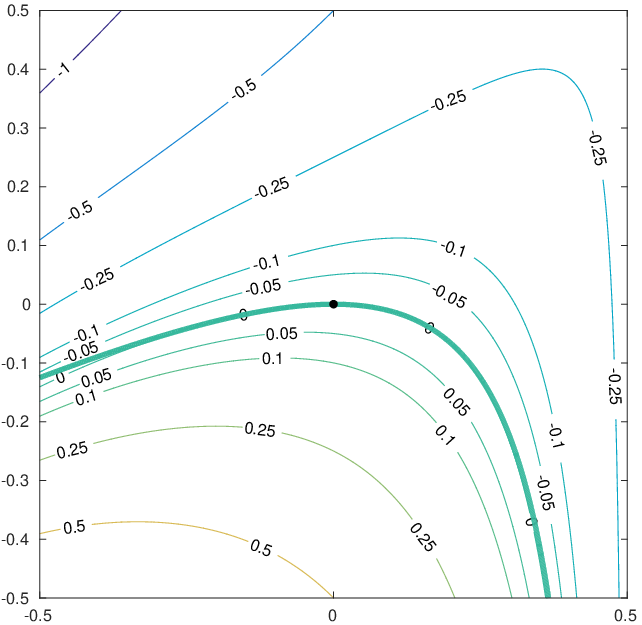
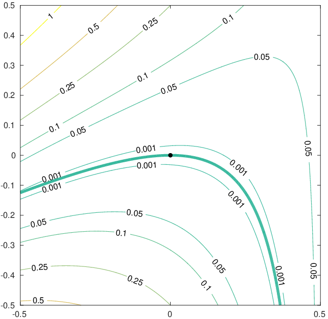
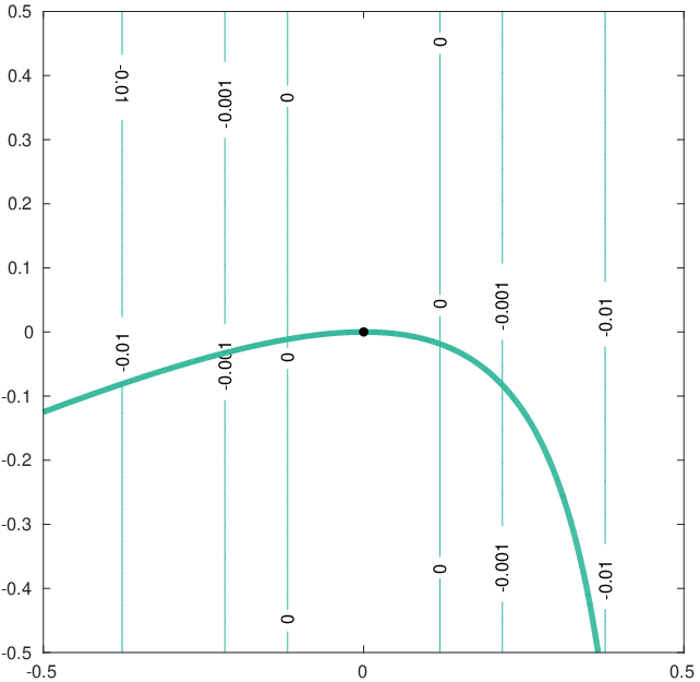
It is worthwhile to note that the above discussion has wider implications. Indeed the first of the problematic terms in (38) not only occurs in the function $\mu(x,t)$ used in this paper, but also when applying to problem (1) a quadratic, $\ell_{1}$ or $\ell_{\infty}$ penalty function, a classical augmented Lagrangian approach, or a sequential quadratic programming method using a merit function depending on such penalty terms. The same difficulty may also occur if more general penalizations of the type $p(\nu(x))$ (for some increasing smooth function $p$ from $\Re^{+}$ to $\Re^{+}$ ) are employed. Indeed, consider the derivatives of $p(\nu(x))$ . One verifies that

\begin{array}[]{lcl}\nabla_{x}^{4}p(\nu(x))&=&p^{\prime\prime\prime\prime}(\nu(x))[\nabla_{x}^{1}\nu(x)]^{4\otimes}+6p^{\prime\prime\prime}(\nu(x))\nabla_{x}^{2}\nu(x)\otimes[\nabla_{x}^{1}\nu(x)]^{2\otimes}\\[8.61108pt] &&+4p^{\prime\prime}(\nu(x))\nabla_{x}^{3}\nu(x)\otimes\nabla_{x}^{1}\nu(x)+3p^{\prime\prime}(\nu(x))[\nabla_{x}^{2}\nu(x)]^{2\otimes}\\[8.61108pt] &&+p^{\prime}(\nu(x))\nabla_{x}^{4}\nu(x)\\[12.91663pt] \end{array}

whose last term, together with

\nabla_{x}^{4}\nu(x)=\sum_{i=1}^{m}\Bigg[4\,\nabla_{x}^{3}c_{i}(x)\otimes\nabla_{x}^{1}c_{i}(x)+3\,[\nabla_{x}^{2}c_{i}(x)]^{2\otimes}+c_{i}(x)\nabla_{x}^{4}c_{i}(x)\Bigg],

indicates that the troublesome terms involving $[\nabla_{x}^{2}c_{i}(x)]^{2\otimes}$ do not vanish unless $p^{\prime}(\nu(x))$ also vanishes with $\nu(x)$ .

None of the linear or quadratic penalization approaches can therefore be expected to reliably produce critical points of orders four or more. Innovative techniques are thus needed if one is interested to compute high-order critical points of (1) of higher order. One possible research direction is to follow the propositions formulated in [18] and to exploit penalization terms of order higher than two in the definitions of $\nu$ and $\mu$ , for which an improved evaluation complexity bound is already available for the subproblem solution.

5 Conclusions and discussion

We have formulated and analyzed, in Section 2, the necessary conditions for high-order optimality in nonlinear optimization problems involving both convex set constraints and nonlinear equalities. We have also discussed the difficulties inherent to their form for third-order critical points and higher.

We then have shown in Sections 3 and 4 that the evaluation complexity of finding an approximate $q$ -th-order scaled critical point ( $q=1,2,3$ ) for a large class of smooth nonlinear optimization problem involving both equality and inequality constraints is at most $O(\epsilon_{\mbox{\tiny P}}^{1-\pi}\epsilon_{\mbox{\tiny D}}^{-\pi})$ evaluations of the objective function, constraints and their derivatives, where $\epsilon^{\pi}$ is the order of the guaranteed objective function decrease during the successful iterations of an underlying inner algorithm for convexly constrained least-squares problems. We refer here to an “approximate scaled critical point” in that such a point is required to satisfy (9) or (10), where the accuracy is scaled by the size of the constraint violation or that of the Lagrange multipliers. In particular, the above results provide the first evaluation complexity bound for second- and third-order criticality in the case involving general inequality and equality constraints.

This result also corrects an unfortunate error⁶⁶ 6 The second equality in the first equation of Lemma 3.4 in [21] only holds if one is ready to flip the gradient’s sign if necessary. in the first-order analysis of [21], that allows a vector of Lagrange multipliers whose sign is arbitrary (in line with a purely first-order setting where minimization and maximization are not distinguished). The present analysis now yields the multiplier with the sign associated with minimization.

Interestingly, an $O(\epsilon_{\mbox{\tiny P}}\epsilon_{\mbox{\tiny D}}^{-(p+1)/p}\min[\epsilon_{\mbox{\tiny D}},\epsilon_{\mbox{\tiny P}}]^{-(p+1)/p})$ evaluation complexity bound was also proved by Birgin, Gardenghi, Martínez, Santos and Toint in [6] for first-order unscaled, standard KKT conditions and in the least expensive of three cases depending on the degree of degeneracy identifiable by the algorithm⁷⁷ 7 This result also assumes boundedness of $f(x_{1})$ .. Even if the bounds for the scaled and unscaled cases coincide in order when $\epsilon_{\mbox{\tiny P}}\leq\epsilon_{\mbox{\tiny D}}$ , comparing the two results for first-order critical points is not straightforward. On one hand the scaled conditions take into account the possibly different scaling of the objective function and constraints. On the other hand the same scaled conditions may result in earlier termination with (10) if the Lagrange multipliers are very large, as (10) is then consistent with the weaker requirement of finding a John’s point. But the framework discussed in the present paper also differs from that of [6] in additional significant ways. The first is that second-order critical points are now covered in the analysis. If we now restrict the scope to first-order, the present paper provides a potentially stronger version of the termination of the algorithm at infeasible points (in Phase 1): indeed the second part of (9) can be interpreted as requiring that the size of the feasible gradient of $\|c(x)\|$ is below $\epsilon_{\mbox{\tiny D}}$ , while [6] considers the gradient of $\|c(x)\|^{2}$ instead. The second is that, if termination occurs in Phase 2 for an $x_{\epsilon}$ such that $\phi_{\nu,1}^{\Delta_{k}}(x_{\epsilon})$ is of order $\epsilon_{\mbox{\tiny P}}\epsilon_{\mbox{\tiny D}}\Delta_{k}$ (thereby covering the case where $f(x_{\epsilon})=t_{k}$ discussed in Theorem 4.5) and $x_{\epsilon}\in{\cal F}^{0}$ , then $\|P_{{\cal T}_{*}}[-\nabla_{x}^{1}\nu(x_{*})]\|=\|\nabla_{x}^{1}\nu(x_{*})\|$ is of the same order and Birgin et al. show that, in this case, the Łojaciewicz inequality [43] must fail for $c$ in the limit for $\epsilon_{\mbox{\tiny P}}$ and $\epsilon_{\mbox{\tiny D}}$ tending to zero (see [6] for details). This observation is interesting because smooth functions satisfy the Łojaciewicz inequality under relatively weak conditions, implying that termination in these circumstances is unlikely. The same information is also obtained in [6], albeit at the price of worsening the evaluation complexity bound mentioned above by an order of magnitude in $\epsilon_{\mbox{\tiny D}}$ . We also note that the approach of [6] requires the minimization, at each iteration, of a residual whose second derivatives are discontinuous, while all functions used in the present paper are $p$ times continuously differentiable. A final difference between the two approaches is obviously our introduction of $\phi_{\mu,j}^{\Delta_{k}}$ in the expression of the criticality condition in Theorem 4.5 for taking the inequality constraints into account.

Will regularization-based methods provide better evaluation complexity bounds when using polynomial models of higher order? Can the limitations of penalty approaches for finding high-order solutions for equality constrained problems be circumvented? These and many other questions remain open at this stage.

Acknowledgements

The authors would like to thank Oliver Stein for suggesting reference [41]. The work of the second author was supported by EPSRC grant EP/M025179/1. The third author acknowleges the support provided by the Belgian Fund for Scientific Research (FNRS), the Leverhulme Trust (UK), Balliol College (Oxford, UK), the Department of Applied Mathematics of the Hong Kong Polytechnic University, ENSEEIHT (Toulouse, France) and INDAM (Florence, Italy).

References

[1] A. Anandkumar and R. Ge. Efficient approaches for escaping high-order saddle points in nonconvex optimization. arXiv.1602.05908, 2016.
[2] E. Bergou, Y. Diouane, and S. Gratton. On the use of the energy norm in trust-region and adaptive cubic regularization subproblems. Technical Report, 2017.
[3] W. Bian and X. Chen. Worst-case complexity of smoothing quadratic regularization methods for non-Lipschitzian optimization. SIAM Journal on Optimization 23 (2013), 1718–1741.
[4] W. Bian and X. Chen. Linearly constrained non-Lipschitzian optimization for image restoration. Technical report, Department of Applied Mathematics, Polytechnic University of Hong Kong, Hong Kong, 2015.
[5] W. Bian, X. Chen, and Y. Ye. Complexity analysis of interior point algorithms for non-Lipschitz and nonconvex minimization. Mathematical Programming, Series A 149 (2015), 301–327.
[6] E. G. Birgin, J. L. Gardenghi, J. M. Martínez, S. A. Santos, and Ph. L. Toint. Evaluation complexity for nonlinear constrained optimization using unscaled KKT conditions and high-order models. SIAM Journal on Optimization 26 (2016), 951–967.
[7] E. G. Birgin, J. L. Gardenghi, J. M. Martínez, S. A. Santos, and Ph. L. Toint. Worst-case evaluation complexity for unconstrained nonlinear optimization using high-order regularized models. Mathematical Programming, Series A DOI: 10.1007/s10107-016-1065-8.
[8] N. Boumal, P.-A. Absil, and C. Cartis. Global rates of convergence for nonconvex optimization on manifolds. Technical Report Technical Report arXiv:1605.08101, Oxford University, Oxford, UK, 2016.
[9] O. A. Brezhneva and A. Tret’yakov. Optimality conditions for degenerate extremum problems with equality constraints. SIAM Journal on Control and Optimization 42(2003), 729–743.
[10] O. A. Brezhneva and A. Tret’yakov. The $p$ th-order optimality conditions for inequality constrained optimization problems. Nonlinear Analysis 63 (2005), 1357–1366.
[11] C. Cartis, N. I. M. Gould, and Ph. L. Toint. On the complexity of steepest descent, Newton’s and regularized Newton’s methods for nonconvex unconstrained optimization. SIAM Journal on Optimization 20 (2010), 2833–2852.
[12] C. Cartis, N. I. M. Gould, and Ph. L. Toint. Adaptive cubic regularization methods for unconstrained optimization. Part I: motivation, convergence and numerical results. Mathematical Programming, Series A 127(2011), 245–295.
[13] C. Cartis, N. I. M. Gould, and Ph. L. Toint. Adaptive cubic regularization methods for unconstrained optimization. Part II: worst-case function-evaluation complexity. Mathematical Programming, Series A 130 (2011), 295–319.
[14] C. Cartis, N. I. M. Gould, and Ph. L. Toint. An adaptive cubic regularization algorithm for nonconvex optimization with convex constraints and its function-evaluation complexity. IMA Journal of Numerical Analysis 32 (2012), 1662–1695.
[15] C. Cartis, N. I. M. Gould, and Ph. L. Toint. On the evaluation complexity of cubic regularization methods for potentially rank-deficient nonlinear least-squares problems and its relevance to constrained nonlinear optimization. SIAM Journal on Optimization, 23(3):1553–-1574, 2013.
[16] C. Cartis, N. I. M. Gould, and Ph. L. Toint. Evaluation complexity bounds for smooth constrained nonlinear optimization using scaled KKT conditions and high-order models. Technical Report 1912, Mathematical Institute E-prints Archive, University of Oxford, 2015.
[17] C. Cartis, N. I. M. Gould, and Ph. L. Toint. Evaluation complexity bounds for smooth constrained nonlinear optimization using scaled KKT conditions, high-order models and the $\chi$ criticality measure. arXiv:1705.04895, 2015.
[18] C. Cartis, N. I. M. Gould, and Ph. L. Toint. Improved worst-case evaluation complexity for potentially rank-deficient nonlinear least-euclidean-norm problems using higher-order regularized models. Technical Report 1915, Mathematical Institute E-prints Archive, University of Oxford, 2015.
[19] C. Cartis, N. I. M. Gould, and Ph. L. Toint. Second-order optimality and beyond: characterization and evaluation complexity in convexly-constrained nonlinear optimization. Foundations of Computational Mathematics, 2017 (online first).
[20] C. Cartis, N. I. M. Gould, and Ph. L. Toint. On the complexity of finding first-order critical points in constrained nonlinear optimization. Mathematical Programming, Series A 144, 93–106, 2013.
[21] C. Cartis, N. I. M. Gould, and Ph. L. Toint. On the evaluation complexity of constrained nonlinear least-squares and general constrained nonlinear optimization using second-order methods. SIAM Journal on Numerical Analysis 53, 836–851, 2015.
[22] C. Cartis, Ph. R. Sampaio, and Ph. L. Toint. Worst-case complexity of first-order non-monotone gradient-related algorithms for unconstrained optimization. Optimization 64, 1349–1361, 2015.
[23] C. Cartis and K. Scheinberg. Global convergence rate analysis of unconstrained optimization methods based on probabilistic models. Mathematical Programming, Series A DOI: 10.1007/s10107-017-1137-4.
[24] X. Chen, Ph. L. Toint, and H. Wang. Partially separable convexly-constrained optimization with non-Lipschitzian singularities and its complexity. arXiv:1704.06919, 2017.
[25] A. R. Conn, N. I. M. Gould, and Ph. L. Toint. Trust-Region Methods. MPS-SIAM Series on Optimization. SIAM, Philadelphia, USA, 2000.
[26] F. E. Curtis, D. P. Robinson, and M. Samadi. Complexity analysis of a trust funnel algorithm for equality constrained optimization. Technical Report 16T-03, ISE/COR@L, LeHigh University, Bethlehem, PA, USA, 2017.
[27] F. E. Curtis, D. P. Robinson, and M. Samadi. A trust-region algorithm with a worst-case iteration complexity of $O(\epsilon^{-3/2})$ for nonconvex optimization. Mathematical Programming, Series A 162 (2017), 1–32.
[28] M. Dodangeh, L. N. Vicente, and Z. Zhang. On the optimal order of worst case complexity of direct search. Optimization Letters 10 (2016), 699–708.
[29] J. P. Dussault. ARC_q: a new adaptive regularization by cubics. Optimization Methods and Software DOI:10.1080/10556788.2017.1322080
[30] R. Garmanjani, D. Júdice, and L. N. Vicente. Trust-region methods without using derivatives: Worst case complexity and the non-smooth case. Technical Report 15-03, Department of mathematics, University of Coimbra, Coimbra, Portugal, 2015.
[31] D. Ge, X. Jiang, and Y. Ye. A note on the complexity of ${L}_{p}$ minimization. Mathematical Programming, Series A 21 (2011), 1721–1739.
[32] S. Ghadimi and G. Lan. Accelerated gradient methods for nonconvex nonlinear and stochastic programming. Mathematical Programming, Series A, 156 (2016), 59–100.
[33] G. N. Grapiglia and Yu. Nesterov. Regularized Newton methods for minimizing Ffnctions with Hölder continuous Hessians. SIAM Journal on Optimization, 27(1), 478–506, 2017.
[34] G. N. Grapiglia, J. Yuan, and Y. Yuan. Nonlinear stepsize control algorithms: Complexity bounds for first and second-order optimality. Technical report, Departamento de mathematica, Universidade Federal do Paraná, Centro Politécnico, Curitiba, Paraná, Brazil, 2015.
[35] G. N. Grapiglia, J. Yuan, and Y. Yuan. On the convergence and worst-case complexity of trust-region and regularization methods for unconstrained optimization. Mathematical Programming, Series A 152 (2015), 491–520.
[36] S. Gratton, C. W. Royer, and L. N. Vicente. A decoupled first/second-order steps technique for nonconvex nonlinear unconstrained optimization with improved complexity bounds. Technical Report TR 17-21, Department of Mathematics, University of Coimbra, Coimbra, Portugal, 2017.
[37] S. Gratton, C. W. Royer, L. N. Vicente, and Z. Zhang. Direct search based on probabilistic descent. SIAM Journal on Optimization 25 (2015), 1515–1541.
[38] S. Gratton, A. Sartenaer, and Ph. L. Toint. Recursive trust-region methods for multiscale nonlinear optimization. SIAM Journal on Optimization, 19 (2008), 414–444.
[39] H. Hancock. The Theory of Maxima and Minima. The Athenaeum Press, Ginn & Co, NewYork, USA, 1917. Available on line at https://archive.org/details/theoryofmaximami00hancuoft.
[40] J.-B. Hiriart-Urruty and C. Lemaréchal. Convex Analysis and Minimization Algorithms. Part 1: Fundamentals. Springer Verlag, Heidelberg, Berlin, New York, 1993.
[41] W. Hogan. Point-to-set maps in mathematical programming. SIAM Review 15 (1973), 591–603.
[42] F. Jarre. On Nesterov’s smooth Chebyshev-Rosenbrock function. Optimization Methods and Software 28 (2013), 478–500.
[43] S. Lojasiewicz. Ensembles semi-analytiques. Technical report, Institut des Hautes Etudes Scientifiques, Bures-sur-Yvette, France, 1965. Available online at http://perso.univ- rennes1.fr/michel.coste/Lojasiewicz.pdf.
[44] S. Lu, Z. Wei, and L. Li. A trust-region algorithm with adaptive cubic regularization methods for nonsmooth convex minimization. Computational Optimization and Applications 51 (2012), 551–573.
[45] J. M. Martínez. On high-order model regularization for constrained optimization. Technical report, Department of Applied Mathematics, IMECC-UNICAMP, Campinas, Brasil, February 2017.
[46] J. M. Martínez and M. Raydan. Cubic-regularization counterpart of a variable-norm trust-region method for unconstrained minimization. Journal of Global Optimization, 2016, DOI:10.1007/s10898-016-0475-8.
[47] J. J. Moreau. Décomposition orthogonale d’un espace hilbertien selon deux cônes mutuellement polaires. Comptes-Rendus de l’Académie des Sciences (Paris) 255 (1962), 238–240.
[48] Yu. Nesterov and B. T. Polyak. Cubic regularization of Newton method and its global performance. Mathematical Programming, Series A 108 (2006), 177–205.
[49] R. T. Rockafellar. Convex Analyis. Princeton University Press, Princeton, USA, 1970.
[50] K. Scheinberg and X. Tang. Complexity in inexact proximal Newton methods. Technical report, Lehigh University, Bethlehem, USA, 2014.
[51] K. Ueda and N. Yamashita. Convergence properties of the regularized Newton method for the unconstrained nonconvex optimization. Applied Mathematics & Optimization 62 (2010), 27–46.
[52] K. Ueda and N. Yamashita. On a global complexity bound of the Levenberg-Marquardt method. Journal of Optimization Theory and Applications 147 (2010), 443–453.
[53] L. N. Vicente. Worst case complexity of direct search. EURO Journal on Computational Optimization 1 (2013), 143–153.

Appendix

Details of the derivation of (15)

For the trust-region algorithm,

f(x_{1}^{*})\leq f(x_{1})+\left(\displaystyle\max_{\xi\in\cup_{j\in{\cal S}}[x_{j},x_{j+1}]}\|\nabla_{x}^{1}\nu(\xi)\|\right)\Delta_{\max}\left(\left\lfloor\kappa_{\mbox{\rm\tiny CC}}^{\|c\|}\|c(x_{1})\|\,\epsilon_{\mbox{\tiny P}}^{-q}\epsilon_{\mbox{\tiny D}}^{-(q+1)}\right\rfloor+1\right).

For the regularization algorithm,

\begin{array}[]{lcl}f(x_{1})&\leq&f(x_{0})+\left(\frac{\displaystyle\nu(x_{0})(p+1)!}{\displaystyle\eta\sigma_{\min}}\right)^{\frac{1}{p+1}}\times\\[4.30554pt] &&\displaystyle\max_{\xi\in\cup_{j\in{\cal S}}[x_{j},x_{j+1}]}\|\nabla_{x}^{1}\nu(\xi)\|\left\{\left\lfloor\kappa_{\mbox{\rm\tiny CC}}^{\|c\|}\|c(x_{0})\|\,\displaystyle\max\left[\epsilon_{\mbox{\tiny P}}^{-1},\epsilon_{\mbox{\tiny P}}^{-\frac{1}{p}}\epsilon_{\mbox{\tiny D}}^{-\frac{p+1}{p+1-q}}\right]\right\rfloor+1\right\}.\end{array}

Details for the example (39)

We prove the validity of the statement made after the definition of problem (39), namely that $\mu(0,t_{\epsilon})$ satisfies the necessary conditions for a fourth order minimizer at the origin while the problem itself has a global (fourth order) constrained maximizer.

Let $T_{3}(x)=x_{2}+x_{1}^{2}-2x_{1}x_{2}$ and define, for some $\varepsilon\in(0,1]$ ,

f(x)=-T_{3}(x)-{\scriptstyle\frac{1}{2}}x_{1}^{4}\;\;\mbox{ and }\;\;c(x)=\varepsilon+T_{3}(x).

(A.1)

and thus, for a given multiplier $y$ ,

\Lambda(x,y)=-T_{3}(x)-{\scriptstyle\frac{1}{2}}x_{1}^{4}+y[\varepsilon+T_{3}(x)]

(A.2)

We have that

\nabla_{x}^{1}T_{3}(x)=\left(\begin{array}[]{c}2x_{1}-2x_{2}\\ 1-2x_{1}\end{array}\right),\;\;\;\;\nabla_{x}^{2}T_{3}(x)=\left(\begin{array}[]{rr}2&-2\\ -2&0\end{array}\right)\;\;\mbox{and}\;\;\nabla_{x}^{3}T_{3}(x)=0.

(A.3)

Thus, at the origin and for $t_{\epsilon}=-\varepsilon$

c(0)=\varepsilon=f(0)-t_{\epsilon}\;\;\mbox{ and }\;\;\nabla_{x}^{j}c(0)=\nabla_{x}^{j}T_{3}(0)=-\nabla_{x}^{j}f(0)\;\;\mbox{ for }\;\;j=1,2,3.

(A.4)

As a consequence, the choice $y=1$ , (A.2) and (A.3) ensure that $\Lambda(x,1)=\varepsilon-{\scriptstyle\frac{1}{2}}x_{1}^{4}$ as well as

\nabla_{x}^{1}\Lambda(0,1)=0,\;\;\;\;\nabla_{x}^{2}\Lambda(0,1)=0,\;\;\;\;\nabla_{x}^{3}\Lambda(0,1)=0,\;\;\;\;\nabla_{x}^{4}\Lambda(0,1)=\nabla_{x}^{4}f(0)=-12e_{1}^{\otimes 4}.

(A.5)

Using (16)-(19) and (A.4), we also have that, for $t=-\varepsilon$ ,

\nabla_{x}^{1}\mu(0,t_{\epsilon})=(c(0)-f(0)+t_{\epsilon})\nabla_{x}^{1}T_{3}(0)=(\varepsilon-0-\varepsilon)e_{2}=0,

(A.6)

\nabla_{x}^{2}\mu(0,t_{\epsilon})=2\,\nabla_{x}^{1}T_{3}(0)\otimes\nabla_{x}^{1}T_{3}(0)=2e_{2}e_{2}^{T},\;\;\;\;\nabla_{x}^{3}\mu(0,t_{\epsilon})=6\,\nabla_{x}^{2}T_{3}(0)\otimes\nabla_{x}^{1}T_{3}(0)=0

(A.7)

and, using the last equation in (A.5),

\begin{array}[]{lcl}\nabla_{x}^{4}\mu(0,t_{\epsilon})&=&6\,\nabla_{x}^{2}T_{3}(0)\otimes\nabla_{x}^{2}T_{3}(0)+c(0)\nabla_{x}^{4}c(0)+(f(0)-t_{\epsilon})\nabla_{x}^{4}f(0)\\[4.30554pt] &=&12\left[\left(\begin{array}[]{rr}1&-1\\ -1&0\end{array}\right)^{\otimes 2}-\varepsilon e_{1}^{\otimes 4}\right].\end{array}

(A.8)

(Notice the contribution of the first term in the bracketed expression, potentially dwarfing that of the second for sufficiently small $\epsilon$ .)

Let us attempt to verify (15)-(9) with $q=4$ for the problem of minimizing $\mu(x,t_{\epsilon})$ with $s_{1}\in\ker^{2}[\nabla^{2}\mu]=\mbox{span}\left\{e_{1}\right\}$ . We have that (15) holds because of (A.6). We also obtain, from (A.6)-(A.8), that, for $s_{1}=\tau e_{1}$ for some $\tau\in\Re$ and for any choice of $s_{2},s_{3},s_{4}\in\Re^{n}$ ,

\nabla_{x}^{2}\mu(0,t_{\epsilon})[s_{2}]+{\scriptstyle\frac{1}{2}}\nabla_{x}^{2}\mu(0,t_{\epsilon})[s_{1}]^{2}=0^{T}s_{2}+\tau e_{2}e_{2}^{T}e_{1}=0,

\nabla_{x}^{3}\mu(0,t_{\epsilon})[s_{3}]+\tau\nabla_{x}^{2}\mu(0,t_{\epsilon})[s_{1},s_{2}]+\frac{\tau^{3}}{6}\nabla_{x}^{3}\mu(0,t_{\epsilon})[s_{1}]^{3}=0^{T}s_{3}+\tau s_{2}^{T}e_{2}e_{2}^{T}e_{1}+\frac{\tau^{3}}{6}0[s_{1}]^{3}=0

and

\begin{array}[]{ll}\nabla_{x}^{1}&\!\!\!\!\!\mu(0,t_{\epsilon})[s_{4}]+\nabla_{x}^{2}\mu(0,t_{\epsilon})[s_{1},s_{3}]+{\scriptstyle\frac{1}{2}}\nabla_{x}^{2}\mu(0,t_{\epsilon})[s_{2}]^{2}+{\scriptstyle\frac{1}{2}}\nabla_{x}^{3}\mu(0,t_{\epsilon})[s_{1},s_{1},s_{2}]+{\scriptstyle\frac{1}{24}}\nabla_{x}^{4}\mu(0,t_{\epsilon})[s_{1}]^{4}\\[6.45831pt] &=0^{T}s_{4}++\tau s_{3}^{T}e_{2}e_{2}^{T}e_{1}+{\scriptstyle\frac{1}{2}}(e_{2}^{T}s_{2})^{2}+\frac{\tau^{2}}{2}0^{T}[e_{1},e_{1},s_{2}]\\[6.45831pt] &\;\;\;\;\;\;\;\;\;\;\;\;+{\scriptstyle\frac{12}{24}}\left[\left\|e_{1}^{T}\left(\begin{array}[]{rr}1&-1\\ -1&0\end{array}\right)e_{1}\right\|^{2}-\varepsilon\right]\tau^{4}(e_{1}^{T}e_{1})^{4}\\[10.76385pt] &={\scriptstyle\frac{1}{2}}(e_{2}^{T}s_{2})^{2}+{\scriptstyle\frac{1}{2}}(1-\varepsilon)\tau^{4}(e_{1}^{T}e_{1})^{4}.\end{array}

(A.9)

The choice of $s_{2}$ , $s_{3}$ and $s_{4}$ is however constrained by (9) for $i=1,2,3$ , in that those vector must also satisfy the equations

\nabla_{x}^{1}c(0)[s_{1}]=0=\tau e_{2}^{T}e_{1},

\nabla_{x}^{1}c(0)[s_{2}]+{\scriptstyle\frac{1}{2}}\nabla_{x}^{2}c(0)[s_{1}]^{2}=0=e_{2}^{T}s_{2}+\tau^{2}e_{1}^{T}\left(\begin{array}[]{rr}1&-1\\ -1&0\end{array}\right)e_{1},

\nabla_{x}^{1}c(0)[s_{3}]+\nabla_{x}^{2}c(0)[s_{1},s_{2}]+{\scriptstyle\frac{1}{2}}\nabla_{x}^{3}c(0)[s_{1}]^{3}=0=e_{2}^{T}s_{3}+2\tau(e_{1}-e_{2})^{T}s_{2}+\tau^{3}0^{T}[e_{1}]^{3}.

and

\begin{array}[]{ll}\nabla_{x}^{1}&\!\!\!\!\!c(0)[s_{4}]+\nabla_{x}^{2}c(0)[s_{1},s_{3}]++{\scriptstyle\frac{1}{2}}\nabla_{x}^{2}c(0)[s_{2}]^{2}+{\scriptstyle\frac{1}{2}}\nabla_{x}^{3}c(0)[s_{1},s_{1},s_{2}]^{2}+{\scriptstyle\frac{1}{24}}\nabla_{x}^{4}c(0)[s_{1}]^{4}\\[4.30554pt] &=0=e_{2}^{T}s_{4}+e_{1}^{T}s_{2}(e_{1}^{T}s_{2}-2\tau^{2})+2\tau e_{1}^{T}s_{3}-4\tau^{2}.\end{array}

The second, third and fourth of these conditions impose constraints on the values of $e_{2}^{T}s_{2}$ , $e_{2}^{T}s_{3}$ and $e_{2}^{T}s_{4}$ . In particular, the second implies that $e_{2}^{T}s_{2}=-\tau^{2}$ , which we may then substitute in (A.9) and deduce that

\begin{array}[]{ll}\nabla_{x}^{4}&\!\!\!\!\!\mu(0,t_{\epsilon})[s_{4}]+\nabla_{x}^{2}\mu(0,t_{\epsilon})[s_{1},s_{3}]+{\scriptstyle\frac{1}{2}}\nabla_{x}^{2}\mu(0,t_{\epsilon})[s_{2}]^{2}+{\scriptstyle\frac{1}{2}}\nabla_{x}^{3}\mu(0,t_{\epsilon})[s_{1},s_{1},s_{2}]+{\scriptstyle\frac{1}{24}}\nabla_{x}^{4}\mu(0,t_{\epsilon})[s_{1}]^{4}\\[6.45831pt] &={\scriptstyle\frac{1}{2}}\tau^{4}+({\scriptstyle\frac{1}{2}}-\varepsilon)\tau^{4}=(1-{\scriptstyle\frac{1}{2}}\varepsilon)\tau^{4}\geq 0.\end{array}

(A.10)

We therefore obtain that, for all $\varepsilon\in(0,1]$ , $x_{*}$ satisfies the necessary conditions of Theorem 2.1 with $q=4$ , except that $c(x_{*})=\varepsilon$ . However (A.5) shows that $\Lambda(x,y_{\epsilon})$ is a polynomial of degree 4 with a global maximizer at the origin, independently of the value of $\varepsilon$ . Letting $\varepsilon$ tend to zero and using the fact that all quantities in the example depend continuously on this parameter then allows to conclude.

Optimality of orders one to three and beyond: characterization and evaluation complexity in constrained nonconvex optimization

Abstract

1 Introduction

2 Necessary optimality conditions for constrained optimization

Theorem 2.1

Corollary 2.2

3 A minimization algorithm

3.1 Inner algorithms for constrained least-squares problems

3.2 The outer algorithm

Lemma 3.1

4 Evaluation complexity

Lemma 4.1

Lemma 4.2

Lemma 4.3

Lemma 4.4

Theorem 4.5

Theorem 4.6

Theorem 4.7

4.1 Beyond third-order optimality?

5 Conclusions and discussion

Acknowledgements

References

Details of the derivation of (15)

Details for the example (39)

Optimality of orders one to three and beyond:
characterization and evaluation complexity
in constrained nonconvex optimization