Stability of new exact solutions of the nonlinear Schrödinger equation in a Pöschl-Teller external potential

The study of open systems with balanced loss and gain, typically defined by Parity-Time ($\mathcal{PT}$) symmetry, has elicited significant attention from physics, nonlinear science and mathematics communities during the past decade. This is in part due to their emerging applications in many physical contexts and in part due to their intriguing mathematical structure. The initial investigation of such systems [2, 3, 4, 5] arose in the context of whether non-Hermitician quantum systems could lead to entirely real eigenvalues. Keeping in perspective the formal similarity of the Schrödinger equation with Maxwell’s equations in the paraxial approximation, many experimentalists realized that such $\mathcal{PT}$-invariant systems can indeed be fabricated using optical means [6, 7, 8, 9, 10, 11, 12, 13, 14, 15]. Motivated by this success, in the ensuing years, $\mathcal{PT}$-invariant phenomena was also observed in electronic circuits [16, 17], mechanical constructs [18], whispering-gallery microcavities [19], among many other physical systems.

In a parallel development, the concept of supersymmetry (SUSY) prevalent in high-energy physics was also experimentally studied in optics [20, 21]. The underlying notion is that for a given potential we can obtain a SUSY partner potential such that both potentials possess identical spectrum (with possibly one eigenvalue different) [22, 23]. A simultaneous presence of $\mathcal{PT}$-symmetry and SUSY can lead to unexpected phenomena and is likely to be very useful in achieving transparent and one-way reflectionless complex optical potentials [24, 25, 26, 27, 28]. Previously [1] we studied the interplay between nonlinearity, $\mathcal{PT}$-symmetry and supersymmetry as well as the rich consequences of this interplay. There we obtained exact solutions of the general nonlinear Schrödinger equation (NLSE) in 1+1 dimensions in the presence of a $\mathcal{PT}$-symmetric complex potential [22, 29]. In a recent paper [30] we studied the stability properties of the solutions of NLSE in the real partner potential of the problem studied in [1] which was a Pöschl-Teller potential [31, 32].

Here our objective is to discuss the stability properties of two related exact solutions which exist when we change the sign of the nonlinear coupling $g$ to being negative keeping the potential attractive, or keep the sign of the nonlinear term unchanged but consider a repulsive potential. In the latter case we will find that the solutions are translationally unstable, whereas in the former case the solutions are stable to small perturbations

The time-dependent version of the variational approximation can be traced to an obscure appendix in the 1930 Russian edition of the ‘‘Principles of Wave Mechanics,’’ by Dirac.¹¹ 1 P. A. M. Dirac, Appendix to the Russian edition of The Principles of Wave Mechanics, as cited by Ia. I. Frenkel, Wave Mechanics, Advanced General Theory (Clarendon Press, Oxford, 1934), pp. 253, 436. Pattanayak and Schieve [33] point out that the reference often quoted, P. A. M. Dirac, Proc. Cambridge Philos. Soc. 26, 376 (1930), does not contain this equation. In this version of the variational approximation, the wave function is taken to be a function of a number of time-dependent parameters. Variation of the action, as defined by Dirac, leads to a classical set of Hamiltonian equations of motion for the parameters. These classical equations are then solved as a function of time to provide an approximation to the evolution of the wave function.

The action which leads to Eq. (47) is given by

$$\Gamma[\psi,\psi^{\ast}]=\!\int\!\differential{t}L[\psi,\psi^{\ast}]$$

(11)

where

	$\displaystyle L[\psi,\psi^{\ast}]$	$\displaystyle=\frac{{\rm i}}{2}\!\int\!\differential{x}\quantity[\, \psi^{\ast} (\partial_t \psi) - (\partial_t \psi^{\ast} ) \psi\,]-H[\psi,\psi^{\ast}]\>,$		(12a)
	$\displaystyle H[\psi,\psi^{\ast}]$	$\displaystyle=\!\int\!\differential{x}\bigl[\,\absolutevalue{\partial_x \psi}^{2}-\frac{g\,\absolutevalue{\psi}^{2\kappa+2}}{\kappa+1}+V(x)\,\absolutevalue{\psi}^{2}\,\bigr]\>.$		(12b)

The NLSE and its complex conjugate follow from minimizing the action via,

$$\frac{\delta\Gamma}{\delta\psi^{\ast}}=\frac{\delta\Gamma}{\delta\psi}=0\>.$$

(13)

Derrick’s theorem [34] states that for a Hamiltonian dynamical system, an exact solution of the equation of motion is unstable if under a scale transformation, $x\mapsto\beta x$ with fixed normalization, the energy of the system is lowered. The stretched wave function for Derrick’s theorem is given by

$$\psi_{\beta}(x,t)=A(\tilde{b},\beta,\gamma)\,\sech^{\gamma}(\beta x)\>,$$

(25)

with the normalization fixed by the requirement,

	$\displaystyle M[\tilde{b},\beta,\gamma]$	$\displaystyle=\!\int\!\differential{x}\absolutevalue{\psi_{\beta}(x,t)}^{2}=A^{2}(\tilde{b},\beta,\gamma)\,c_{1}[\gamma]/\beta$		(26)
		$\displaystyle=M_{0}[\tilde{b},\gamma]=A_{0}^{2}(\tilde{b},\gamma)\,c_{1}[\gamma]\>.$

So $A^{2}(\tilde{b},\beta,\gamma)=\beta A_{0}^{2}(\tilde{b},\gamma)$. Evaluation of the Hamiltonian (12b) with Derrick’s wave function gives:

$$H(\beta,\gamma)=H_{1}(\beta,\gamma)+H_{2}(\beta,\gamma)+H_{3}(\beta,\gamma)\>,$$

(27)

where

	$\displaystyle H_{1}(\beta,\gamma)$	$\displaystyle=\!\int\!\differential{x}\absolutevalue{\partial_x \psi_{\beta}}^{2}$		(28a)
		$\displaystyle=A_{0}^{2}\,\beta^{2}\gamma^{2}\!\int\!\differential{z}\sech^{2\gamma+2}(z)\sinh^{2}(z)$
		$\displaystyle=\frac{A_{0}^{2}\,\beta^{2}\,\gamma}{2}\,c_{1}[\gamma+1]\>,$
	$\displaystyle H_{2}(\beta,\gamma)$	$\displaystyle=-\frac{g}{\kappa+1}\!\int\!\differential{x}\absolutevalue{\psi_{\beta}}^{2\kappa+2}$		(28b)
		$\displaystyle=-g\,A_{0}^{2/\gamma}\,A_{0}^{2}\,\frac{\gamma\,\beta^{1/\gamma}}{\gamma+1}\!\int\!\differential{z}\sech^{2\gamma+2}(z)\>,$
		$\displaystyle=-A_{0}^{2}\,\frac{\gamma\,\beta^{1/\gamma}}{\gamma+1}\,[\,\gamma(\gamma+1)-\lambda\,\tilde{b}^{2}\,]\,c_{1}[\gamma+1]\>,$
	$\displaystyle H_{3}(\beta,\gamma)$	$\displaystyle=\!\int\!\differential{x}V(x)\,\absolutevalue{\psi_{\beta}}^{2}$		(28c)
		$\displaystyle=-\lambda\,\tilde{b}^{2}\,A_{0}^{2}\,\beta\!\int\!\differential{x}\sech^{2}(x)\sech^{2\gamma}(\beta x)$
		$\displaystyle=-\lambda\,\tilde{b}^{2}\,A_{0}^{2}\,g_{1}[\beta,\gamma]\>,$

where

$$g_{1}[\beta,\gamma]=\!\int\!\differential{z}\sech^{2\gamma}(z)\,\sech^{2}(z/\beta)\>.$$

(29)

So then $H(\beta,\gamma)/M_{0}[\tilde{b},\gamma]$ is given by

		$\displaystyle h(\tilde{b},\beta,\gamma)\equiv\frac{H(\beta,\gamma)}{A_{0}^{2}(\tilde{b},\gamma)\,c_{1}[\gamma+1]}$		(30)
		$\displaystyle=\frac{1}{2}\,\beta^{2}\,\gamma-\frac{\gamma\,\beta^{1/\gamma}}{\gamma+1}\,[\,\gamma(\gamma+1)-\lambda\,\tilde{b}^{2}\,]\,-\lambda\,\tilde{b}^{2}\,\frac{g_{1}[\beta,\gamma]}{c_{1}[\gamma+1]}\>,$

and is independent of $g$. $h(\tilde{b},\beta,\gamma)$ is stationary when $\beta=1$. We have

		$\displaystyle\partialderivative{h(\tb,\beta,\gamma)}{\beta}=\gamma\,[\,\beta-\beta^{1/\gamma-1}\,]$		(31)
		$\displaystyle\qquad+\lambda\,\tilde{b}^{2}\,\quantity[\, \frac{\beta^{1/\gamma-1}}{\gamma+ 1} - \frac{1}{c_1[\gamma+1]} \, \pdv{g_1[\beta,\gamma]}{\beta} \, ].$

From Eq. (98) in Appendix A, we find

$$\partialderivative{g_1[\beta,\gamma]}{\beta}\Big|_{\beta=1}=\frac{c_{1}[\gamma+1]}{\gamma+1}\>,$$

(32)

so that at $\beta=1$,

$$\partialderivative{h(\tb,\beta,\gamma)}{\beta}\Big|_{\beta=1}=0\>,$$

(33)

for all values of $\gamma$ and $\tilde{b}^{2}$. The sign of the second derivative of $h(\tilde{b},\beta,\gamma)$ with respect to $\beta$ at $\beta=1$ determines whether the solution is unstable to small changes in the width. If $\partial^{2}h(\tilde{b},\beta,\gamma)/\partial\beta^{2}$ evaluated at $\beta=1$ is negative the solution is unstable. We find

		$\displaystyle\partialderivative[2]{h(\tb,\beta,\gamma)}{\beta}=\gamma+(\gamma-1)\,\beta^{1/\gamma-2}$		(34)
		$\displaystyle\quad-\lambda\,\tilde{b}^{2}\,\quantity[\, \frac{\gamma-1}{\gamma(\gamma+1)} \, \beta^{1/\gamma-2} + \frac{1}{c_1[\gamma+1]} \, \pdv[2]{g_1[\beta,\gamma]}{\beta} \, ]\>.$

From Appendix A, we have

$$\partialderivative[2]{g_1[\beta,\gamma]}{\beta}\Big|_{\beta=1}=4\,c_{2}[\gamma+1]-6\,c_{2}[\gamma+2]-\frac{2\,c_{1}[\gamma+1]}{\gamma+1}\>,$$

where

	$\displaystyle c_{2}[\gamma]$	$\displaystyle=\!\int\!\differential{z}z^{2}\,\sech^{2\gamma}(z)$		(35)
		$\displaystyle=2^{2\gamma-1}\,{}_{4}F_{3}[\gamma,\gamma,\gamma,2\gamma;1+\gamma,1+\gamma,1+\gamma;-1]/\gamma^{3}\>.$

Inserting this into (34) and evaluating it at $\beta=1$ gives:

		$\displaystyle\partialderivative[2]{h(\tb,\beta,\gamma)}{\beta}\Big|_{\beta=1}=2\gamma-1$		(36)
		$\displaystyle\qquad+\lambda\,\tilde{b}^{2}\,\quantity[\, \frac{1}{\gamma} - \frac{2\gamma+1}{\gamma} \, \frac{2 \, c_2[\gamma+1] - 3 \, c_2[\gamma+2]}{c_1[\gamma]} \, ]\>,$

which is independent of $g$.

The critical value of $\tilde{b}^{2}$, when (36) vanishes, is

$$\tilde{b}^{2}_{\text{crit}}=-\lambda\,\frac{\gamma(2\gamma-1)}{1-(2\gamma+1)\,\frac{\displaystyle 2\,c_{2}[\gamma+1]-3\,c_{2}[\gamma+2]}{\displaystyle c_{1}[\gamma]}}\>,$$

(37)

which is independent of $g$. One can easily check that

$$1-(2\gamma+1)\,\frac{2\,c_{2}[\gamma+1]-3\,c_{2}[\gamma+2]}{c_{1}[\gamma]}>0\>,$$

(38)

for all $\gamma$. In Appendix A, we give an alternative form for Eq. (37), which is in agreement with Ref. [30]. In Fig. 1, we plot $\tilde{b}^{2}_{\text{crit}}$ for the three cases. Referring to the figure, according to Derrick’s theorem,

1. (I)

   For case I with $g=+1$, $\lambda=+1$, and $0\leq\tilde{b}^{2}\leq\tilde{b}^{2}_{\gamma}$, we see from Eq. (36) that $\partial^{2}h(\tilde{b},\beta,\gamma)/\partial\beta^{2}\geq 0$ for all $\kappa<2$, so Derrick’s theorem predicts that solutions are width stable for $\kappa<2$. For $\kappa>2$, there is another region for $\tilde{b}^{2}_{\text{crit}}<\tilde{b}^{2}<\tilde{b}^{2}_{\gamma}$ where width stable solutions are also possible.

2. (II)

   For case II with $g=+1$, $\lambda=-1$, and $0\leq\tilde{b}^{2}\leq\tilde{b}^{2}_{\text{crit}}$, width stable solutions are possible for $\kappa<2$, but we will find that this region is unstable to translation perturbations.

3. (III)

   For case III with $g=-1$, $\lambda=+1$, and $\tilde{b}^{2}_{\gamma}<\tilde{b}^{2}$ width stable solutions are possible for all $\kappa$.

Derrick’s theorem is a version of the time-independent variational method and only provides information about the stability of the system under a change in $\beta$, the width of the wave function. Thus Derrick’s theorem only gives a sufficient condition for an instability to occur. To see if there are translational instabilities as well as width instabilities we will consider what happens to the energy when we make a small translation of the position of the solution.

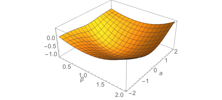
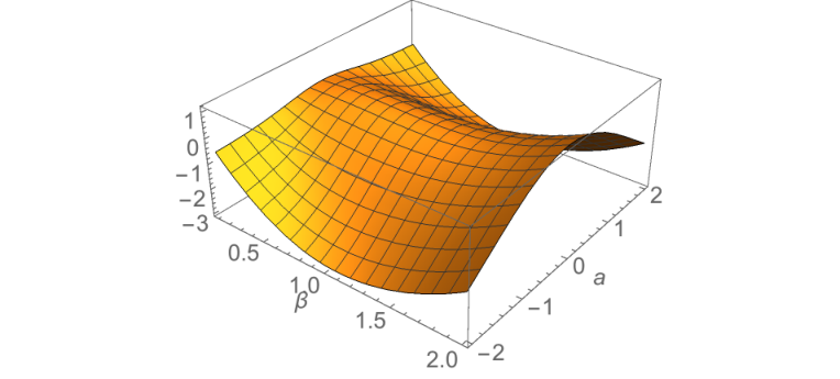
Using Derrick’s theorem we explored whether the solution was a maximum or minimum of the energy landscape as a function of the stretching parameter $\beta$. Here we would like to do a similar analysis to study whether the energy increases or decreases as we let $x\rightarrow x+a$ where $a$ is a small translation. Again we will posit that there is a translational instability if the energy $H[a]$ decreases as $a$ departs from zero. Let us again consider NLSE plus real potential

$${\rm i}\psi_{t}+\psi_{xx}+g|\psi|^{2\kappa}\psi-V(x)\psi=0\>,$$

(39)

where $V(x)=-\lambda\tilde{b}^{2}\sech^{2}(x)$. We want to see how the energy of the system changes under the translation $x\rightarrow x+a$ with the normalization fixed by the requirement that the mass $M$ is preserved. Clearly choosing

$$\psi_{a}=\psi(x+a)$$

(40)

preserves the mass for the wave function of the exact solution whose $x$ dependence is displayed by letting

$$\psi(x)=A(b,\gamma)\sech^{\gamma}(x)e^{i\gamma^{2}t}$$

(41)

It is also clear that both $H_{1}$ and $H_{2}$ remain unchanged under $x\rightarrow x+a$. Only $H_{3}$ is not translationally invariant. We define

	$\displaystyle H_{3}(a,\gamma)$	$\displaystyle=\!\int\!\differential{x}V(x)|\psi_{a}|^{2}$		(42)
		$\displaystyle=\lambda\tilde{b}^{2}A_{0}^{2}\int dx\sech^{2}(x)\sech^{2\gamma}(x+a)$
		$\displaystyle=\lambda\tilde{b}^{2}A_{0}^{2}\int dy\sech^{2}(y-a)\sech^{2\gamma}(y)\>.$

We need to ensure that as a function of $a$ the energy is stationary. Since both $H_{1}$ and $H_{2}$ are independent of $a$ we only need to consider:

$$\partialderivative{H_3(a,\lambda)}{a}\Big|_{a=0}$$

(43)

at $\beta=1$ and then calculate the second derivative at $\beta=1$. Clearly

		$\displaystyle\partialderivative{H_{\beta}}{a}=\partialderivative{H_{3 a}}(a)=$		(44)
		$\displaystyle-2\lambda\tilde{b}^{2}A_{0}^{2}\!\int\!\differential{y}\sech^{2}(y-a)\tanh(y-a)\sech^{2\gamma}(y)\>,$

which is indeed zero when evaluated at $a=0$, being an odd function of $y$. The second derivative gives

		$\displaystyle\partialderivative[2]{H_{a}}(a)=\partialderivative[2]{H_{3 a}}{a}=$		(45)
		$\displaystyle 2\lambda\tilde{b}^{2}A_{0}^{2}\!\int\!\differential{y}\sech^{2\gamma}(y)\,[\,3\sech^{4}(y-a)-2\sech^{2}(y-a)\,].$

Evaluating this at $a=0$ we find:

$$\partialderivative[2]{H_{a}}{a}\Big|_{a=0}=2\lambda\tilde{b}^{2}A_{0}^{2}\frac{\sqrt{\pi}\,\gamma\,\Gamma[\,\gamma+1\,]}{\Gamma[\,\gamma+5/2\,]}\>.$$

(46)

Thus we indeed find that the solitary wave has translational instability if $\lambda<0$, i.e. for the repulsive potential, while it is stable in case $\lambda>0$, i.e. attractive potential. Note that the answer does not depend on the sign of $g$. We show in Fig. 2 the three-dimensional landscape for $H(\beta,a)$ for a stretching and displacement shift, $x\rightarrow\beta x+a$. One can see stability for an attractive potential (case I) but a saddle point for a repulsive potential (case II).

The traditional way to study stability under small perturbations is to perform a linear stability analysis which we now present. The results obtained agree with the simpler analysis using Derrick’s theorem and looking at the effects of translation on the energy landscape. Starting with the NLSE equation in an external potential:

$$\{\,{\rm i}\,\partial_{t}+\partial_{x}^{2}+g\,\absolutevalue{\psi(x,t)}^{2\kappa}-V(x)\,\}\,\psi(x,t)=0\>,$$

(47)

which has solitary wave solutions $\psi(x,t)=\phi_{\omega}(x)\,{\rm e}^{-{\rm i}\omega t}$, with $\phi_{\omega}(x)\in\mathbb{R}$. Here $\phi_{\omega}(x)$ satisfies

$$\{\,\omega+\partial_{x}^{2}+g\,\absolutevalue{\phi_{\omega}(x)}^{2\kappa}-V(x)\,\}\,\phi_{\omega}(x)=0\>.$$

(48)

For $\omega=-\gamma^{2}$, one has the explicit expression:

$$\phi_{-\gamma^{2}}(x)=A_{0}(\tilde{b},\gamma)\,\sech^{\gamma}(x)\>.$$

(49)

We consider perturbations in the form $\psi(x,t)=(\phi_{\omega}(x)+r(x,t)){\rm e}^{-{\rm i}\omega t}$ with $r(x,t)\in\mathbb{C}$ and linearize the equation (47) with respect to $r(x,t)$. The linearized equation is of the form

		$\displaystyle\{\,\omega+{\rm i}\partial_{t}+\partial_{x}^{2}+V(x)+g\absolutevalue{\phi_{\omega}(x)}^{2\kappa}\,\}\,r(x,t)$		(50)
		$\displaystyle\qquad+2\kappa\,g\,\absolutevalue{\phi_{\omega}(x)}^{2\kappa}\Re{r(x,t)}=0\>.$

Because of the term $\Re{r(x,t)}$, Eq. (50) is not a $\mathbb{C}$-linear operator. For computational convenience we separate the real and imaginary parts of $r(x,t)$ and define

$$R(x,t)=\begin{pmatrix}p(x,t)\\ q(x,t)\end{pmatrix}=\begin{pmatrix}\Re{r(x,t)}\\ \Im{r(x,t)}\end{pmatrix}\>.$$

(51)

The equation (50) can then be written as

$$\partial_{t}R=\mathbf{JL}\,R$$

(52)

where

$$\mathbf{J}=\begin{pmatrix}0&1\\ -1&0\end{pmatrix},\quad\mathbf{L}=\begin{pmatrix}L_{+}&0\\ 0&L_{-}\end{pmatrix}$$

(53)

with self-adjoint operators

	$\displaystyle L_{-}(\omega)$	$\displaystyle=-\partial_{x}^{2}+V(x)-\omega-g\absolutevalue{\phi_{\omega}(x)}^{2\kappa}\>,$		(54a)
	$\displaystyle L_{+}(\omega)$	$\displaystyle=L_{-}(\omega)-2\kappa g\absolutevalue{\phi_{\omega}(x)}^{2\kappa}\>.$		(54b)

From (48) and its derivative with respect to $\omega$, we find

$$L_{-}(\omega)\,\phi_{\omega}(x)=0,\quad L_{+}(\omega)\,\partial_{\omega}\phi_{\omega}(x)=\phi_{\omega}(x)\>.$$

(55)

To explore the linear stability we consider eigenvalues for the operator $\mathbf{JL}$. Since

$$\mathbf{(JL)}^{2}=\begin{pmatrix}-L_{-}(\omega)L_{+}(\omega)&0\\ 0&-L_{+}(\omega)L_{-}(\omega)\end{pmatrix}$$

(56)

and the nonzero eigenvalues of $(-L_{-}L_{+})$ and $(-L_{+}L_{-})$ coincide, we can consider eigenvalues of the operator $(-L_{-}L_{+})$ instead. If $(-L_{-}L_{+})$ has eigenvalues with positive real part, so does $\mathbf{JL}$ and the solitary wave solutions are linearly unstable; otherwise, $\mathbf{JL}$ only has purely imaginary eigenvalues and the solitary wave solutions are spectrally stable.

For case (II) $g=+1$, $\lambda=-1$ we have $\omega=-\gamma^{2}$. The amplitude $\phi_{\omega}(x)$ is in $L^{2}$ and $L_{-}(\omega)\phi_{\omega}=0$, so $\phi_{\omega}$ is an eigenfunction of $L_{-}(\omega)$, corresponding to zero eigenvalue. Since $\phi_{\omega}$ is positive, $L_{-}(\omega)$ is nonnegative and the kernel $\ker(L_{-}({\omega}))$ is span$\{\phi_{\omega}\}$ by Proposition 2.8 in [35]. Due to (55) $\partial_{\omega}\phi_{\omega}$ is an eigenfunction of $L_{-}L_{+}$, corresponding to zero eigenvalue. We will show that the smallest eigenvalue of $L_{-}L_{+}$ is negative. According to Ref. [36] the smallest eigenvalue of $L_{-}L_{+}$ is given by,

$$\min\sigma_{d}(L_{-}L_{+})=\min\Big\{\,\frac{\expectationvalue{ u, L_ + u }}{\expectationvalue{u, L_-^{-1} u }},u\in\ker(L_{-})^{\perp}\Big\}\>.$$

(57)

$L_{-}$ is positive definite in $\ker(L_{-})^{\perp}$, so the sign of smallest eigenvalue is decided by that of $\langle u,L_{+}u\rangle$. Since $\phi_{\omega}(x)$ is an even function, $\partial_{x}\phi_{\omega}(x)$ is an odd function in $\ker(L_{-})^{\perp}$. Due to the identity

$$\partial_{x}(L_{-}\phi_{\omega}(x))=L_{+}\partial_{x}\phi_{\omega}(x)+V^{\prime}(x)\phi_{\omega}(x)=0\>,$$

(58)

one has that $L_{+}\partial_{x}\phi_{\omega}(x)=-V^{\prime}(x)\phi_{\omega}(x)$. Hence we have

		$\displaystyle\expectationvalue{ \partial_{x}\phi_{\omega}, L_ + \partial_{x}\phi_{\omega} }=\expectationvalue{ \partial_{x}\phi_{\omega}, -V'(x)\phi_{\omega} }$		(59)
		$\displaystyle\qquad\qquad=\frac{1}{2}\,\expectationvalue{ \phi_{\omega}, V''(x) \phi_{\omega} }\approx-0.455<0\>.$

It follows that $\expectationvalue{u, L_+u}$ can be negative and thus $(-L_{-}L_{+})$ has at least one positive eigenvalue. We conclude that the solitary wave solutions are linearly unstable.

For case (III) $g=-1$, $\lambda=+1$ we know that $L_{-}$ is nonnegative as in case (II). Since $-2\kappa g\absolutevalue{\phi_{\omega}(x)}^{2\kappa}$ is positive, $L_{+}$ is positive as well. It implies that $-L_{-}L_{+}$ has only negative eigenvalues and the solitary wave solutions are spectrally stable.

In order to study the dynamics in a collective coordinate approximation as well as determine the frequency of small oscillations (or the intitial growth of instabilities) we will now consider a four-parameter trial wave function of the form:

$$\tilde{\psi}(x,t)=A(t)\,\sech^{\gamma}[\,\beta(t)\,y(x,t)\,]\,{\rm e}^{{\rm i}\,\tilde{\phi}(x,t)}\>,$$

(60)

where

$$\tilde{\phi}(x,t)=-\theta(t)+p(t)\,y(x,t)+\Lambda(t)\,y^{2}(x,t)\>.$$

(61)

Here we have put $y(x,t)=x-q(t)$. The parameter $\Lambda$ is related to the canonical conjugate variable to the average value of $y^{2}$. It arises naturally in the Hartree-Fock approximation to the dynamics of the Schrödinger equation [37].

It will be useful to define a reciprocal width parameter $G(t)=1/\beta(t)$ and use this parameter as a generalized coordinate. Conservation of probability gives the “mass” equation,

$$M=\!\int\!\differential{x}\rho(x,t)=G(t)\,A^{2}(t)\,c_{1}[\gamma],$$

(62)

where $c_{1}[\gamma]$ is given in Eq. (10). In order to maintain probability conservation, we want to keep $M$ constant. That is, we put

$$A^{2}(t)=\frac{M}{G(t)\,c_{1}[\gamma]}$$

(63)

so $A(t)$ and $G(t)$ are not independent variables. The phase $\theta(t)$ does not enter into the Hamiltonian, and we will ignore it in what follows. The trial wave function we will assume is:

$$\tilde{\psi}(x,t)=\sqrt{\frac{M}{G\,c_{1}[\gamma]}}\,\sech^{\gamma}(y/G)\,{\rm e}^{{\rm i}\,[\,p\,y+\Lambda\,y^{2}\,]}\>.$$

(64)

The four variational parameters are labeled by

$$Q^{i}(t)=\quantity{\, q(t), p(t), G(t), \Lambda(t) \,}\>.$$

(65)

Taking the appropriate derivatives we find that

$$L_{0}=\frac{{\rm i}}{2}\,\!\int\!\differential{x}[\,\tilde{\psi}^{\ast}\,\tilde{\psi}_{t}-\tilde{\psi}^{\ast}_{t}\,\tilde{\psi}\,]=\pi_{i}(Q)\,\dot{Q}^{i}\>,$$

(66)

where

	$\displaystyle\pi_{q}$	$\displaystyle=p\,M\>,$		(67a)
	$\displaystyle\pi_{p}$	$\displaystyle=0$		(67b)
	$\displaystyle\pi_{\beta}$	$\displaystyle=0\>,$		(67c)
	$\displaystyle\pi_{\Lambda}$	$\displaystyle=-MG^{2}\,c_{2}[\gamma]/c_{1}[\gamma]\>,$		(67d)

with $c_{2}[\gamma]$ given in Eq. (35). The only non-zero derivatives of the $\pi_{i}$ are

$$\partial_{p}\pi_{q}=M,\quad\partial_{G}\pi_{\Lambda}=-2MG\,c_{2}[\gamma]/c_{1}[\gamma]\>,$$

(68)

so the symplectic tensor is

$$f_{ij}(Q)=M\begin{pmatrix}0&-1&0&0\\ 1&0&0&0\\ 0&0&0&-C\\ 0&0&C&0\end{pmatrix},\quad C=2\,G\,\frac{c_{2}[\gamma]}{c_{1}[\gamma]}\>,$$

(69)

and the inverse is

$$f^{ij}(Q)=\frac{1}{MC}\begin{pmatrix}0&C&0&0\\ -C&0&0&0\\ 0&0&0&1\\ 0&0&-1&\\ \end{pmatrix}\>.$$

(70)

We also find that for the four-parameter trial wave function

$$H=H_{1}+H_{2}+H_{3}\>,$$

(71)

where

	$\displaystyle H_{1}$	$\displaystyle=\!\int\!\differential{x}|\tilde{\psi}_{x}|^{2}$		(72a)
		$\displaystyle=M\,p^{2}+\frac{M}{G^{2}}\,\frac{\gamma}{2}\,\frac{c_{1}[\gamma+1]}{c_{1}[\gamma]}+4\,MG^{2}\Lambda^{2}\,\frac{c_{2}[\gamma]}{c_{1}[\gamma]}\>,$
	$\displaystyle H_{2}$	$\displaystyle=-\frac{g}{\kappa+1}\!\int\!\differential{x}|\tilde{\psi}|^{2\kappa+2}$		(72b)
		$\displaystyle=-\frac{gM\,\gamma}{\gamma+1}\,\quantity(\, \frac{M}{G \,c_1[\gamma]} \,)^{1/\gamma}\,\frac{c_{1}[\gamma+1]}{c_{1}[\gamma]}$
	$\displaystyle H_{3}$	$\displaystyle=\!\int\!\differential{x}V(x)\,|\tilde{\psi}|^{2}=-\lambda\,\tilde{b}^{2}\,M\,\frac{f_{1}[G,q,\gamma]}{c_{1}[\gamma]}\>,$		(72c)

with

$$f_{1}[G,q,\gamma]=\!\int\!\differential{z}\sech^{2\gamma}(z)\sech^{2}(Gz+q).$$

(73)

The Hamiltonian then becomes

		$\displaystyle\frac{H(Q)}{M}=p^{2}+\frac{\gamma}{2\,G^{2}}\,\frac{c_{1}[\gamma+1]}{c_{1}[\gamma]}+4\,G^{2}\Lambda^{2}\,\frac{c_{2}[\gamma]}{c_{1}[\gamma]}$		(74)
		$\displaystyle\quad-\frac{g\,\gamma}{\gamma+1}\,\quantity(\, \frac{M}{G \,c_1[\gamma]} \,)^{1/\gamma}\,\frac{c_{1}[\gamma+1]}{c_{1}[\gamma]}-\lambda\,\tilde{b}^{2}\,\frac{f_{1}[G,q,\gamma]}{c_{1}[\gamma]}\>.$

Derivatives of the Hamiltonian, $v_{i}=\partial_{i}H(Q)$, are given by

	$\displaystyle\frac{v_{q}}{M}$	$\displaystyle=2\lambda\,\tilde{b}^{2}\frac{f_{2}[G,q,\gamma]}{c_{1}[\gamma]}\>,$		(75a)
	$\displaystyle\frac{v_{p}}{M}$	$\displaystyle=2\,p\>,$		(75b)
	$\displaystyle\frac{v_{G}}{M}$	$\displaystyle=-\frac{\gamma}{G^{3}}\,\frac{c_{1}[\gamma+1]}{c_{1}[\gamma]}+8\,G\Lambda^{2}\,\frac{c_{2}[\gamma]}{c_{1}[\gamma]}$		(75c)
		$\displaystyle\!\!\!\!\!\!\!\!+\frac{g}{\gamma+1}\,\frac{1}{G}\,\quantity(\, \frac{M}{G \,c_1[\gamma]} \,)^{1/\gamma}\,\frac{c_{1}[\gamma+1]}{c_{1}[\gamma]}+2\,\lambda\,\tilde{b}^{2}\,\frac{f_{3}[G,q,\gamma]}{c_{1}[\gamma]}\>,$
	$\displaystyle\frac{v_{\Lambda}}{M}$	$\displaystyle=8\,G^{2}\Lambda\,\frac{c_{2}[\gamma]}{c_{1}[\gamma]}\>.$		(75d)

where

		$\displaystyle f_{2}[G,q,\gamma]=-\frac{1}{2}\,\partial_{q}f_{1}[G,q,\gamma]$		(76a)
		$\displaystyle\quad=\!\int\!\differential{z}\sech^{2\gamma}(z)\sech^{2}(Gz+q)\tanh( G z + q )\>,$
		$\displaystyle f_{3}[G,q,\gamma]=-\frac{1}{2}\,\partial_{G}f_{1}[G,q,\gamma]$		(76b)
		$\displaystyle\quad=\!\int\!\differential{z}z\,\sech^{2\gamma}(z)\sech^{2}(Gz+q)\tanh( G z + q)\>.$

From Eq. (21) and using (70), we find

	$\displaystyle\dot{q}$	$\displaystyle=\frac{v_{p}}{M}=2\,p\>,$		(77a)
	$\displaystyle\dot{p}$	$\displaystyle=-\frac{v_{q}}{M}=-2\lambda\,\tilde{b}^{2}\,\frac{f_{2}[G,q,\gamma]}{c_{1}[\gamma]}\>,$		(77b)
	$\displaystyle\dot{G}$	$\displaystyle=\frac{v_{\Lambda}}{MC}=4\,G\,\Lambda\>,$		(77c)
	$\displaystyle\dot{\Lambda}$	$\displaystyle=-\frac{v_{G}}{MC}=-\frac{1}{2G}\,\frac{c_{1}[\gamma]}{c_{2}[\gamma]}\,\frac{v_{G}}{M}$
		$\displaystyle=-4\Lambda^{2}+\frac{\gamma}{2\,G^{4}}\,\frac{c_{1}[\gamma+1]}{c_{2}[\gamma]}$		(77d)
		$\displaystyle\quad-\frac{g}{2(\gamma+1)}\,\frac{1}{G^{2}}\,\quantity(\, \frac{M}{G \,c_1[\gamma]} \,)^{1/\gamma}\,\frac{c_{1}[\gamma+1]}{c_{2}[\gamma]}$
		$\displaystyle\quad-\frac{\lambda\,\tilde{b}^{2}}{G}\,\frac{f_{3}[G,q,\gamma]}{c_{2}[\gamma]}\>.$

Recall that from (63),

$$g\,\quantity(\, \frac{M}{G(t) \, c_1[\gamma]} \,)^{1/\gamma}=g\,A^{2/\gamma}(t)\>,$$

(78)

and since $G(0)=1$ at $t=0$, we can use Eq. (7) to find:

$$g\,\quantity(\, \frac{M}{c_1[\gamma]} \,)^{1/\gamma}=g\,A^{2/\gamma}_{0}=\gamma(\gamma+1)-\lambda\tilde{b}^{2}\>.$$

(79)

So the dynamic equations (77) reduce to:

	$\displaystyle\dot{q}$	$\displaystyle=2\,p\>,$		(80a)
	$\displaystyle\dot{p}$	$\displaystyle=-2\lambda\,\tilde{b}^{2}\,\frac{f_{2}[G,q,\gamma]}{c_{1}[\gamma]}\>,$		(80b)
	$\displaystyle\dot{G}$	$\displaystyle=4\,G\,\Lambda\>,$		(80c)
	$\displaystyle\dot{\Lambda}$	$\displaystyle=-4\,\Lambda^{2}+\frac{1}{G^{4}}\,\frac{\gamma^{2}}{2\gamma+1}\,\frac{c_{1}[\gamma]}{c_{2}[\gamma]}$		(80d)
		$\displaystyle\quad-\frac{\gamma\,[\,\gamma(\gamma+1)-\lambda\,\tilde{b}^{2}\,]}{(2\gamma+1)(\gamma+1)}\,\frac{1}{G^{2+1/\gamma}}\,\frac{c_{1}[\gamma]}{c_{2}[\gamma]}$
		$\displaystyle\quad-\frac{\lambda\,\tilde{b}^{2}}{G}\,\frac{f_{3}[G,q,\gamma]}{c_{2}[\gamma]}\>,$

and are independent of $g$. We need to remember that for case III when $g=-1$ and $\lambda=+1$ there is no solution unless $\tilde{b}^{2}>\gamma(\gamma+1)$.

References

- [1] P. G. Kevrekidis, J. Cuevas-Maraver, A. Saxena, F. Cooper, and A. Khare, “Interplay between parity-time symmetry, supersymmetry, and nonlinearity: An analytically tractable case example,” Phys. Rev. E 92, 042901 (2015).
- [2] C. M. Bender, “Making sense of non-Hermitian Hamiltonians,” Rep. Prog. Phys. 70, 947 (2007).
- [3] Hendrik Geyer, Dieter Heiss, and Miloslav Znojil, “The physics of non-hermitian operators,” Journal of Physics A: Mathematical and General 39 (2006).
- [4] A. Fring, H. Jones, and M. Znojil, “6th international workshop on pseudo-hermitian hamiltonians in quantum physics,” Journal of Physics A: Mathematical and Theoretical 41, 240301 (2008).
- [5] C. M. Bender, A. Fring, U. Günther, and H. Jones, “Quantum physics with non-hermitian operators,” Journal of Physics A: Mathematical and Theoretical 45, 440301 (2012).
- [6] K. G. Makris, R. El-Ganainy, D. N. Christodoulides, and Z. H. Musslimani, “-Symmetric Periodic Optical Potentials,” International Journal of Theoretical Physics 50, 1019–1041 (2011).
- [7] A Ruschhaupt, F Delgado, and J G Muga, “Physical realization of -symmetric potential scattering in a planar slab waveguide,” Journal of Physics A: Mathematical and General 38, L171 (2005).
- [8] K. G. Makris, R. El-Ganainy, D. N. Christodoulides, and Z. H. Musslimani, “Beam dynamics in symmetric optical lattices,” Phys. Rev. Lett. 100, 103904 (2008).
- [9] Shachar Klaiman, Uwe Günther, and Nimrod Moiseyev, “Visualization of branch points in -symmetric waveguides,” Phys. Rev. Lett. 101, 080402 (2008).
- [10] S. Longhi, “Bloch oscillations in complex crystals with symmetry,” Phys. Rev. Lett. 103, 123601 (2009a).
- [11] S. Longhi, “Dynamic localization and transport in complex crystals,” Phys. Rev. B 80, 235102 (2009b).
- [12] S. Longhi, “Spectral singularities and bragg scattering in complex crystals,” Phys. Rev. A 81, 022102 (2010).
- [13] Christian E. Ruter, Konstantinos G. Makris, Ramy El-Ganainy, Demetrios N. Christodoulides, Mordechai Segev, and Detlef Kip, “Observation of parity-time symmetry in optics,” Nat Phys 6, 192–195 (2010).
- [14] A. Guo, G. J. Salamo, D. Duchesne, R. Morandotti, M. Volatier-Ravat, V. Aimez, G. A. Siviloglou, and D. N. Christodoulides, “Observation of -symmetry breaking in complex optical potentials,” Phys. Rev. Lett. 103, 093902 (2009).
- [15] Alois Regensburger, Christoph Bersch, Mohammad-Ali Miri, Georgy Onishchukov, Demetrios N. Christodoulides, and Ulf Peschel, “Parity-time synthetic photonic lattices,” Nature 488, 167–171 (2012).
- [16] Joseph Schindler, Ang Li, Mei C. Zheng, F. M. Ellis, and Tsampikos Kottos, “Experimental study of active lrc circuits with symmetries,” Phys. Rev. A 84, 040101 (2011).
- [17] J Schindler, Z Lin, J M Lee, H Ramezani, F M Ellis, and T Kottos, “-symmetric electronics,” Journal of Physics A: Mathematical and Theoretical 45, 444029 (2012).
- [18] C. M. Bender, B. K. Berntson, D. Parker, and E. Samuel, “Observation of phase transition in a simple mechanical system,” Am. J. Phys. 81, 173 (2013).
- [19] Bo Peng, Sahin Kaya Ozdemir, Fuchuan Lei, Faraz Monifi, Mariagiovanna Gianfreda, Gui Lu Long, Shanhui Fan, Franco Nori, Carl M. Bender, and Lan Yang, “Parity-time-symmetric whispering-gallery microcavities,” Nat Phys 10, 394–398 (2014).
- [20] Mohammad-Ali Miri, Matthias Heinrich, Ramy El-Ganainy, and Demetrios N. Christodoulides, “Supersymmetric optical structures,” Phys. Rev. Lett. 110, 233902 (2013).
- [21] Matthias Heinrich, Mohammad-Ali Miri, Simon Stützer, Ramy El-Ganainy, Stefan Nolte, Alexander Szameit, and Demetrios N. Christodoulides, “Supersymmetric mode converters,” Nature Communications 5, 3698 EP – (2014).
- [22] L É Gendenshteĭn and I V Krive, “Supersymmetry in quantum mechanics,” Soviet Physics Uspekhi 28, 645 (1985).
- [23] F. Cooper, A. Khare, and U. Sukhatme, “Supersymmetry and quantum mechanics,” Phys. Rept. 251, 267–385 (1995).
- [24] B Bagchi and R Roychoudhury, “A new -symmetric complex Hamiltonian with a real spectrum,” Journal of Physics A: Mathematical and General 33, L1 (2000).
- [25] B. Bagchi, S. Mallik, and C. Quesne, “Generating complex potentials with real eigenvalues in supersymmetric quantum mechanics,” International Journal of Modern Physics A 16, 2859–2872 (2001).
- [26] B. Bagchi and C. Quesne, “sl(2, C) as a complex Lie algebra and the associated non-Hermitian Hamiltonians with real eigenvalues,” Physics Letters A 273, 285 – 292 (2000).
- [27] Zafar Ahmed, “Real and complex discrete eigenvalues in an exactly solvable one-dimensional complex pt-invariant potential,” Physics Letters A 282, 343 – 348 (2001).
- [28] Bikashkali Midya, “Supersymmetry-generated one-way-invisible -symmetric optical crystals,” Phys. Rev. A 89, 032116 (2014).
- [29] F. Cooper, A. Khare, and U. Sukhatme, Supersymmetry in Quantum Mechanics (World Scientific, Singapore; River Edge, N.J., 2001).
- [30] F. Cooper, A. Khare, A. Comech, B. Mihaila, J. F. Dawson, and A. Saxena, “Stability of exact solutions of the nonlionear Schrödinger equation in an external potential having supersymmetry and parity-time symmetry,” J. Phys. A: Math. Theor. 50, 015391 (2017).
- [31] G. Poschl and E. Teller, “Bemerkungen zur Quantenmechanik des anharmonischen Oszillators,” Z. Phys. 83, 143 (1933).
- [32] L. D. Landau and E. M. Lifshitz, Quantum Mechnics (Nauka, Moscow, 1989).
- [33] Arjendu K. Pattanayak and William C. Schieve, “Gaussian wave-packet dynamics: Semiquantal and semiclassical phase-space formalism,” Phys. Rev. E 50, 3601–3615 (1994).
- [34] G. H. Derrick, “Comments on nonlinear wave equations as models for elementary particles,” Journal of Mathematical Physics 5, 1252–1254 (1964), http://dx.doi.org/10.1063/1.1704233 .
- [35] Michael I. Weinstein, “Modulational stability of ground states of nonlinear schrödinger equations,” SIAM Journal on Mathematical Analysis 16, 472–491 (1985), http://dx.doi.org/10.1137/0516034 .
- [36] Sulem, Catherine and Sulem, Pierre-Louis, The nonlinear Schrödinger equation (Springer-Verlag, New York,, 1999) pp. xvi+350.
- [37] Fred Cooper, So-Young Pi, and Paul N. Stancioff, “Quantum dynamics in a time-dependent variational approximation,” Phys. Rev. D 34, 3831–3841 (1986).
- [38] W. H. Press, S. A. Teukolsky, W. T. Vetterling, and B. P. Flannery, Numerical Recipes in FORTRAN: The Art of Scientific Computing (Cambridge University Press, Cambridge, 1992).