Emerging Anisotropic Compact Stars in Gravity
Abstract
The possible emergence of compact stars has been investigated in the recently introduced modified Gauss-Bonnet gravity, where is the Gauss-Bonnet term and is the trace of the energy-momentum tensor [1]. Specifically, for this modified theory, the analytic solutions of Krori and Barua have been applied to anisotropic matter distribution. To determine the unknown constants appearing in Krori and Barua metric, the well-known three models of the compact stars namely 4U1820-30, Her X-I, and SAX J 1808.4-3658 have been used. The analysis of the physical behavior of the compact stars has been presented and the physical features like energy density and pressure, energy conditions, static equilibrium, stability, measure of anisotropy, and regularity of the compact stars, have been discussed.
Keywords: Gravity; Krori and Barua; Compact Stars.
PACS: 04.50.Kd; 04.20.Jb.
1 Introduction
In astrophysics, compact stars are generally being referred to as the white dwarfs, neutron stars including the hybrid and quark stars, and the black holes. White dwarfs and neutron stars originated due to the degeneracy pressure produced by the fundamental particles responsible for their formation. These stars are massive but volumetrically smaller objects, therefore with high densities. Usually, the exact nature of these compact stars is not known to us but they are believed to be the massive objects with a small radius. Excluding black holes, all the other types of compact stars are sometimes also known as the degenerate stars. In general relativity (GR), an analysis of configured equilibrium is essential due to the reason of compact stars having huge mass and density. This can be started in a general relativistic way by considering the Oppenheimer-Volkoff equations [2] for static spherically symmetric and hydrostatic equilibrium, given as
| (1) |
where , , and is the pressure, density, and mass of the star respectively, varying with radial coordinate . At ( the coordinate radius of the compact star), the total mass of compact star is determined as
| (2) |
The combination of these Oppenheimer-Volkoff equations with the equation of the sate (EoS) parameter when solved numerically results into different configurations of the compact stars with divisions of low and high densities [3, 4].
Schwarzschild [5] was the pioneer to present the spherically symmetric exact solutions of Einstein field equations. The outcome of the first solution was the exploration of space-time singularity which gave the idea of a black hole. The second non-trivial solution predicted the bounded compactness parameter i.e., in hydrostatic equilibrium for some static and spherically symmetric configured structure [6]. Investigation of compact stars (neutron stars, dark stars, quarks, gravastars, and black holes) has become now an interesting research pursuit in astrophysics despite being not the new one. Baade and Zwicky [7] studied the compact stellar objects and argued that supernova may turn into a smaller dense compact object which came true later on after the discovery of pulsars which are highly magnetized rotating neutrons [8, 9]. Ruderman [10] was the first one to explore that at the core of the compact stars, the nuclear density turns anisotropic. A number of investigations have been made to find the solutions of the field equations for spherically symmetric anisotropic configurations in different contexts [11]-[13]. The pressure of the fluid sphere splits into the tangential and radial pressures in anisotropic configurations. Different investigations reveal that the repulsive forces which construct the compact stars, are produced due to anisotropy. Kalam et al. [14] showed that the Krori and Barua metric [15] establishes the necessary conditions for the advocacy of an effective and stable approach in modelling the compact objects. From an integrated Tolman Oppenheimer-Volkoff (TOV) equation, the numerical simulations may be used to study the nature of the compact stars, using EoS parameter. Rahaman et al. [16, 17] used EoS Chaplygin gas to explore their physical characteristics by extending Krori and Barua models. Mak and Harko [18] used some standard models for spherically symmetric compact objects and explored exact solutions to find the physical parameters such as the energy density, radial and tangential pressures concluding that inside these stars, the parameters would remain positive and finite. Hossein et al. [19] studied the effects on anisotropic stars due to cosmological constant. Different physical properties such as mass, radius, and moment of inertia of neutron stars has been investigated and a comprehensive comparison has been established with GR and modified theories of gravity [20]. Some interesting investigations related to the structure of slow rotating neutron stars in gravity are accomplished by making use of two distinct hadronic and a strange matter EOS parameter [21]. For a comprehensive study, some fascinating results can be seen in [22]-[28].
As an alternative to the theory of GR, modified theories of gravity have played an important and pivotal role to reveal the hidden facts about the accelerating expansion of the universe. After being motivated by the original theory and using the complex lagrangian, modified theories of gravity like , , , and have been structured, where is the Ricci scalar, is the Gauss-Bonnet invariant term, and is the trace of energy momentum tensor. Some reviews and important discussions relating to different modified theories of gravity have been published by different researchers [29]-[42]. Das et al. [43] presented exact conformal solutions to describe the interior of a star in modified teleparallel gravity. In another work, Das et al. [44] explored several physical features of the model admitting conformal motion to describe the behavior of the compact stars using modified gravity. Sharif and Yousuf [45] investigated the stability conditions of collapsing object by considering the non-static and spherically symmetric space-time. The field equations of modified theory have been explored by implementing the perturbation approach [46]. The possible formation of compacts stars in modified theory of gravity by using the Krori and Barua metric for spherically symmetric anisotropic compact stars has been discussed [47, 48]. In a recently published paper [1], Sharif and Ikram presented a new modified theory of gravity and studied different energy conditions for Friedmann-Robertson-Walker (FRW) universe. They found that the massive test particles follow non-geodesic geometry lines due to the presence of an extra force. It is being expected that the theory may describe the late-time cosmic acceleration for some special choices of gravity models. We discussed the Noether symmetry approach to find the exact solutions of the field equations in theory of gravity [49]. In an other paper [50], we investigated the same modified Gauss-Bonnet gravity and used the Noether symmetry methodology to discuss some cosmologically important gravity models with anisotropic background reported for locally rotationally symmetric Bianchi type universe. We used two models to explore the exact solutions and found that the specific models of modified Gauss-Bonnet gravity may be used to reconstruct CDM cosmology without involving any cosmological constant. Thus it seems interesting to further explore the universe in this theory.
This paper is aimed to investigate the possible emergence of compact stars by constructing some viable stellar solutions in theory of gravity by choosing some specific models. The plan of our present study is as follows: In section 2, we give the fundamental formalism of gravity with anisotropic matter distribution. Section 3 is dedicated for the matching of the metric conditions. Some physical features of the present study in context of gravity model under consideration are given in Section 4. Lastly, we present some conclusive discussions.
2 Anisotropic Matter Distribution in Gravity
The general action for the modified is [1],
| (3) |
where the function consists of the Gauss-Bonnet term and the trace of the energy-momentum tensor , denotes the coupling constant, is for the determinant of the metric tensor, is the Ricci Scalar, and represents matter part of the Lagrangian. The Gauss-Bonnet term is defined as
| (4) |
where , and is the Reimann and Ricci tensors, respectively. The variation of Eq.(3) with respect to , and by setting , gives the following fourth order non-linear field equations
| (5) | |||||
where is the d’Alembertian operator, is the Einstein tensor, , , , and . Einstein equations can be reawakened by putting simply whereas field equations for are reproduced by replacing with in Eq.(5). The energy-momentum tensor denoted by can be defined as
| (6) |
Moreover, the metric dependent energy-momentum tensor may have the form
| (7) |
The usual anisotropic energy momentum tensor is given as
| (8) |
where and represents the tangential and radial pressures respectively while denotes the energy density. The four velocity is denoted by and the radial four vector by , satisfying
| (9) |
In this paper, we have chosen specifically the following model [49]
| (10) |
where is an analytic function comprised of Gauss-Bonnet term. In particular, we consider , a power law model of gravity proposed by Cognola et al. [51] with being an arbitrary real constant, and a positive real number. Here we take , with being some positive real number. Further, for the investigations on the compact stars we take the static, spherically symmetric space-time as
| (11) |
We parameterize metric (11) by taking and , given by Krori and Barua [15] and with the help of some physical assumptions, the arbitrary constants and will be calculated. The above set of functions are established to reach a singularity free structure for compact stars. Therefore, our main concern is to present these functions to the metric in a way to achieve the structure for the compact star under this extended model, free from the singularities in the neighbourhood of . To investigate the existence of the compact stars for the model , we have considered , , and . For these parametric values, the energy density and all the energy conditions remain positive for the model under investigation. It is worth mentioning here that one may opt for some other choices of these values for further analysis. The explicit expressions for the energy density , radial pressure , and the tangential pressure are obtained as
| (12) | |||||
| (13) | |||||
| (14) | |||||
where prime denotes the radial derivative.
3 Matching With Schwarzschild’s Exterior Metric
Whatever the geometry of the star is, either derived internally or externally, the intrinsic boundary metric remains the same. Thus, confirming that the components of the metric tensor irrespective of the coordinate system across the surface of the boundary will remain continuous. No doubt, in GR, the Schwarzschild solutions have been pioneer in guiding us to choose from the diverse possibilities of the matching conditions while investigating the stellar compact objects. Now when we come to the case of modified theories of gravity, modified TOV equations with zero pressure and energy density, the solution outside the star can differ from Schwarzschild’s solution. However, it is expected that the solutions of the modified TOV equations with energy density and pressure (may be non-zero) may accommodate Schwarzschild’s solution with some specific choice of gravity model. Perhaps this is the reason that Birkhoff’s theorem may not hold in modified gravity. The detailed investigation of the issue in the context of gravity can be an interesting task. Many authors have considered Schwarzschild solution for this purpose giving some interesting results [52]-[55]. Now to solve the field equations under the restricted boundary conditions at , the pressure , the interior metric (11) requires these matching conditions. This can be done by taking a smooth match at to Schwarzschild’s exterior metric, given by
| (15) |
yielding
| (16) |
where corresponds to exterior solution and to the interior solution. Now from the comparison of exterior and interior metrics, the constants , , and are obtained as
| (17) | |||||
| (18) | |||||
| (19) |
The approximated values of the mass and radius of the compact stars Her X-1, SAX J1808.4-3658 and 4U1820-30 are used to calculate the values of constants and [56, 57]. The result defines the compactness of the star and the expression determines the surface redshift . For the compact stars under consideration, the values of have been given below in table as follows.
| Compact Stars | ||||||
|---|---|---|---|---|---|---|
| Her X-1 | 0.88 | 7.7 | 0.168 | 0.006906276428 | 0.004267364618 | 0.23 |
| SAXJ1808.4-3658 | 1.435 | 7.07 | 0.299 | 0.01823156974 | 0.01488011569 | 0.57 |
| 4U1820-30 | 2.25 | 10.0 | 0.332 | 0.01090644119 | 0.009880952381 | 0.73 |
Now making use of Krori and Barua metric, Eqs. (12)-(14) take the form
| (20) | |||||
| (21) | |||||
| (22) | |||||
| where | (23) | ||||
| (24) | |||||
| (25) | |||||
Now we investigate the nature and some interesting features of the compact star, specifically for the assumed model of gravity.
4 Physical Aspects of Gravity Model
In this section, some interesting physical aspects of the compact stars such as the energy density and pressure evolutions, energy conditions, equilibrium conditions, stability and adiabatic index analysis, compactness, and redshift analysis shall be discussed.
4.1 Energy Density and Pressure Evolutions
 |
 |
 |
 |
 |
 |
 |
 |
 |
The plot of the energy density for the strange star candidate Her X-1 (Figure 1) shows that as , goes to maximum, and this in fact indicates the high compactness of the core of the star validating that our model under investigation is viable for the outer region of the core. The other two graphs in the same row provide us with similar sort of conclusions. Furthermore, from the other plots of the anisotropic radial pressure (Figure ), it is evident that the radius of the star for this model is km which further when used, gives us the density of g , a high value with a small radius of 10 km, showing that our model is compatible to the structure of ultra-compact star [10, 59]. A comparison of this with the already existing data, labels this compact star as quark/strange star [60]. All the three plots in Figure indicate that the tangential pressure remains positive and finite and show their decreasing behavior, which is required for the viability of the compact star model.
 |
 |
 |
 |
 |
 |
The variations of the radial derivatives of the density and radial pressure are shown in Figures (4) and (5) respectively. One can see the decreasing evolution of the first -derivatives i.e and . It may be noted here that at , these derivatives just disappear except of the radial pressure for the SAX J 1808.4-3658 candidate. The mathematical calculations for the second derivative test both for and tell us that and , indicating the maximum values of the density and radial pressure at the center. This further suggests the compact nature of the star.
4.2 Energy Conditions
 |
 |
 | |
 |
 |
 |
For the viability of the model, the energy bounds must be satisfied due to their significant importance in analysing the theoretical data. NEC (null energy conditions), WEC (weak energy conditions), SEC (strong energy conditions), and DEC (dominant energy conditions) have been given as
| NEC | ||||
| WEC | ||||
| SEC | ||||
| DEC |
The evolution of all these energy conditions have been well satisfied as represented graphically for the strange star candidate Her X-1 in Figure (6). Hence our solutions are physically viable.
4.3 Tolman-Oppenheimer-Volkoff (TOV) Equation
 |
In anisotropic case, the generalized TOV equation is given as
| (26) |
where
| (27) |
is the gravitational mass of a sphere of radius . Now putting Eq.(27) into Eq.(26), it follows
| (28) |
Eq.(28) gives the information about the stellar configuration equilibrium under the combined effect of different forces like the anisotropic force , the hydrostatic force , and the gravitational force . Their summation to zero eventually describes the equilibrium condition of the form
| (29) |
where
| (30) | |||||
From Figure (7), it can be noticed that under the mutual effect of the three forces , and , the static equilibrium might be achieved. It is mentioned here that at some point if then , which suggests that the equilibrium becomes independent of the anisotropic force .
4.4 Stability Analysis
 |
 |
 |
 |
 |
 |
For the stability, the radial and transversal sound speeds denoted by and respectively, should satisfy the bounds, and [61], where and . It can be seen from the Figures (8) and (9) that the evolution of the radial and transversal sound speeds for strange star candidate Her X-1 are within the bounds of stability as discussed, but in the case of SAX J 1808.4-3658, and 4U 1820-30 strange star candidates, the radial sound speeds evolution which is against the radial coordinate temporarily violates these stability conditions. However, for the same candidates the transversal sound speeds are satisfied. Within the matter distribution, the estimation of the potentially stable and unstable eras can be had from the differences of the propagations of the sound speeds which is the expression satisfying the inequality . This can be seen clearly from the plots of Figure (10). Thus, overall the stability may be attained for compact stars under gravity model, particularly for the strange star candidate Her X-1.
 |
 |
 |
4.5 Adiabatic Index Analysis
For the case of anisotropic fluid spherical star, as proposed in [62, 63], the stability depends on the adiabatic index , and for the radial and tangential cases, we respectively have
| (31) |
The stability of a Newtonian sphere should be satisfied if , and is the condition for the occurrence of neutral equilibrium [64]. Due to the presence of the effective pressure, the anisotropic relativistic sphere obeys more complicated stability condition given as
| (32) |
where , , and are the initial energy density, tangential pressure, and radial pressure in static equilibrium respectively satisfying Eq. (26). In our case, the adiabatic index has been calculated analytically for strange star candidate Her X-1 , giving us and , which shows the complete stability in radial case but some deviation in the tangential case.
4.6 Mass-Radius Relationship
 |
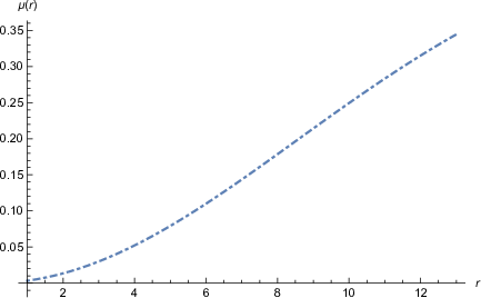
The mass of the compact star as a function of radius is given as
| (33) |
It can be seen clearly from the profile of the mass function given in Figure (11) that the mass of the star is directly proportional to the radius, and as , which depicts that the mass function is regular at the centre of the star. Moreover, for the spherically symmetric anisotropic perfect fluid case, the ratio of the mass to the radius, according to Buchdahl [6] should be bounded like . In our case, the situation is very good as we get and the condition is clearly satisfied.
4.7 Compactness and Redshift Analysis
 |
 |
Compactness of the star is expressed as
| (34) |
Therefore, the redshift is determined as
| (35) |
The graphical evolution of the surface redshift has been given in Figure (12). The value of the function for the case of the strange star candidate Her X-1 is calculated as which is within the desired bound of .
 |
 |
 |
 |
 |
 |
4.8 EoS Parameter and the Measurement of Anisotropy
Now for anisotropic case, the radial and transversal forms of EoS parameter can be written as
| (36) |
The evolution of these EoS parameters with the increasing radius have been shown in Figures (13 and 14) which clearly demonstrate that all the six plots satisfy the inequalities and . This further advocates the effectiveness of the considered model.
 |
 |
 |
The measurement of the anisotropy denoted by is given by
| (37) |
which gives the information about the anisotropic behavior of the model. The remains positive if , suggesting the anisotropy being drawn outward, and for the reverted situation, i.e., , the anisotropy turns negative which corresponds to being directed inward. For our situation, the variations of the anisotropic measurement with respect to the radial coordinate show the decreasing negative behavior for the strange star candidate Her X-1 and SAX J 1808.4-3658 suggesting that . For the 4U 1820-30 candidate, it remains positive for a fraction of the radius where some repulsive anisotropic force followed by massive matter distribution appears and very soon, it gets negative after .
5 Concluding Discussion
In this paper, we have put some useful discussions related to the emergence of compact stars in the newly introduced theory of gravity by considering the model . We have tested this model for the strange star candidates Her X-1, SAX J 1808.4-3658, and 4U 1820-30 for anisotropic case by using the Krori and Barua approach of metric function [15], that is, . The arbitrary constants , , and are calculated by smoothly matching the interior metric conditions with the Schwarzschild’s exterior metric conditions. This phenomenon makes us to understand the nature of the compact stars by expressing their masses and radii in terms of the arbitrary constants.
By using these constants in our investigation for the strange star candidates Her X-1, SAX J 1808.4-3658, and 4U 1820-30 the energy density, radial and tangential pressures have been plotted with respect to radial coordinate indicating that when approaches to zero, the density goes to its maximum for all the three strange star candidates. The same is the situation for the tangential pressure but different behavior in the case of the radial pressure for the 4U 1820-30 candidate. Mainly, this situation admits the theory that the core of compact stars under consideration, is intensely compact, particularly in case of the strange star candidate Her X-1. We have succeeded to determine the density of the emerging compact star after estimating the radius of the star from the evolution of the radial pressure. The evolution of EoS parameters with the increasing radius satisfies the inequalities and for the radial and tangential EoS parameters respectively, which favor the acceptance of the model under study. We have also shown through the graphical representation that all the energy conditions namely NEC, WEC, SEC, and DEC are satisfied for the proposed gravity model in the case of Her X-1 favoring the physical viability of the model.
The static equilibrium, to some extent, has been established by plotting the three forces , , and comprised in the TOV equation. The evolution of the radial and transversal sound speeds denoted by and respectively for strange star candidate Her X-1 are within the bounds of stability [61] , but in the case of SAX J 1808.4-3658, and 4U 1820-30 strange star candidates, the radial sound speed evolutions temporarily violate these stability conditions. However, for the same candidates the transversal sound speeds are satisfied. Within the matter distribution, the estimation of the strongly stable and unstable eras from the differences of the propagations of the sound speeds satisfies the inequality for all the candidates as shown in Figure . Thus, overall the stability is attained for compact star model, particularly for the strange star candidate Her X-1.
We have also investigated the dynamical stability by analytically calculating the adiabatic index of the model both for the radial and tangential pressures for strange star candidate Her X-1, giving us and , which shows the complete stability in radial case but a slight deviation in the tangential case. We have found the direct proportionality of the mass function to the radius, and as , suggesting that the mass function is regular at the center of the star. Moreover, for the spherically symmetric anisotropic fluid case, the ratio of the mass to the radius has been calculated as satisfying as proposed by Buchdahl [6]. The evolution of the compactness of the star for Her X-1 favors the model. The values of surface redshift function are within the bound of and for the case of the strange star candidate Her X-1, the redshift value is calculated as which satisfies the upper bound . This further indicates the stability of the model under study. Conclusively, for the case of the strange star candidate Her X-1, all the physical parameters have been more consistent to favor the gravity model under study as compared to the other two candidates SAX J 1808.4-3658 and 4U 1820-30. The overall consistency for the model may be improved by considering some more suitable choices of the physical parameters.
Acknowledgement
Many thanks to the anonymous reviewer
for valuable comments and suggestions to improve the paper.
This work was supported by National University
of Computer and Emerging Sciences (NUCES).
References
- [1] Sharif, M. and Ikram, A.: Eur. Phys. J. C 76 (2016) 640.
- [2] Oppenheimer, J.R. and Volkoff, G.: Phys. Rev. 55(1939) 374.
- [3] Negele, J.W. and Vautherin D.: Nucl. Phys. A 207 (1973) 298.
- [4] Akmal, A., Pandharipande, V. R. and Ravenhall, D.G.: Phys. Rev. C 58 (1998) 1804.
- [5] Schwarzschild, K.: Sitzer. Preuss. Akad. Wiss. 189 (1916) 424.
- [6] Buchdahl, H. A.: Phys. Rev. 116 (1959) 1027.
- [7] Baade, W. and Zwicky, F.: Phys. Rev. 46 (1934) 76.
- [8] Longair, M.S.: High Energy Astrophysics (Cambridge Univeristy Press, 1994).
- [9] Ghosh, P.: Rotation and Accretion Powered Pulsars(World Scientific, 2007).
- [10] Ruderman, R.: Annu. Rev. Astron. Astrophys. 10 (1972) 427.
- [11] Maurya, S.K. and Gupta, Y.K.: Astrophys. Space Sci. 344 (2013) 243.
- [12] Maurya, S.K. and Gupta, Y.K.: Phys. Scr. 86 (2012) 025009.
- [13] Maharaj, S.D., Sunzu, J.M., and Ray, S.: Eur. Phys. J. Plus 129 (2014) 3.
- [14] Kalam, M. et al.: Eur. Phys. J.C 72 (2012) 2248.
- [15] Krori, K.D. and Barua, J.: J. Phys. A: Math. Gen. 8 (1975) 508.
- [16] Rahaman, F. et al.: Gen. Relativ. Grav. 44 (2012) 107.
- [17] Rahaman, F. et al.: Eur. Phys. J. C 72 (2012) 2071.
- [18] Mak, M.K. and Harko, T.: Int. J. Mod. Phys. D 13 (2004) 149.
- [19] Hossein, S.K.M. et al.: Int. J. Mod. Phys. D 21 (2012) 1250088.
- [20] Yazadjiev, S. S., Doneva, D. D. and Kokkotas, K. D.: Phys. Rev. D 91 (2015) 084018.
- [21] Staykov, K. V., Doneva, D. D., Yazadjiev, S. S. and Kokkotas, K. D.: JCAP 10 (2014) 006
- [22] Nojiri, S. and Odintsov, S.D.: Phys. Rep. 505 (2011) 59.
- [23] Paliathanasis, A et al.: Phys. Rev. D 89 (2014) 104042.
- [24] Nojiri, S. and Odintsov, S.D.: Int. J. Geom. Meth. Mod. Phys. 4 (2007) 115.
- [25] Capozziello, S., Laurentis, M. D. and Odintsov, S.D.: Eur. Phys. J. C 72 (2012) 2068.
- [26] Capozziello, S., Laurentis, M. D. Odintsov, S.D. and Stabile, A.: Phys. Rev. D 83 (2011) 064004.
- [27] Astashenok, A. V., Capozziello, S., Laurentis, M. D. and Odintsov, S.D.: JCAP 1501 (2015) 001.
- [28] Capozziello, S., Laurentis, M. D., Farinelli, R., and Odintsov, S.D.: Phys. Rev. D 93 (2016) 023501.
- [29] Felice, A.D. and Tsujikaswa, S.: Living Rev. Rel. 13 (2010 ) 3.
- [30] Bamba, K., Capozziella, S., Nojiri, S. and Odintsov, S.D.: Astrophys. Space Sci. 342 (2012) 155.
- [31] Astashenok, A.V., Capozziello, S. and Odintsov, S.D.: Phys. Rev. D 89 (2014) 103509.
- [32] Astashenok, A.V., Capozziello, S. and Odintsov, S.D.: JCAP 01 (2015) 001.
- [33] Cognola, G., Elizalde, E., Nojiri, S., Odintsov, S.D. and Zerbini, S.: Phys. Rev. D 73 (2006) 084007.
- [34] Shamir, M.F.: Astrophys. Space Sci. 361 (2016) 147.
- [35] Shamir, M.F.: J. Exp. Theor. Phys. 123 (2016) 607.
- [36] Nojiri, S. and Odintsov, S.D.: Phys. Lett. B 631 (2005) 1.
- [37] Chiba, T.: J. Cosmol. Astropart. Phys. 03 (2005) 008.
- [38] Nojiri, S. and Odintsov, S.D. and Tretyakov, P.V.: Prog. Theor. Phys. Suppl. 172 (2008) 81.
- [39] Starobinsky, A. A.: J. Exp. Theor. Phy. 86 (2009) 157.
- [40] Harko, T., Lobo, F.S.N., Nojiri, S. and Odinttsov, S.D.: Phys. Rev. D 84 (2011) 024020.
- [41] Sharif, M. and Zubair, M.: J. Phys. Soc. Jpn. 82 (2013) 014002.
- [42] Sharif, M. and Zubair, M.: JCAP 03 (2012) 028.
- [43] Das, et al.: Astrophys. Space Sci. 358 (2015) 36.
- [44] Das, et al.: Eur. Phys. J. C 76 (2016) 654.
- [45] Sharif, M. and Yousuf, Z.: Astrophys. Space Sci. 354 (2014) 471.
- [46] Noureen, I. et al.: Eur. Phys. J. C 75 (2015) 323.
- [47] Zubair, M. and Noureen, I.: Eur. Phys. J. C 75 (2015) 265.
- [48] Zubair, M., Abbas, G. and Noureen, I.: Astrophys. Space Sci. 361 (2016) 8.
- [49] Shamir, M.F. and Ahmad, M.: Eur. Phys. J. C 77 (2017) 55.
- [50] Shamir, M.F. and Ahmad, M.: Mod. Phys. Lett. A 32 (2017) 1750086.
- [51] Cognola, G., Elizalde, E., Nojiri, S., Odintsov, S.D. and Zerbini, S.: Phys. Rev. D 75 (2007) 086002.
- [52] Cooney, A., DeDeo, S., and Psaltis, D.: Phys. Rev. D 82(2010) 064033.
- [53] Ganguly, A., Gannouji, R., Goswami, R., and Ray, S.: Phys. Rev. D 89(2014) 064019.
- [54] Momeni, D. and Myrzakulov, R.: Int. J. Geom. Methods Mod. Phys.12 (2015) 1550014.
- [55] Astashenok, A. V., Capozziello, S., Laurentis, M. D. and Odintsov, S.D.: JCAP 1312 (2013) 040.
- [56] Lattimer, J.M. and Steiner, A.W.: Astrophy. J. 784 (2014) 123.
- [57] Li, X.D. et al.: Phys. Rev. Lett. 83 (1999) 3776.
- [58] Glendenning, N.K. Compact Stars: Nuclear Physics, Particle Physics and General Relativity (Springer, NewYork, 1997).
- [59] Herjog, M. and Roepke, F.K.: Phys. Rev. D 84 (2011) 083002.
- [60] Bhar, P., Rahaman, S., Ray, S. and Chatterjee, V.: Eur. Phys. J. C 75 (2015) 190.
- [61] Herrera, L.: Phys. Lett. A 165 (1992)) 206.
- [62] Chandrasekhar, S.: Astrophys. J. 140 (1964) 417.
- [63] Heintzmann, H. and Hillebrandt, W.: Astron. Astrophys. 38 (1975) 51.
- [64] Bondi, H.: Proc. R. Soc. Lond. Series A Math. Phys. Sci. 281 (1964) 39.