跳到论文正文
W Papers独立论文阅读器 arXiv:1705.06837 论文正文 计算阅读时间 · 0%
引用这篇论文根据当前论文元数据生成,正式投稿前建议核对。


License: arXiv.org perpetual non-exclusive license
arXiv:1705.06837v3 [math.AP] 10 Mar 2020

Loss of Regularity of Solutions of the Lighthill Problem for Shock Diffraction for Potential Flow

Gui-Qiang Chen Address: Gui-Qiang G. Chen, Mathematical Institute, University of Oxford, Oxford, OX2 6GG, UK;  AMSS and UCAS, Chinese Academy of Sciences, Beijing 100190, China Email address: chengq@maths.ox.ac.uk , Mikhail Feldman Address: Mikhail Feldman, Department of Mathematics, University of Wisconsin, Madison, WI 53706-1388, USA Email address: feldman@math.wisc.edu , Jingchen Hu Address: Jingchen Hu, School of Mathematical Sciences, University of Science and Technology of China, Hefei, China Email address: jchu@mail.ustc.edu.cn and Wei Xiang Address: Wei Xiang, Department of Mathematics, City University of Hong Kong, Kowloon, Hong Kong, P. R. China Email address: weixiang@cityu.edu.hk
Date: August 24, 2026
Abstract.

We are concerned with the suitability of the main models of compressible fluid dynamics for the Lighthill problem for shock diffraction by a convex corned wedge, by studying the regularity of solutions of the problem, which can be formulated as a free boundary problem. In this paper, we prove that there is no regular solution that is subsonic up to the wedge corner for potential flow. This indicates that, if the solution is subsonic at the wedge corner, at least a characteristic discontinuity (vortex sheet or entropy wave) is expected to be generated, which is consistent with the experimental and computational results. Therefore, the potential flow equation is not suitable for the Lighthill problem so that the compressible Euler system must be considered. In order to achieve the non-existence result, a weak maximum principle for the solution is established, and several other mathematical techniques are developed. The methods and techniques developed here are also useful to the other problems with similar difficulties.

Key words and phrases:
Loss of regularity, free boundary problems, Lighthill problem, nonlinear equations of second order, mixed elliptic-hyperbolic type, degenerate elliptic equations, conservation laws, potential flow equation, shock diffraction, compressible flow
2010 Mathematics Subject Classification
Primary: 35M10, 35M12, 35B65, 35L65, 35L70, 35J70, 76H05, 35L67, 35R35; Secondary: 35L15, 35L20, 35J67, 76N10, 76L05

1. Introduction

We are concerned with the regularity of solutions of the Lighthill problem for shock diffraction by a two-dimensional convex cornered wedge, which is not only a longstanding open problem in fluid mechanics but also fundamental in the mathematical theory of multidimensional conservation laws, since the shock diffraction configurations are fundamental for the local structure of general entropy solutions. The Lighthill problem can be formulated as a free boundary problem.

The main objective of this paper is to address the fundamental issue: which of the main models of compressible fluid dynamics is suitable for the shock diffraction problem. There are two main models: the compressible Euler system and the potential flow equation. We prove that there is no regular solution of the shock diffraction problem in the framework of potential flow. In fact, our results show the limitation of the potential flow equation, since solutions of this equation have a high regularity, so that it is too rigid for the Lighthill problem. This shows that the Euler system may be more stable as it allows nonregular solutions.

The Euler equations for polytropic potential flow consist of

(1.1) ∂tρ+div𝐱​(ρ​∇𝐱Φ)=0\partial_{t}\rho+\mbox{div}_{\mathbf{x}}(\rho\nabla_{\mathbf{x}}\Phi)=0

with Bernoulli’s law:

(1.2) ∂tΦ+12​|∇𝐱Φ|2+i⁡(ρ)=B0,\partial_{t}\Phi+\frac{1}{2}|\nabla_{\mathbf{x}}\Phi|^{2}+i(\rho)=B_{0},

where 𝐱=(x1,x2)∈ℝ2\mathbf{x}=(x_{1},x_{2})\in\mathbb{R}^{2}, ρ\rho is the density, Φ\Phi is the velocity potential such that ∇𝐱Φ=:(u,v)=𝐯\nabla_{\mathbf{x}}\Phi=:(u,v)=\mathbf{v} is the flow velocity, and B0B_{0} is the Bernoulli constant determined by the incoming flow and/or boundary conditions. For a polytropic gas, by scaling,

c2​(ρ)=ργ−1,i⁡(ρ)=ργ−1−1γ−1,γ>1,c^{2}(\rho)=\rho^{\gamma-1},\quad i(\rho)=\frac{\rho^{\gamma-1}-1}{\gamma-1},\qquad\gamma>1,

where c⁡(ρ)c(\rho) is the sound speed. For the isothermal case, γ=1\gamma=1,

p⁡(ρ)=ρ,c2​(ρ)=1,i⁡(ρ)=l​n​ρp(\rho)=\rho,\qquad c^{2}(\rho)=1,\qquad i(\rho)=ln\rho

as the limiting case when γ→1\gamma\to 1. In this paper, we focus mainly on the case γ>1\gamma>1, since a similar argument works when γ=1\gamma=1.

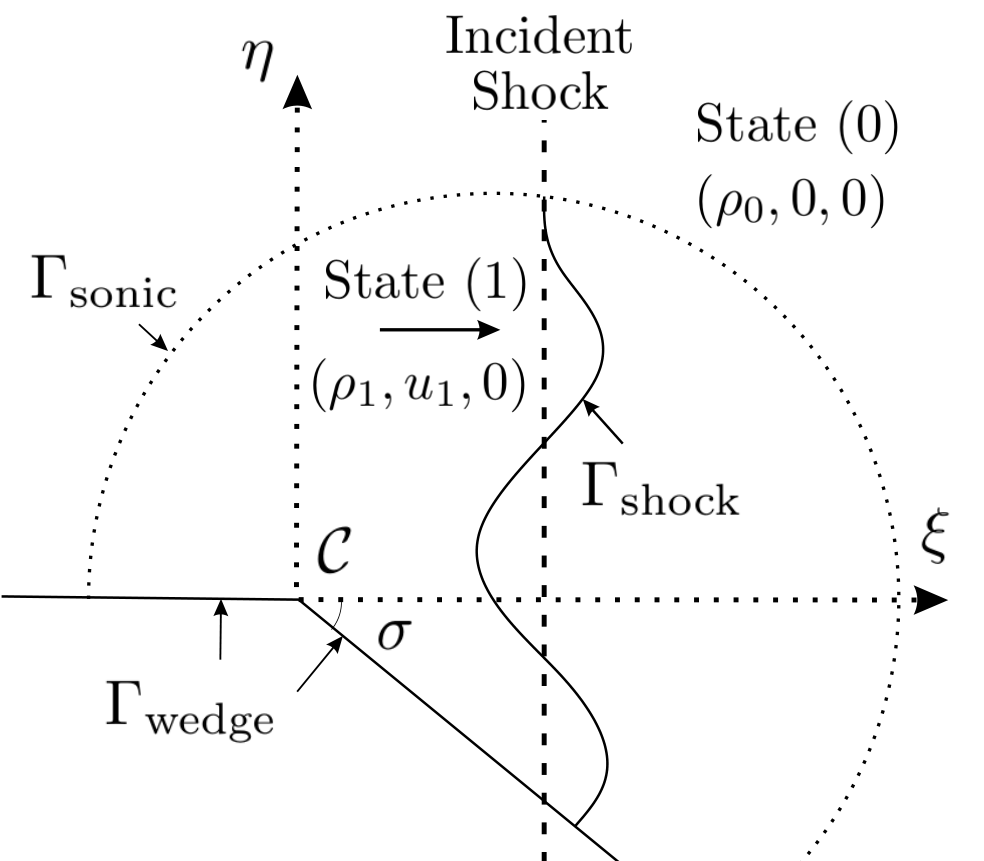
Figure 1.1. The Lighthill problem for shock diffraction

As shown in Fig. 1.1, we consider two piecewise constant Riemann data with the left state, State (1)(1): (ρ1,u1,0),u1>0(\rho_{1},u_{1},0),u_{1}>0, and the right state, State (0)(0): (ρ0,0,0)(\rho_{0},0,0), separated by a vertical shock S0S_{0} and above the wedge with the corner angle θw=π−σ\theta_{w}=\pi-\sigma, where σ∈(0,π)\sigma\in(0,\pi). As this incident shock passes through the wedge, the incident shock interacts with the sonic circle and becomes a transonic shock. On the other hand, physical observation and numerical analysis [26, 27] indicate that, when a shock is diffracted by a convex cornered wedge, at least a characteristic discontinuity (vortex sheet or entropy wave) should be generated. Mathematically, to confirm this phenomenon, one needs to show the nonexistence of regular solutions of the Lighthill problem. Therefore, we are interested in the question of whether any solution of the Lighthill problem, governed by the potential flow equation, is irregular at the wedge corner; that is, a regular solution, which is Lipschitz at the corner, does not exist, where the exact notion of regular solutions will be given in §2.3.

In this paper, we prove the nonexistence of regular solutions to this Riemann data when the initial left state (ρ1,u1,0)(\rho_{1},u_{1},0) is subsonic, i.e., u1<c1u_{1}<c_{1}. Then the pseudo-velocity (U,V)=(u1,0)(U,V)=(u_{1},0) at the origin is pseudosubsonic, and the degenerate boundary is the sonic circle centered at (u1,0)(u_{1},0) with radius c1c_{1}. One of the main ingredients in our analysis is to develop a weak maximum principle at the wedge corner for the velocity in a special direction by the integration method. It is well known that, if a regular solution is assumed to have a C1C^{1}-velocity at the wedge corner, then we can directly apply Hopf’s maximum principle to the directional derivative of the potential function to reach a contradiction. However, it does not apply directly to the solution that is not C2C^{2}-continuous. Therefore, it is the key point in §3 to develop the weak maximum principle without the C2C^{2}-continuity of the solution.

The mathematical study of the shock diffraction problem dates back to the 1950s by the work of Lighthill [21, 22] via asymptotic analysis, which is now called the Lighthill problem; also see Bargman [2], Fletcher, Weimer, and Bleakney [17], and Fletcher, Taub, and Bleakney [16] via experimental analysis, as well as Courant, and Friedrichs [12] and Whitham [28]. To date, all efforts for rigorous mathematical analysis of the Lighthill problem have focused on some simplified models. For one of these models, the nonlinear wave system, Kim [19] first studied this problem for the right wedge angle with an additional physical assumption that the transonic shock does not collide with the sonic circle of the right state. More recently, in Chen, Deng, and Xiang [7], this assumption was removed, and the existence and optimal regularity of shock diffraction configurations were established for all angles of the convex wedge via a different approach.

A closely related problem, shock reflection-diffraction by concave cornered wedges, has been systematically analyzed in Chen, and Feldman [8, 9], Bae, Chen, and Feldman [3] and Chen, Feldman, and Xiang [10, 11], where the existence and uniqueness of regular shock reflection-diffraction configurations has been established up to the detachment wedge angle. For the nonsymmetric case, the non-existence of regular solutions has been shown in Feldman, and Hu [15] when the wedge angle is sufficiently close to π\pi. The Prandtl-Meyer reflection for supersonic potential flow impinging onto a solid wedge has also been analyzed first in Elling, and Liu [13] and, most recently, in Bae, Chen, and Feldman [4, 5] for the general case. For other related references, we refer the reader to Serre [25] for Chaplygin gas, Canic, Keyfitz, and Kim [6] for the nonlinear wave system, and Zheng [29] for the pressure-gradient system. See also [14, 24] for steady flow passing through a wedge.

The organization of this paper is as follows: In §2, we formulate the Lighthill problem as a free boundary problem for a nonlinear equation of mixed elliptic-hyperbolic type, prove the important fact that the speed of incident shock is subsonic and the incident shock hits the sonic circle in the first quadrant, and then introduce the notion of regular solutions of the free boundary problem and state the main theorem. In §3, we prove the monotonicity property of regular solutions with respect to a special direction. This means that, if the regular solution exists, the speed along some direction cannot achieve the negative minimum anywhere in Ω¯\overline{\Omega}. Then we reach a contradiction in §3 from the monotonicity property, actually via a weak version of Hopf’s maximum principle. In Appendix A, we prove that a solution of some type of linear elliptic equations, which is only assumed to be L∞L^{\infty} at the wedge corner, is actually continuous.

2. Mathematical formulation of the Lighthill problem

In this section, we first formulate the Lighthill problem as an initial-boundary value problem (Problem 2.1) for the potential flow equation, then reduce it to a boundary value problem (Problem 2.2) and further to a free boundary problem (Problem 2.3) for a nonlinear equation of mixed elliptic-hyperbolic type, prove that the speed of incident shock is subsonic and the incident shock hits the sonic circle in the first quadrant, and finally introduce the notion of regular solutions of the free boundary problem and state the main theorem.

2.1. The Lighthill problem

When a plane shock in the (t,𝐱)(t,\mathbf{x})-coordinates, 𝐱=(x1,x2)∈ℝ2\mathbf{x}=(x_{1},x_{2})\in\mathbb{R}^{2}, with left state (ρ,u,v)=(ρ1,u1,0)(\rho,u,v)=(\rho_{1},u_{1},0) and right state (ρ0,0,0)(\rho_{0},0,0) satisfying u1>0u_{1}>0 and ρ0<ρ1\rho_{0}<\rho_{1}, passes a wedge

W:={(x1,x2):x2<0,x1<x2cotθw}W:=\{(x_{1},x_{2})\,:\,x_{2}<0,\ x_{1}<x_{2}\cot\theta_{\rm w}\}

stepping down, the shock diffraction phenomenon occurs. Mathematically, this problem can be formulated as the following initial-boundary value problem.

Figure 2.1. Initial-boundary value problem

Problem 2.1 (initial-boundary value problem) (see Fig. 2.1). Seek a solution of system (1.1)–(1.2) with the initial condition at t=0t=0,

(2.1) (ρ,Φ)|t=0={(ρ1,u1​x1)in​{x1​<0,x2>​0},(ρ0,0)in​ℝ2∖(W¯∪{x1≤0,x2≥0}),(\rho,\Phi)|_{t=0}=\begin{cases}(\rho_{1},u_{1}x_{1})\qquad\,\,&\mbox{in}\,\,\{x_{1}<0,x_{2}>0\},\\[2.84526pt] (\rho_{0},0)\qquad\,\,&\mbox{in}\,\,\mathbb{R}^{2}\setminus(\overline{W}\cup\{x_{1}\leq 0,x_{2}\geq 0\}),\end{cases}

and the slip boundary condition along the wedge boundary ∂W\partial W:

(2.2) ∇Φ⋅𝝂=0,\nabla\Phi\cdot{\boldsymbol{\nu}}=0,

where 𝝂{\boldsymbol{\nu}} is the exterior unit normal to ∂W\partial W.

The initial-boundary value problem (1.1)–(1.2) and (2.1)–(2.2) is invariant under the self-similar scaling

(t,𝐱)→(α​t,α​𝐱),(ρ,Φ)→(ρ,Φα)for​α≠0.(t,\mathbf{x})\rightarrow(\alpha t,\alpha\mathbf{x}),\quad(\rho,\Phi)\rightarrow(\rho,\frac{\Phi}{\alpha})\qquad\,\,\,\mbox{for}\,\,\alpha\neq 0.

Thus, we seek self-similar solutions with the form

(2.3) ρ⁡(t,𝐱)=ρ⁡(ξ,η),Φ⁡(t,𝐱)=t​ϕ​(ξ,η)for​(ξ,η)=𝐱t,\rho(t,\mathbf{x})=\rho(\xi,\eta),\quad\Phi(t,\mathbf{x})=t\phi(\xi,\eta)\qquad\,\,\,\mbox{for}\,\,\,(\xi,\eta)=\frac{\mathbf{x}}{t},

where φ:=ϕ−ξ2+η22\varphi:=\phi-\frac{\xi^{2}+\eta^{2}}{2} is called a pseudovelocity potential with (φξ,φη)=(u−ξ,v−η)=(U,V)(\varphi_{\xi},\varphi_{\eta})=(u-\xi,v-\eta)=(U,V) as the corresponding pseudovelocity. In the self-similar plane, the domain outside the wedge is

(2.4) Λ:=ℝ2∖W¯.\Lambda:=\mathbb{R}^{2}\setminus\overline{W}.

Then the pseudovelocity potential function φ\varphi satisfies the following equation for self-similar solutions:

(2.5) div​(ρ​D​φ)+2​ρ=0\mbox{div}(\rho D\varphi)+2\rho=0

with

(2.6) 12​|D​φ|2+φ+c2γ−1=c02γ−1,\frac{1}{2}|D\varphi|^{2}+\varphi+\frac{c^{2}}{\gamma-1}=\frac{c^{2}_{0}}{\gamma-1},

where the divergence div{\rm div} and gradient DD are with respect to the self-similar variables (ξ,η)(\xi,\eta) and c0=c⁡(ρ0)c_{0}=c(\rho_{0}). Therefore, the potential function φ\varphi is governed by the following second-order potential flow equation:

(2.7) div⁡(ρ⁡(D​φ,φ)​D​φ)+2​ρ​(D​φ,φ)=0\mathrm{div}(\rho(D\varphi,\varphi)D\varphi)+2\rho(D\varphi,\varphi)=0

with

(2.8) ρ⁡(D​φ,φ)=(c02−(γ−1)​(φ+12​|D​φ|2))1γ−1.\rho(D\varphi,\varphi)=\left(c_{0}^{2}-(\gamma-1)\left(\varphi+\frac{1}{2}|D\varphi|^{2}\right)\right)^{\frac{1}{\gamma-1}}.

Equation (2.7) is of mixed hyperbolic-elliptic type: It is elliptic if and only if |D​φ|<c⁡(D​φ,φ):=ρ​(D​φ,φ)γ−12,|D\varphi|<c(D\varphi,\varphi):=\rho(D\varphi,\varphi)^{\frac{\gamma-1}{2}}, which is equivalent to

(2.9) |D​φ|<c⋆​(φ,γ):=2γ+1​(c02−(γ−1)​φ).|D\varphi|<c_{\star}(\varphi,\gamma):=\sqrt{\frac{2}{\gamma+1}\big(c_{0}^{2}-(\gamma-1)\varphi\big)}.

Since the problem involves shock waves, the solutions of (2.7)–(2.8) have to be understood as weak solutions in distributional sense. Based on the argument in §2.1 in [8], for a piecewise C1C^{1} solution φ\varphi separated by a shock SS, if φ∈Wloc1,∞​(Λ)\varphi\in W_{\rm loc}^{1,\infty}(\Lambda), it is easy to verify that φ\varphi satisfies (2.7)–(2.8) in the distributional sense if and only if it is a classic solution of (2.7)–(2.8) in each smooth subregion and satisfies the following Rankine–Hugoniot conditions across SS:

(2.10) [ρ⁡(D​φ,φ)​D​φ⋅𝝂]S=0,\displaystyle[\rho(D\varphi,\varphi)D\varphi\cdot{\boldsymbol{\nu}}]_{S}=0,
(2.11) [φ]S=0,\displaystyle[\varphi]_{S}=0,

where [w]S[w]_{S} denote the difference between the right and left traces of quantity ww along SS.

In fact, a discontinuity of D​φD\varphi satisfying the Rankine–Hugoniot conditions (2.10)–(2.11) is called a shock if it satisfies the following physical entropy condition: The density function ρ\rho increases across a shock in the pseudoflow direction.

2.2. Location of the incident shock and the boundary value problem in the self-similar coordinates

Consider the left state (1): (ρ,u,v)=(ρ1,u1,0)(\rho,u,v)=(\rho_{1},u_{1},0) with ρ1>0\rho_{1}>0 and u1>0u_{1}>0, and the right state (0): (ρ,u,v)=(ρ0,0,0)(\rho,u,v)=(\rho_{0},0,0) with ρ1>ρ0>0\rho_{1}>\rho_{0}>0 such that the entropy condition and the Rankine–Hugoniot conditions are satisfied on the incident shock separating these two states.

We note that, from (2.6), the potentials of states (1) and (0) are

(2.12) φ1=−ξ2+η22+u1​ξ+c02−c12γ−1−12​u12,φ0=−ξ2+η22.\varphi_{1}=-\frac{\xi^{2}+\eta^{2}}{2}+u_{1}\xi+\frac{c_{0}^{2}-c_{1}^{2}}{\gamma-1}-\frac{1}{2}u_{1}^{2},\qquad\varphi_{0}=-\frac{\xi^{2}+\eta^{2}}{2}.

From (2.11), [D​φ]S[D\varphi]_{S} is the normal direction to the shock. Then we have the following two equations as the Rankine-Hugoniot conditions along the flat shock LL separating state (0) from a constant state (u,v,ρ)(u,v,\rho) with potential φ\varphi:

(2.13) u⁡(ρ⁡(u−ξ)+ρ0​ξ)+v⁡(ρ⁡(v−η)+ρ0​η)=0u\big(\rho(u-\xi)+\rho_{0}\xi\big)+v\big(\rho(v-\eta)+\rho_{0}\eta\big)=0

and

(2.14) φ=φ0.\varphi=\varphi_{0}.

Thus, on the incident shock separating states (1) and (2), equations (2.13)–(2.14) hold with (ρ,u,v)=(ρ1,u1,0)(\rho,u,v)=(\rho_{1},u_{1},0) and φ=φ1\varphi=\varphi_{1}. From (2.14), we find that the incident shock is line {ξ=ξ1}\{\xi=\xi_{1}\} for ξ1=12​u1−c02−c12u1​(γ−1)\xi_{1}=\frac{1}{2}u_{1}-\frac{c_{0}^{2}-c_{1}^{2}}{u_{1}(\gamma-1)}. From (2.13) with (ρ,u,v,ξ)=(ρ1,u1,0,ξ1)(\rho,u,v,\xi)=(\rho_{1},u_{1},0,\xi_{1}), we have

(2.15) 0<u1=ρ1−ρ0ρ1​ξ1<ξ1.0<u_{1}=\frac{\rho_{1}-\rho_{0}}{\rho_{1}}\xi_{1}<\xi_{1}.

Then (2.13)–(2.14) imply

(2.16) ξ1=2​ρ12​(c12−c02)(γ−1)​(ρ12−ρ02)>0.\xi_{1}=\sqrt{\frac{2\rho^{2}_{1}(c_{1}^{2}-c_{0}^{2})}{(\gamma-1)(\rho_{1}^{2}-\rho_{0}^{2})}}>0.

We now show that the incident shock interacts with the sonic circle of the left state (1)(1) through the following relation:

(2.17) 0<ξ1−u1<c1.0<\xi_{1}-u_{1}<c_{1}.

In fact, the positivity follows directly from (2.15). From (2.15)–(2.16), we have

c12−(ξ1−u1)2=c12−2​ρ02​(c12−c02)(γ−1)​(ρ12−ρ02)=(γ−1)​c12​ρ12−(γ+1)​ρ02​c12+2​ρ02​c02(γ−1)​(ρ12−ρ02).c^{2}_{1}-(\xi_{1}-u_{1})^{2}=c_{1}^{2}-\frac{2\rho_{0}^{2}(c_{1}^{2}-c_{0}^{2})}{(\gamma-1)(\rho_{1}^{2}-\rho_{0}^{2})}=\frac{(\gamma-1)c_{1}^{2}\rho_{1}^{2}-(\gamma+1)\rho_{0}^{2}c_{1}^{2}+2\rho_{0}^{2}c_{0}^{2}}{(\gamma-1)(\rho_{1}^{2}-\rho_{0}^{2})}.

Since c2=ργ−1c^{2}=\rho^{\gamma-1}, it suffices for the second inequality in (2.17) to prove that

f⁡(s):=2​sγ+1−(γ+1)​s2+(γ−1)>0for s=ρ0ρ1∈(0,1).f(s):=2s^{\gamma+1}-(\gamma+1)s^{2}+(\gamma-1)>0\qquad\,\,\,\mbox{for $s=\frac{\rho_{0}}{\rho_{1}}\in(0,1)$}.

This can be seen by the fact that f′​(s)<0f^{\prime}(s)<0 and f⁡(1)=0f(1)=0. Then we have the following lemma.

Lemma 2.1.

Consider the left state (ρ1,u1,0)(\rho_{1},u_{1},0) and right state (ρ0,0,0)(\rho_{0},0,0) with ρ1>ρ0>0\rho_{1}>\rho_{0}>0 and u1>0u_{1}>0. Then the location of the incident shock ξ1\xi_{1} satisfies (2.17), and angle θ1\theta_{1} determined by tan⁡θ1=η1ξ1−u1\tan\theta_{1}=\frac{\eta_{1}}{\xi_{1}-u_{1}} for P1=(ξ1,η1)P_{1}=(\xi_{1},\eta_{1}) must be in the interval (0,π2)(0,\frac{\pi}{2}).

Therefore, the incident shock interacts with the pseudosonic circle of state (1)(1) to become a transonic shock. Moreover, initial-boundary value problem (1.1)–(1.2) and (2.1)–(2.2) in the (t,𝐱)(t,\mathbf{x})-coordinates can be formulated as the following boundary value problem in the self-similar coordinates (ξ,η)(\xi,\eta).

Problem 2.2 (boundary value problem). Seek a regular solution φ\varphi (see Definition 2.1 below) of (2.7) in the self-similar domain Λ\Lambda with the slip boundary condition on the wedge boundary ∂Λ\partial\Lambda,

(2.18) D​φ⋅𝝂|∂Λ=0,D\varphi\cdot{\boldsymbol{\nu}}|_{\partial\Lambda}=0,

and the asymptotic boundary condition at infinity:

(ρ,φ)→(ρ¯,φ¯)={(ρ1,φ1)in ​{ξ<ξ1,η≥0},(ρ0,φ0)in {ξ>ξ1,η≥0}∪({η<0}∩Λ),(\rho,\varphi)\rightarrow(\bar{\rho},\bar{\varphi})=\begin{cases}(\rho_{1},\varphi_{1})\qquad&\text{in }\{\xi<\xi_{1},\ \eta\geq 0\},\\[2.84526pt] (\rho_{0},\varphi_{0})\qquad&\text{in }\{\xi>\xi_{1},\ \eta\geq 0\}\cup(\{\eta<0\}\cap\Lambda),\end{cases}

when ξ2+η2→∞\xi^{2}+\eta^{2}\rightarrow\infty in the sense that

limR→∞‖φ−φ¯‖C1​(Λ\BR​(0))=0.\lim_{R\rightarrow\infty}\|\varphi-\bar{\varphi}\|_{C^{1}(\Lambda\backslash B_{R}(0))}=0.

The solution of Problem 2.2 can be shown to be the solution of Problem 2.1. Therefore, if the nonexistence of the regular solution of Problem 2.2 can be shown, then the nonexistence of the regular self-similar solution of Problem 2.1 follows.

2.3. Regular solutions

Since φ¯\overline{\varphi} does not satisfy the slip boundary condition for ξ≥0\xi\geq 0, the solution must differ from state (1)(1) in {ξ<ξ1}∩Λ\{\xi<\xi_{1}\}\cap\Lambda near the wedge corner, which forces the shock to be diffracted by the wedge. Inspired by the “no diffraction” solution when the wedge is flat (σ=0)(\sigma=0) and based on Lemma 2.1, in an open domain Ω\Omega bounded by shock Γshock\Gamma_{\rm shock}, the pseudosonic circle Γsonic\Gamma_{\rm sonic} of the left state (1)(1) with center (u1,0)(u_{1},0) and radius c1>0c_{1}>0, and the cornered wedge Γwedge\Gamma_{\rm wedge}, the regular solution is expected to be pseudosubsonic and smooth, to satisfy the slip boundary condition along the wedge, and to be C1,1C^{1,1}-continuous across the pseudosonic circle to become pseudosupersonic.

Let 𝒞\mathcal{C} be the corner of the wedge. Let ϕ:=φ+12​(ξ2+η2)\phi:=\varphi+\frac{1}{2}(\xi^{2}+\eta^{2}). Note that ϕ0≡0\phi_{0}\equiv 0. To show the nonexistence of regular solutions of Problem 2.2, we will show the nonexistence of regular solutions of the following free boundary problem.

Problem 2.3 (free boundary value problem) (see Fig. 2.2). Seek a function ϕ∈Lip⁡(Ω¯)∩C1​(Ω¯\𝒞)∩C3​(Ω¯\(Γshock¯∪Γsonic¯∪𝒞))\phi\in{\rm Lip}({\overline{\Omega}})\cap C^{1}(\overline{\Omega}\backslash\mathcal{C})\cap C^{3}(\overline{\Omega}\backslash(\overline{\Gamma_{\text{\rm shock}}}\cup\overline{\Gamma_{\text{\rm sonic}}}\cup\mathcal{C})) that satisfies

(2.19) (c2−(ϕξ−ξ)2)​ϕξ​ξ−2​(ϕξ−ξ)​(ϕη−η)​ϕξ​η+(c2−(ϕη−η)2)​ϕη​η=0 in Ω,\left(c^{2}-(\phi_{\xi}-\xi)^{2}\right)\phi_{\xi\xi}-2(\phi_{\xi}-\xi)(\phi_{\eta}-\eta)\phi_{\xi\eta}+\left(c^{2}-(\phi_{\eta}-\eta)^{2}\right)\phi_{\eta\eta}=0\quad\text{ in $\Omega$},

with the following boundary conditions.

  1. (i)

    Boundary conditions on the shock:

    (2.20) ϕ=0 on ​Γshock;\displaystyle\phi=0\qquad\text{ on }\Gamma_{\text{\rm shock}};
    (2.21) ρ⁡(D​φ,φ)​D​φ⋅𝝂=ρ0​D​φ0⋅𝝂 on ​Γshock,\displaystyle\rho(D\varphi,\varphi)D\varphi\cdot{\boldsymbol{\nu}}=\rho_{0}D\varphi_{0}\cdot{\boldsymbol{\nu}}\qquad\text{ on }\Gamma_{\text{\rm shock}},

    where φ:=φ−12​(ξ2+η2)\varphi:=\varphi-\frac{1}{2}(\xi^{2}+\eta^{2}).

  2. (ii)

    The sonic circle is a weak discontinuity:

    ϕ=ϕ1,Dϕ=Dϕ1=(u1,0)on Γsonic¯.\phi=\phi_{1},\quad D\phi=D\phi_{1}=(u_{1},0)\qquad\,\,\text{on $\overline{\Gamma_{\text{\rm sonic}}}$}.
  3. (iii)

    Slip boundary condition along the wedge:

    (2.22) D​ϕ⋅𝝂=0 on Γwedge\𝒞.D\phi\cdot{\boldsymbol{\nu}}=0\qquad\,\,\text{ on $\Gamma_{\text{\rm wedge}}\backslash\mathcal{C}$}.

Moreover, the function ϕ\phi is subsonic in Ω∪Γwedge0\Omega\cup\Gamma_{\text{\rm wedge}}^{0}, i.e.,

(2.23) c2−|D​φ|2>0 in Ω∪Γwedge0,c^{2}-|D\varphi|^{2}>0\qquad\text{ in $\Omega\cup\Gamma_{\text{\rm wedge}}^{0}$},

where Γwedge0\Gamma_{\text{\rm wedge}}^{0} is the relative interior of Γwedge\Gamma_{\text{\rm wedge}}.

Refer to caption
Figure 2.2. Free boundary value problem

Since the sonic circle is a weak discontinuity, any solution of Problem 2.3 is a solution of Problem 2.2, provided that

φ={φ1in {ξ<ξ1,(ξ−u1)2+η2≥c12},φ0in Λ\({ξ<ξ1,(ξ−u1)2+η2≥c12}∪Ω).\varphi=\begin{cases}\varphi_{1}\qquad&\text{in }\{\xi<\xi_{1},\ (\xi-u_{1})^{2}+\eta^{2}\geq c_{1}^{2}\},\\[2.84526pt] \varphi_{0}\qquad&\text{in }\Lambda\backslash(\{\xi<\xi_{1},\ (\xi-u_{1})^{2}+\eta^{2}\geq c_{1}^{2}\}\cup\Omega).\end{cases}

Now we define the notion of regular solutions of the Lighthill problem. We use the notation σ=π−θw\sigma=\pi-\theta_{\rm w}.

Definition 2.1.

A function ϕ\phi is called a regular solution of the Lighthill problem if ϕ\phi is a solution of Problem 2.3 with the following additional condition: There exists σ~∈(σ,π)\widetilde{\sigma}\in(\sigma,\pi) such that vector 𝛄:=(sin⁡σ~,cos⁡σ~){\boldsymbol{\gamma}}:=(\sin\widetilde{\sigma},\cos\widetilde{\sigma}) is not tangential to Γshock\Gamma_{\text{\rm shock}} at any point on Γshock\Gamma_{\text{\rm shock}}.

Remark 2.1.

Note that, by the C1C^{1}-regularity of ϕ\phi in Ω¯\𝒞\overline{\Omega}\backslash\mathcal{C}, (2.20), and the condition of Definition 2.1, it follows that Γshock\Gamma_{\text{\rm shock}} is a C1C^{1}-curve up to its ends. Also, in the proof of the main result of this paper, Theorem 2.1, the boundary condition (2.21) is not used, i.e. we use only (2.20) on Γshock\Gamma_{\text{\rm shock}}.

For the condition of Definition 2.1, we have the following remarks.

Remark 2.2.

When the shock is convex as observed in the experimental results, the additional condition in Definition 2.1 follows directly.

Remark 2.3.

When the wedge is flat (σ=0\sigma=0), there is “no diffraction” solution, i.e., φ\varphi consists of only two uniform states φ0\varphi_{0} and φ1\varphi_{1} separated by the incident shock. Then, when the wedge is almost flat (i.e., σ\sigma is very small), one expects that φ\varphi should be close to φ1\varphi_{1} in the sense of C1​(Ω)C^{1}(\Omega). In this case, from the Dirichlet condition (2.20), the curved shock Γshock\Gamma_{\text{\rm shock}} is a C1C^{1}-perturbation of the incident shock. This implies the condition of Definition 2.1.

Remark 2.4.

If Γshock\Gamma_{\text{\rm shock}} is a graph of a C1C^{1}-function of η\eta and the wedge angle is obtuse (i.e., σ<π2\sigma<\frac{\pi}{2}), then the additional condition in Definition 2.1 holds, since we can choose σ~=π2\widetilde{\sigma}=\frac{\pi}{2}.

Now we can present our main theorem.

Theorem 2.1 (main theorem).

The Lighthill problem does not permit a regular solution in the sense of Definition 2.1.

With the estimates and properties developed in §3 and Appendix A, the main theorem (Theorem 2.1) will be proved in §3.

Based on Remark 2.3, one can obtain the following corollary from Theorem 2.1.

Corollary 2.2.

The “no diffraction” solution is not stable in the sense of C1​(Ω)C^{1}(\Omega) with respect to the wedge angle as σ→0\sigma\rightarrow 0.

3. Proof of the main theorem — Theorem 2.1

In order to prove the main theorem, we need to derive several estimates on the derivatives of regular solutions in the sense of Definition 2.1, based on Lemma A.1. Let r0:=12​dist​(𝒞,Γshock∪Γsonic)r_{0}:=\frac{1}{2}\textrm{dist}(\mathcal{C},\Gamma_{\rm shock}\cup\Gamma_{\rm sonic}).

Lemma 3.1.

Let ϕ\phi be a regular solution in the sense of Definition 2.1. Assume that, for any r∈(0,r0)r\in(0,r_{0}),

‖D​ϕ‖C​(Br​(𝒞)∩Ω)≤ω⁡(r),\|D\phi\|_{C(B_{r}(\mathcal{C})\cap\Omega)}\leq\omega(r),

where ω⁡(r)\omega(r) is a nondecreasing continuous function of rr on [0,r0][0,r_{0}]. Then, for any r∈(0,r0)r\in(0,r_{0}),

|D2​ϕ|≤C​ω⁡(2​r)ron ​∂Br∩Ω,|D^{2}\phi|\leq C\frac{\omega(2r)}{r}\qquad\,\,\text{on }\partial B_{r}\cap\Omega,

where CC depends only on the elliptic ratio λ\lambda and bound ‖D​ϕ‖0;Br0​(𝒞)∩Ω\|D\phi\|_{0;B_{r_{0}}(\mathcal{C})\cap\Omega}.

Proof.

For any fixed r∈(0,r0)r\in(0,r_{0}), we scale Br​(𝒞)B_{r}(\mathcal{C}) to B2​(𝒞)B_{2}(\mathcal{C}) by the change of coordinates as follows:

(x,y):=2r​(ξ,η),ψ⁡(x,y)=ϕ⁡(ξ,η).(x,y):={2\over r}(\xi,\eta),\qquad\psi(x,y)=\phi(\xi,\eta).

In the (x,y)(x,y)-coordinates, ψ\psi satisfies

(3.1) ∑i,j=12a~i​j​ψi​j=0 in ​B2​(𝒞)\(B1​(𝒞)∪W),\sum_{i,j=1}^{2}\tilde{a}_{ij}\psi_{ij}=0\qquad\,\,\mbox{ in }B_{2}(\mathcal{C})\backslash(B_{1}(\mathcal{C})\cup W),

where a~i​j​(x,y)=ai​j​(r2​x,r2​y)\tilde{a}_{ij}(x,y)=a_{ij}(\frac{r}{2}x,\frac{r}{2}y). Equation (3.1) is uniformly elliptic in B2​(𝒞)\(B1​(𝒞)∪W)B_{2}(\mathcal{C})\backslash(B_{1}(\mathcal{C})\cup W). Then we can apply Nirenberg’s estimate (cf. Chapter 12 of [18] or Nirenberg [23]) to obtain

(3.2) ‖D​ψ‖Cα​(B7/4​(𝒞)\(B5/4​(𝒞)∪W))≤C​‖D​ψ‖L∞​(B2​(𝒞))≤C​r2​‖D​ϕ‖C​(Br​(𝒞)∩Ω)≤C2​r​ω​(r),\|D\psi\|_{C^{\alpha}(B_{7/4}(\mathcal{C})\backslash(B_{5/4}(\mathcal{C})\cup W))}\leq C\|D\psi\|_{L^{\infty}(B_{2}(\mathcal{C}))}\leq C{r\over 2}\|D\phi\|_{C(B_{r}(\mathcal{C})\cap\Omega)}\leq\frac{C}{2}r\omega(r),

where CC depends only on the elliptic ratio of (3.1). In the (x,y)(x,y)-coordinates, (3.1) can be rewritten as

(3.3) (c2−(ψxr−r​x)2)​ψx​x−2​(ψxr−r​x)​(ψyr−r​y)​ψx​y+(c2−(ψyr−r​y)2)​ψy​y=0,\left(c^{2}-\left(\frac{\psi_{x}}{r}-rx\right)^{2}\right)\psi_{xx}-2\left({\psi_{x}\over r}-rx\right)\left({\psi_{y}\over r}-ry\right)\psi_{xy}+\left(c^{2}-\left({\psi_{y}\over r}-ry\right)^{2}\right)\psi_{yy}=0,

where the sonic speed cc can be represented as

(3.4) c2=c02−(γ−1)​(ψ−ψx​x−ψy​y+ψx2+ψy22​r2).c^{2}=c^{2}_{0}-(\gamma-1)\left(\psi-\psi_{x}x-\psi_{y}y+{\psi^{2}_{x}+\psi^{2}_{y}\over 2r^{2}}\right).

With (3.2)–(3.4), we obtain the estimate of the Hölder norm of a~i​j\tilde{a}_{ij} as

‖a~i​j‖Cα​(B7/4​(𝒞)\(B5/4​(𝒞)∪W))≤\displaystyle\|\tilde{a}_{ij}\|_{C^{\alpha}(B_{7/4}(\mathcal{C})\backslash(B_{5/4}(\mathcal{C})\cup W))}\leq C⁡(λ,1r​‖D​ψ‖Cα​(B7/4​(𝒞)\(B5/4​(𝒞)∪W)))\displaystyle\;C(\lambda,\frac{1}{r}\|D\psi\|_{C^{\alpha}(B_{7/4}(\mathcal{C})\backslash(B_{5/4}(\mathcal{C})\cup W))})
≤\displaystyle\leq C⁡(λ,‖D​ϕ‖C​(Br0​(𝒞)∩Ω)),\displaystyle\;C(\lambda,\|D\phi\|_{C(B_{r_{0}}(\mathcal{C})\cap\Omega)}),

where C⁡(λ,‖D​ϕ‖C​(Br0​(𝒞)∩Ω))C(\lambda,\|D\phi\|_{C(B_{r_{0}}(\mathcal{C})\cap\Omega)}) depends only on the elliptic ratio λ\lambda and on the bound ‖D​ϕ‖C​(Br0​(𝒞)∩Ω)\|D\phi\|_{C(B_{r_{0}}(\mathcal{C})\cap\Omega)}. Then we can apply the Schauder estimate to (3.1) to obtain

‖D2​ψ‖C⁡(B13/8​(𝒞)\(B11/8​(𝒞)∪W))≤C​‖D​ψ‖C⁡(B2​(𝒞)\(B1​(𝒞)∪W))≤C​ω​(r)​r,\displaystyle\|D^{2}\psi\|_{C(B_{13/8}(\mathcal{C})\backslash(B_{11/8}(\mathcal{C})\cup W))}\leq C\|D\psi\|_{C(B_{2}(\mathcal{C})\backslash(B_{1}(\mathcal{C})\cup W))}\leq C\omega(r)r,

where CC is a universal constant that depends only on the elliptic ratio λ\lambda and bound ‖D​ϕ‖0;Br0​(𝒞)∩Ω\|D\phi\|_{0;B_{r_{0}}(\mathcal{C})\cap\Omega} and may be different at each occurrence. Scaling back to the (ξ,η)(\xi,\eta)-coordinates, we have

‖D2​ϕ‖C⁡(∂B3​r/4)≤C​ω⁡(r)r.\|D^{2}\phi\|_{C(\partial B_{3r/4})}\leq C{\omega(r)\over r}.

This completes the proof. ∎

Based on Lemma 3.1 and Lemma A.1, we have the following lemma.

Lemma 3.2.

If ϕ\phi is a regular solution in the sense of Definition 2.1, then

ϕ∈C1​(Br0​(𝒞)∩Λ¯).\phi\in C^{1}(\overline{B_{r_{0}}(\mathcal{C})\cap\Lambda}).
Proof.

Let v1=ϕηv_{1}=\phi_{\eta} and v2=sin⁡σ​ϕξ+cos⁡σ​ϕηv_{2}=\sin\sigma\phi_{\xi}+\cos{\sigma}\phi_{\eta}. Similar to (3.9)–(3.12), we can derive the equation and the boundary conditions of v1v_{1} and v2v_{2}, respectively, near the wedge corner. The only difference is that v1=0v_{1}=0 on Γwedge∩{η=0}\Gamma_{\rm wedge}\cap\{\eta=0\} and v2=0v_{2}=0 on Γwedge∩{η<0}\Gamma_{\rm wedge}\cap\{\eta<0\}.

Without loss of the generality, let us only consider the case for w:=v1=ϕηw:=v_{1}=\phi_{\eta}, since the argument for v2v_{2} is similar. Then, in order to apply Lemma A.1, we must show

(3.5) |bi|≤Cr,|b_{i}|\leq\frac{C}{r},

where rr is the distance to the wedge corner. It suffices to show

|D2​ϕ|≤Cr,|D^{2}\phi|\leq\frac{C}{r},

which can be achieved by Lemma 3.1 and (2.23). More precisely, for any r∈(0,r0)r\in(0,r_{0}),

|D2​ϕ|≤M⁡(‖D​ϕ‖C0​(Ω))ron ​∂Br​(𝒞)∩Ω.|D^{2}\phi|\leq\frac{M(\|D\phi\|_{C^{0}(\Omega)})}{r}\qquad\,\,\mbox{on }\partial B_{r}(\mathcal{C})\cap\Omega.

By a straightforward calculation, we have

0=\displaystyle 0= (ϕξ​ξ+2​a12a11​ϕξ​η+a22a11​ϕη​η)η\displaystyle\;\left(\phi_{\xi\xi}+{2a_{12}\over a_{11}}\phi_{\xi\eta}+{a_{22}\over a_{11}}\phi_{\eta\eta}\right)_{\eta}
=\displaystyle= wξ​ξ+2​a12a11​wξ​η+a22a11​wη​η+(2​a12a11)η​wξ+(a22a11)η​wη,\displaystyle\;w_{\xi\xi}+{2a_{12}\over a_{11}}w_{\xi\eta}+{a_{22}\over a_{11}}w_{\eta\eta}+\left(\frac{2a_{12}}{a_{11}}\right)_{\eta}w_{\xi}+\left(\frac{a_{22}}{a_{11}}\right)_{\eta}w_{\eta},

where a11=c2−(ϕξ−ξ)2a_{11}=c^{2}-(\phi_{\xi}-\xi)^{2}, a12=−(ϕξ−ξ)​(ϕη−η)a_{12}=-(\phi_{\xi}-\xi)(\phi_{\eta}-\eta), a22=c2−(ϕη−η)2a_{22}=c^{2}-(\phi_{\eta}-\eta)^{2}, and |(2​a12a11,a22a11)η|≤C​|D2​ϕ||(\frac{2a_{12}}{a_{11}},\frac{a_{22}}{a_{11}})_{\eta}|\leq C|D^{2}\phi|. Therefore, ww satisfies the equation of form

∑i,j=12ai​j​wi​j+∑i=12bi​wi=0\sum_{i,j=1}^{2}a_{ij}w_{ij}+\sum_{i=1}^{2}b_{i}w_{i}=0

with the estimate that |bi​(ξ,η)|≤Cr|b_{i}(\xi,\eta)|\leq{C\over r}. This completes the proof. ∎

Lemma 3.3.

If ϕ\phi is a regular solution in the sense of Definition 2.1, then D​ϕ=(0,0)D\phi=(0,0) at the wedge corner.

This lemma follows from Lemma 3.2, the boundary condition ϕ𝝂\phi_{{\boldsymbol{\nu}}} on Γwedge\𝒞\Gamma_{\text{\rm wedge}}\backslash\mathcal{C}, and the fact that the unit normal on Γwedge∩{η=0}\Gamma_{\rm wedge}\cap\{\eta=0\} is different from the one on Γwedge∩{η<0}\Gamma_{\rm wedge}\cap\{\eta<0\}.

By Lemmas 3.2–3.3, there exists f⁡(r)f(r) that is a nondecreasing continuous function on [0,1][0,1] with f⁡(r)→0f(r)\rightarrow 0 as r→0r\rightarrow 0 such that, for any r∈(0,r0)r\in(0,r_{0}),

(3.6) ‖D​ϕ‖C​(Br​(𝒞)∩Ω)≤f⁡(r).\|D\phi\|_{C(B_{r}(\mathcal{C})\cap\Omega)}\leq f(r).

Then, by Lemma 3.1, we have the following lemma.

Lemma 3.4.

If ϕ\phi is a regular solution in the sense of Definition 2.1, then, for any r∈(0,r0)r\in(0,r_{0}),

(3.7) |D2​ϕ|≤M⁡(‖D​ϕ‖C​(Br0​(𝒞)∩Ω))​f⁡(2​r)ron ​∂Br​(𝒞)∩Ω,|D^{2}\phi|\leq M(\|D\phi\|_{C(B_{r_{0}}(\mathcal{C})\cap\Omega)})\frac{f(2r)}{r}\qquad\,\,\text{on }\partial B_{r}(\mathcal{C})\cap\Omega,

where f⁡(r)f(r) is a nondecreasing continuous function on [0,r0)[0,r_{0}) with f⁡(r)→0f(r)\rightarrow 0 as r→0r\rightarrow 0.

We now prove the following key estimate for the sign of a special directional velocity, which is the weak maximum principle for the directional velocity.

Lemma 3.5.

Let ϕ∈C3​(Ω¯\(Γsonic¯∪Γshock¯∪𝒞))∩C1​(Ω¯)\phi\in C^{3}(\overline{\Omega}\backslash(\overline{\Gamma_{\text{\rm sonic}}}\cup\overline{\Gamma_{\text{\rm shock}}}\cup\mathcal{C}))\cap C^{1}({\overline{\Omega}}) be a nonconstant solution of the elliptic equation

(3.8) a11​ϕξ​ξ+2​a12​ϕξ​η+a22​ϕη​η=0 in ​Ω,a_{11}\phi_{\xi\xi}+2a_{12}\phi_{\xi\eta}+a_{22}{\phi_{\eta\eta}}=0\qquad\text{ in }\Omega,

where ai​j∈C1​(Ω¯\(Γsonic¯∪Γshock¯∪𝒞)),i,j=1,2a_{ij}\in C^{1}(\overline{\Omega}\backslash(\overline{\Gamma_{\text{\rm sonic}}}\cup\overline{\Gamma_{\text{\rm shock}}}\cup\mathcal{C})),i,j=1,2. Assume that (3.8) is uniformly elliptic near the wedge corner and strictly elliptic in Ω∪Γwedge0\Omega\cup\Gamma_{\text{\rm wedge}}^{0}, and ϕ𝛎:=D​ϕ⋅𝛎=0\phi_{{\boldsymbol{\nu}}}:=D\phi\cdot{\boldsymbol{\nu}}=0 on Γwedge\Gamma_{\text{\rm wedge}}. Let 𝛄:=(sin⁡σ~,cos⁡σ~){\boldsymbol{\gamma}}:=(\sin\widetilde{\sigma},\cos\widetilde{\sigma}) for σ~∈(σ,π)\widetilde{\sigma}\in(\sigma,\pi). If

ϕ𝜸:=D​ϕ⋅𝜸≥0 on ​Γshock∪Γsonic,\phi_{{\boldsymbol{\gamma}}}:=D\phi\cdot{\boldsymbol{\gamma}}\geq 0\qquad\text{ on }\Gamma_{\text{\rm shock}}\cup\Gamma_{\rm sonic},

then

ϕ𝜸>0 in ​(Ω∪Γwedge)\𝒞.\phi_{{\boldsymbol{\gamma}}}>0\qquad\text{ in }(\Omega\cup\Gamma_{\text{\rm wedge}})\backslash\mathcal{C}.
Proof.

We divide the proof into three steps.

1. Let w:=ϕ𝜸w:=\phi_{{\boldsymbol{\gamma}}}. For any ε>0\varepsilon>0, by assumption, we can see that w≥−εw\geq-\varepsilon in a neighborhood of Γshock∪Γsonic\Gamma_{\text{\rm shock}}\cup\Gamma_{\text{\rm sonic}}, since ϕ∈C1​(Ω¯\𝒞)\phi\in C^{1}({\overline{\Omega}\backslash\mathcal{C}}). This ε\varepsilon can be arbitrarily small if the neighborhood is chosen to be very small.

Note that ai​j∈C1​(Ω¯\(Γsonic¯∪Γshock¯∪𝒞))a_{ij}\in C^{1}(\overline{\Omega}\backslash(\overline{\Gamma_{\text{\rm sonic}}}\cup\overline{\Gamma_{\text{\rm shock}}}\cup\mathcal{C})). We can differentiate (3.8) to obtain

0\displaystyle 0 =(a11a22​ϕξ​ξ+2​a12a22​ϕξ​η+ϕη​η)𝜸\displaystyle=\big({a_{11}\over a_{22}}\phi_{\xi\xi}+{2a_{12}\over a_{22}}\phi_{\xi\eta}+\phi_{\eta\eta}\big)_{\boldsymbol{\gamma}}
(3.9) =a11a22​wξ​ξ+2​a12a22​wξ​η+wη​η+(a11a22)𝜸​ϕξ​ξ+(2​a12a22)𝜸​ϕξ​η.\displaystyle={a_{11}\over a_{22}}w_{\xi\xi}+{2a_{12}\over a_{22}}w_{\xi\eta}+w_{\eta\eta}+\big({a_{11}\over a_{22}}\big)_{\boldsymbol{\gamma}}\phi_{\xi\xi}+\big({2a_{12}\over a_{22}}\big)_{\boldsymbol{\gamma}}\phi_{\xi\eta}.

Then, using again (3.8), we can write ϕξ​η\phi_{\xi\eta} and ϕξ​ξ\phi_{\xi\xi} as a linear combination of wξw_{\xi} and wηw_{\eta}. More precisely, we have

(3.10) (ϕξ​ξϕξ​η)=J−1​(sin⁡σ~−2​a12a22​cos⁡σ~−cos⁡σ~a11a22​cos⁡σ~sin⁡σ~)​(wξwη),\displaystyle\begin{pmatrix}\phi_{\xi\xi}\\ \phi_{\xi\eta}\end{pmatrix}=J^{-1}\begin{pmatrix}\sin\widetilde{\sigma}-\frac{2a_{12}}{a_{22}}\cos\widetilde{\sigma}&-\cos\widetilde{\sigma}\\ \frac{a_{11}}{a_{22}}\cos\widetilde{\sigma}&\sin\widetilde{\sigma}\end{pmatrix}\begin{pmatrix}w_{\xi}\\ w_{\eta}\end{pmatrix},

where J=sin2⁡σ~−a12a22​sin⁡(2​σ~)+a11a22​cos2⁡σ~>0J=\sin^{2}\widetilde{\sigma}-\frac{a_{12}}{a_{22}}\sin(2\widetilde{\sigma})+\frac{a_{11}}{a_{22}}\cos^{2}\widetilde{\sigma}>0 in Ω¯\(Γsonic¯∪Γshock¯∪𝒞)\overline{\Omega}\backslash(\overline{\Gamma_{\text{\rm sonic}}}\cup\overline{\Gamma_{\text{\rm shock}}}\cup\mathcal{C}), thanks to the ellipticity of (3.8).

Plugging (3.10) into (3.9), by a straightforward calculation, we find that ww satisfies a linear strictly elliptic equation with coefficients locally bounded in Ω\Omega and without zeroth order term. Thus, ww cannot achieve the local minimum anywhere in Ω\Omega by the maximum principle.

2. Now we show that ww cannot achieve the local minimum on Γwedge\Gamma_{\rm wedge}.

First, ϕ𝝂=ϕη=0\phi_{\boldsymbol{\nu}}=\phi_{\eta}=0 on Γwedge+:=Γwedge∩{η=0}\Gamma_{\text{\rm wedge}}^{+}:=\Gamma_{\text{\rm wedge}}\cap\{\eta=0\}. Taking the tangential derivative along the wedge boundary, we have

ϕξ​η=0on ​Γwedge+.\phi_{\xi\eta}=0\qquad\,\mbox{on }\Gamma_{\rm wedge}^{+}.

Plugging it into (3.10) yields

(3.11) w𝜷+=0on ​Γwedge+,w_{\boldsymbol{\beta}_{+}}=0\qquad\,\mbox{on }\Gamma_{\rm wedge}^{+},

where 𝜷+:=(a11​cos⁡σ~,a22​sin⁡σ~)\boldsymbol{\beta}_{+}:=(a_{11}\cos\widetilde{\sigma},a_{22}\sin\widetilde{\sigma}). Notice that σ~∈(σ,π)\widetilde{\sigma}\in(\sigma,\pi) so that

𝜷+⋅𝝂=a22​sin⁡σ~≠0.\boldsymbol{\beta}_{+}\cdot{\boldsymbol{\nu}}=a_{22}\sin\widetilde{\sigma}\neq 0.

Next, on Γwedge−:=Γwedge∩{η<0}\Gamma_{\text{\rm wedge}}^{-}:=\Gamma_{\text{\rm wedge}}\cap\{\eta<0\}, the argument is similar. We rotate coordinates by angle σ\sigma clockwise so that, in the new coordinates, the boundary part Γwedge−\Gamma_{\text{\rm wedge}}^{-} lies on the positive ξ\xi-axis, i.e. ν=(0,1)\nu=(0,1) on Γwedge−\Gamma_{\text{\rm wedge}}^{-}. Equation (3.8) in the rotated coordinates has the similar form with the new coefficients a^i​j\hat{a}_{ij}, satisfying the ellipticity condition with the same constants. Vector 𝜸{\boldsymbol{\gamma}} in the rotated coordinates is 𝜸:=(sin⁡(σ~−σ),cos⁡(σ~−σ)){\boldsymbol{\gamma}}:=(\sin(\widetilde{\sigma}-\sigma),\cos(\widetilde{\sigma}-\sigma)). Now we can repeat the previous calculation working the rotated coordinates and obtain

(3.12) w𝜷−=0on ​Γwedge−,w_{\boldsymbol{\beta}_{-}}=0\qquad\,\mbox{on }\Gamma_{\rm wedge}^{-},

where 𝜷−:=(a^11​cos⁡(σ~−σ),a^22​sin⁡(σ~−σ))\boldsymbol{\beta}_{-}:=(\hat{a}_{11}\cos(\widetilde{\sigma}-\sigma),\hat{a}_{22}\sin(\widetilde{\sigma}-\sigma)) in these coordinates. Noting that σ~−σ∈(0,π)\widetilde{\sigma}-\sigma\in(0,\pi), we have

𝜷−⋅𝝂=a^22​sin⁡(σ~−σ)≠0on ​Γwedge−.\boldsymbol{\beta}_{-}\cdot\boldsymbol{\nu}=\hat{a}_{22}\sin(\widetilde{\sigma}-\sigma)\neq 0\qquad\,\mbox{on }\Gamma_{\rm wedge}^{-}.

Therefore, the boundary conditions (3.11)–(3.12) are oblique. Then, by Hopf’s lemma, we conclude that ww cannot achieve its minimum on Γwedge\Gamma_{\text{wedge}}, except 𝒞\mathcal{C}.

3. By the C1​(Ω¯)C^{1}(\overline{\Omega})-regularity of ϕ\phi, we see that D​ϕ=0D\phi=0 at 𝒞\mathcal{C}. This means that w=0w=0 at 𝒞\mathcal{C}. Thus, we finally obtain

(3.13) w≥−ϵin Ω¯.w\geq-\epsilon\qquad\text{in $\overline{\Omega}$}.

Let ε→0\varepsilon\rightarrow 0. Then we have

w≥0in ​Ω¯.w\geq 0\qquad\mbox{in }\overline{\Omega}.

Therefore, by the strong maximum principle, if ϕ\phi is not a constant, then w>0w>0 in (Ω∪Γwedge)\𝒞(\Omega\cup\Gamma_{\text{\rm wedge}})\backslash\mathcal{C}. This completes the proof. ∎

Based on Lemma 3.5, we have the following corollary for the regular solutions defined in Definition 2.1.

Corollary 3.6.

Let 𝛄{\boldsymbol{\gamma}} be as in Definition 2.1 for regular solutions. Then

(3.14) ϕ𝜸>0 in ​(Ω∪Γwedge)\𝒞.\phi_{{\boldsymbol{\gamma}}}>0\qquad\text{ in }(\Omega\cup\Gamma_{\text{\rm wedge}})\backslash\mathcal{C}.
Proof.

Equation (3.8) is strictly elliptic in Ω∪Γwedge0\Omega\cup\Gamma_{\text{\rm wedge}}^{0} due to (2.23). We also note that Hopf’s lemma can be applied at every point of Γwedge\Gamma_{\text{\rm wedge}} including the corner point 𝒞\mathcal{C} because the interior angle at 𝒞\mathcal{C} is π+σ>π\pi+\sigma>\pi, i.e., the interior ball condition holds at 𝒞\mathcal{C}, and ϕ\phi is C1C^{1} up to 𝒞\mathcal{C} by Lemma 3.3. Thus, by the strong maximum principle and Hopf’s lemma,

supΩϕ=sup∂Ω\Γwedgeϕ=supΓsonic¯∪Γshock¯ϕ.\sup_{\Omega}\phi=\sup_{\partial\Omega\backslash\Gamma_{\text{\rm wedge}}}\phi=\sup_{\overline{\Gamma_{\text{\rm sonic}}}\cup\overline{\Gamma_{\text{\rm shock}}}}\phi.

On Γsonic¯\overline{\Gamma_{\text{\rm sonic}}}, we have ϕ=ϕ1\phi=\phi_{1} by condition (ii) of Problem 2.3. Note that Ω⊂{ξ<ξ1}\Omega\subset\{\xi<\xi_{1}\} as discussed at the beginning of §2.3, and thus Γsonic⊂{ξ<ξ1}\Gamma_{\text{\rm sonic}}\subset\{\xi<\xi_{1}\}. Also, ϕ1<ϕ0=0\phi_{1}<\phi_{0}=0 in {ξ<ξ1}\{\xi<\xi_{1}\}. Thus ϕ<0\phi<0 on Γsonic\Gamma_{\text{\rm sonic}}.

By the boundary condition (2.20), ϕ=0\phi=0 on Γshock\Gamma_{\text{\rm shock}}.

This shows that maxΩ¯⁡ϕ=0\max_{\overline{\Omega}}\phi=0, and the maximum value ϕ=0\phi=0 is attained at every point of Γshock\Gamma_{\text{\rm shock}}. From this,

(3.15) D​ϕ=−ϕ𝝂​𝝂 and ​ϕ𝝂≤0 on ​Γshock.D\phi=-\phi_{\boldsymbol{\nu}}{\boldsymbol{\nu}}\qquad\,\,\text{ and }\;\;\phi_{\boldsymbol{\nu}}\leq 0\qquad\,\,\text{ on }\Gamma_{\text{\rm shock}}.

Also, recall that Γshock\Gamma_{\text{\rm shock}} is C1C^{1} up to its endpoints by Remark 2.1, and ϕ∈C1​(Ω¯)\phi\in C^{1}(\overline{\Omega}) by conditions of Problem 2.3 and Lemma 3.2. Then, at the point AA of intersection of Γshock¯\overline{\Gamma_{\text{\rm shock}}} with Γsonic¯\overline{\Gamma_{\text{\rm sonic}}}, we have D​ϕ=D​ϕ1D\phi=D\phi_{1} by condition (ii) of Problem 2.3, which shows that the interior (for Ω\Omega) unit normal to Γshock\Gamma_{\text{\rm shock}} at AA is 𝝂⁡(A)=D⁡(ϕ0−ϕ1)|D⁡(ϕ0−ϕ1)|=(−1,0){\boldsymbol{\nu}}(A)=\frac{D(\phi_{0}-\phi_{1})}{|D(\phi_{0}-\phi_{1})|}=(-1,0), where we used (2.12) in the last equality. Thus 𝝂⁡(A)⋅𝜸=−sin⁡σ~<0{\boldsymbol{\nu}}(A)\cdot{\boldsymbol{\gamma}}=-\sin\widetilde{\sigma}<0, where we have used that σ~∈(0,π)\widetilde{\sigma}\in(0,\pi). Since Γshock\Gamma_{\text{\rm shock}} is not tangential to 𝜸{\boldsymbol{\gamma}} at any point on Γshock\Gamma_{\text{\rm shock}} and ϕ∈C1​(Ω¯\𝒞)\phi\in C^{1}{(\overline{\Omega}\backslash\mathcal{C})}, we have

𝝂⋅𝜸<0 on ​Γshock.{\boldsymbol{\nu}}\cdot{\boldsymbol{\gamma}}<0\qquad\,\,\text{ on }\Gamma_{\text{\rm shock}}.

Combining this with (3.15), we obtain

w:=ϕ𝜸≥0 on ​Γshock.w:=\phi_{{\boldsymbol{\gamma}}}\geq 0\qquad\,\,\text{ on }\Gamma_{\text{\rm shock}}.

On Γsonic\Gamma_{\text{\rm sonic}}, w=(u1,0)⋅𝜸=u1​sin⁡σ~>0w=(u_{1},0)\cdot{\boldsymbol{\gamma}}=u_{1}\sin\widetilde{\sigma}>0.

Finally, since ϕ∈C3​(Ω¯\(Γsonic¯∪Γshock¯∪𝒞))\phi\in C^{3}(\overline{\Omega}\backslash(\overline{\Gamma_{\text{\rm sonic}}}\cup\overline{\Gamma_{\text{\rm shock}}}\cup\mathcal{C})), ai​j∈C1​(Ω¯\(Γsonic¯∪Γshock¯∪𝒞))a_{ij}\in C^{1}(\overline{\Omega}\backslash(\overline{\Gamma_{\text{\rm sonic}}}\cup\overline{\Gamma_{\text{\rm shock}}}\cup\mathcal{C})). Then Lemma 3.5 applies. ∎

Based on these lemmas, we are now going to establish the main theorem, Theorem 2.1.

Proof of the main theorem — Theorem 2.1.

We prove the main theorem by deriving a direct contradiction to (3.14).

Since the Euler equations are invariant with respect to the Galilean transformation, we rotate and reflect the coordinates such that 𝜸{\boldsymbol{\gamma}} in the new coordinates is the horizontal direction pointing to the left, i.e., ℛ∗𝜸=−∂ξ\mathcal{R}_{\ast}{\boldsymbol{\gamma}}=-\partial_{\xi}, where ℛ\mathcal{R} is the corresponding rotation and reflection operator. After this transformation, ϕ\phi still satisfies a uniform elliptic equation of second order in (Br​(𝒞)∩Ω)\𝒞(B_{r}(\mathcal{C})\cap\Omega)\backslash\mathcal{C} for any r∈(0,r0)r\in(0,r_{0}). For notational simplicity, we still use (ξ,η)(\xi,\eta) as the coordinates after this transformation. Furthermore, we use notation (u,v)=(ϕξ,ϕη)(u,v)=(\phi_{\xi},\phi_{\eta}).

As before, let w:=ϕ𝜸w:=\phi_{{\boldsymbol{\gamma}}}. Then, as shown in Fig. 3.1, ww defined on the left-hand side of Fig. 3.1 is transformed into −u=−ϕξ-u=-\phi_{\xi} corresponding to that on the right-hand side of Fig. 3.1. Moreover, the result from (3.14) in the old coordinates that w≥δw\geq\delta on ∂Br​(𝒞)∩Ω\partial B_{r}(\mathcal{C})\cap\Omega is transformed into

u≤−δ on ​∂Br​(𝒞)∩Ωu\leq-\delta\qquad\text{ on }\partial B_{r}(\mathcal{C})\cap\Omega

in the new coordinates.

Figure 3.1. The potential function ϕ\phi cannot be monotonic in the 𝜸\boldsymbol{\gamma} direction

As shown in Fig. 3.1, the dashed line is defined to pass corner 𝒞\mathcal{C} and to be perpendicular to 𝜸{\boldsymbol{\gamma}}. The angles between the dashed line and the two sides of Γwedge\Gamma_{\text{\rm wedge}} are σ1\sigma_{1} and σ2\sigma_{2}, where both σ1\sigma_{1} and σ2\sigma_{2} belong to (0,π−σ)(0,\pi-\sigma). In fact, σ~\tilde{\sigma} in Definition 2.1 equals to σ+σ1=π−σ2\sigma+\sigma_{1}=\pi-\sigma_{2}.

Now we start to work in the new coordinates and derive a contradiction from an integral estimate of uu.

Define

h=(u+δ)+.h=(u+\delta)^{+}.

Since u<−δu<-\delta on ∂Br​(𝒞)∩Ω\partial B_{r}(\mathcal{C})\cap\Omega, we have

h=0 on ​∂Br​(𝒞)∩Ω.h=0\qquad\text{ on }\partial B_{r}(\mathcal{C})\cap\Omega.

Moreover, it is direct to see that

h≤δ+‖D​ϕ‖C⁡(Ω) in ​Br​(𝒞)∩Ω.h\leq\delta+\|D\phi\|_{C(\Omega)}\qquad\text{ in }B_{r}(\mathcal{C})\cap\Omega.

For any ϵ∈(0,r2)\epsilon\in(0,{r\over 2}), define domain EE as

E:=(Br​(𝒞)\Bϵ​(𝒞))∩ΩE:=(B_{r}(\mathcal{C})\backslash B_{\epsilon}(\mathcal{C}))\cap\Omega

with vertices

Q1=∂Bϵ(𝒞)∩Γwedge∩{ξ<0},\displaystyle Q_{1}=\partial B_{\epsilon}(\mathcal{C})\cap\Gamma_{\text{\rm wedge}}\cap\{\xi<0\},\qquad Q2=∂Bϵ(𝒞)∩Γwedge∩{ξ>0},\displaystyle Q_{2}=\partial B_{\epsilon}(\mathcal{C})\cap\Gamma_{\text{\rm wedge}}\cap\{\xi>0\},
P1=∂Br(𝒞)∩Γwedge∩{ξ<0},\displaystyle P_{1}=\partial B_{r}(\mathcal{C})\cap\Gamma_{\text{\rm wedge}}\cap\{\xi<0\},\qquad P2=∂Br(𝒞)∩Γwedge∩{ξ>0}.\displaystyle P_{2}=\partial B_{r}(\mathcal{C})\cap\Gamma_{\text{\rm wedge}}\cap\{\xi>0\}.

Then define II as follows:

(3.16) I=∫{u>−δ}∩E(a11a22uξ2+2​a12a22uξuη+uη2)dξdη.I=\int_{\{u>-\delta\}\cap E}\Big({a_{11}\over a_{22}}u_{\xi}^{2}+{2a_{12}\over a_{22}}u_{\xi}u_{\eta}+u_{\eta}^{2}\Big)d\xi d\eta.

By a straightforward calculation, we have

I\displaystyle I =∫E(a11a22​uξ​hξ+2​a12a22​uη​hξ+uη​hη)​𝑑ξ​𝑑η\displaystyle=\int_{E}\Big({a_{11}\over a_{22}}u_{\xi}h_{\xi}+{2a_{12}\over a_{22}}u_{\eta}h_{\xi}+u_{\eta}h_{\eta}\Big)d\xi d\eta
=∫E(∇⋅(a11a22​uξ​h+2​a12a22​uη​h,uη​h)−∇⋅(a11a22​uξ+2​a12a22​uη,uη)​h)​𝑑ξ​𝑑η\displaystyle=\int_{E}\Big(\nabla\cdot\Big({a_{11}\over a_{22}}u_{\xi}h+{2a_{12}\over a_{22}}u_{\eta}h,u_{\eta}h\Big)-\nabla\cdot\Big({a_{11}\over a_{22}}u_{\xi}+{2a_{12}\over a_{22}}u_{\eta},u_{\eta}\Big)h\Big)d\xi d\eta
=−∫E∇⋅(vηh,−vξh)dξdη\displaystyle=-\int_{E}\nabla\cdot\big(v_{\eta}h,-v_{\xi}h\big)d\xi d\eta
=−∫∂Ev𝝉hds\displaystyle=-\int_{\partial E}v_{\boldsymbol{\tau}}h\,ds
=−∫∂Bϵ​(𝒞)∩Ωv𝝉hds−∫P1​Q1¯v𝝉hds−∫Q2​P2¯v𝝉hds,\displaystyle=-\int_{\partial B_{\epsilon}(\mathcal{C})\cap\Omega}v_{\boldsymbol{\tau}}h\,ds-\int_{\overline{P_{1}Q_{1}}}v_{\boldsymbol{\tau}}h\,ds-\int_{\overline{Q_{2}P_{2}}}v_{\boldsymbol{\tau}}h\,ds,

where 𝝉{\boldsymbol{\tau}} is the unit tangential vector of ∂E\partial E, with the direction illustrated in Fig. 3.1, and the line integral is respect to the arc length ss. Here, for the third identity, we have used the equation that a11a22​uξ+2​a12a22​uη=−vη\frac{a_{11}}{a_{22}}u_{\xi}+\frac{2a_{12}}{a_{22}}u_{\eta}=-v_{\eta}, while, for the fifth identity, we have used the fact that h=0h=0 on ∂Br​(𝒞)∩Ω\partial B_{r}(\mathcal{C})\cap\Omega.

Using the slip boundary condition (2.22) on Γwedge\Gamma_{\text{\rm wedge}}, we have

v=utan⁡σ1on P1​Q1¯v=\frac{u}{\tan\sigma_{1}}\qquad\ \ \text{on \ $\overline{P_{1}Q_{1}}$}

and

v=−utan⁡σ2on P2​Q2¯.v=-\frac{u}{\tan\sigma_{2}}\qquad\ \ \text{on \ $\overline{P_{2}Q_{2}}$}.

Applying the relations above, we have

−∫P1​Q1¯v𝝉hds−∫Q2​P2¯v𝝉hds\displaystyle-\int_{\overline{P_{1}Q_{1}}}v_{\boldsymbol{\tau}}h\,ds-\int_{\overline{Q_{2}P_{2}}}v_{\boldsymbol{\tau}}h\,ds
=−∫P1​Q1¯h𝝉​htan⁡σ1ds+∫Q2​P2¯h𝝉​htan⁡σ2ds\displaystyle=-\int_{\overline{P_{1}Q_{1}}}\frac{h_{\boldsymbol{\tau}}h}{\tan\sigma_{1}}\,ds+\int_{\overline{Q_{2}P_{2}}}\frac{h_{\boldsymbol{\tau}}h}{\tan\sigma_{2}}\,ds
=−∫P1​Q1¯(h2)𝝉2tanσ1ds+∫Q2​P2¯(h2)𝝉2tanσ2ds\displaystyle=-\int_{\overline{P_{1}Q_{1}}}\frac{(h^{2})_{\boldsymbol{\tau}}}{2\tan\sigma_{1}}\,ds+\int_{\overline{Q_{2}P_{2}}}\frac{(h^{2})_{\boldsymbol{\tau}}}{2\tan\sigma_{2}}\,ds
=−h2​(Q1)2tanσ1+h2​(P1)2tanσ1−h2​(Q2)2tanσ2+h2​(P2)2tanσ2.\displaystyle=-\frac{h^{2}(Q_{1})}{2\tan\sigma_{1}}+\frac{h^{2}(P_{1})}{2\tan\sigma_{1}}-\frac{h^{2}(Q_{2})}{2\tan\sigma_{2}}+\frac{h^{2}(P_{2})}{2\tan\sigma_{2}}.

By Lemma 3.2, ϕ\phi is C1C^{1} at the wedge corner and then, using Lemma 3.3, D​ϕ=0D\phi=0 at the wedge corner. Thus, h⁡(Q1)h(Q_{1}) and h⁡(Q2)h(Q_{2}) converge to δ\delta as ϵ\epsilon converges to zero. Therefore, as ϵ→0\epsilon\rightarrow 0,

(3.17) −∫P1​Q1¯v𝝉hds−∫Q2​P2¯v𝝉hds→−δ22(1tan⁡σ1+1tan⁡σ2)=−δ2​sin⁡(π−σ)2sinσ1sinσ2.-\int_{\overline{P_{1}Q_{1}}}v_{\boldsymbol{\tau}}h\,ds-\int_{\overline{Q_{2}P_{2}}}v_{\boldsymbol{\tau}}h\,ds\rightarrow-\frac{\delta^{2}}{2}\left(\frac{1}{\tan\sigma_{1}}+\frac{1}{\tan\sigma_{2}}\right)=-\frac{\delta^{2}\sin(\pi-\sigma)}{2\sin\sigma_{1}\sin\sigma_{2}}.

By Lemma 3.4, we conclude that there exists a function f⁡(ϵ)f(\epsilon) with the properties that f⁡(ϵ)f(\epsilon) is a nondecreasing continuous function of ϵ∈[0,r0)\epsilon\in[0,r_{0}), and f⁡(ϵ)→0f(\epsilon)\rightarrow 0 as ϵ→0\epsilon\rightarrow 0, such that

|D2​ϕ|≤C​f⁡(2​ϵ)ϵon ​∂Bϵ​(𝒞)∩Ω.|D^{2}\phi|\leq C{f(2\epsilon)\over\epsilon}\qquad\mbox{on }\partial B_{\epsilon}(\mathcal{C})\cap\Omega.

Then, as ϵ→0\epsilon\rightarrow 0,

(3.18) ∫∂Bϵ​(𝒞)∩Ωv𝝉​h​𝑑s≤(δ+‖D​ϕ‖C⁡(Ω))​∫∂Bϵ​(𝒞)∩Ω|D2​ϕ|​𝑑s≤2​π​ϵ​C​f⁡(2​ϵ)ϵ→0.\int_{\partial B_{\epsilon}(\mathcal{C})\cap\Omega}v_{\boldsymbol{\tau}}h\,ds\leq\big(\delta+\|D\phi\|_{C(\Omega)}\big)\int_{\partial B_{\epsilon}(\mathcal{C})\cap\Omega}|D^{2}\phi|\,ds\leq 2\pi\epsilon\;C{f(2\epsilon)\over\epsilon}\rightarrow 0.

Estimates (3.17)–(3.18) together imply that, as ϵ→0\epsilon\rightarrow 0,

I→−δ2​sin⁡(π−σ)2sinσ1sinσ2<0.I\rightarrow-\frac{\delta^{2}\sin(\pi-\sigma)}{2\sin\sigma_{1}\sin\sigma_{2}}<0.

On the other hand, II is nonnegative from (3.16) and the ellipticity. This is a contradiction, so that the regular solution defined in Definition 2.1 does not exist indeed. ∎

Appendix A Continuity estimate at the corner

In this appendix, we show that a solution of some type of linear elliptic equations, which is only assumed to be L∞L^{\infty} at the wedge corner 𝒞\mathcal{C}, is actually continuous.

Lemma A.1.

Let v∈L∞​(B1∩Λ¯)∩C2​(B1∩Λ¯∖𝒞)v\in L^{\infty}(\overline{B_{1}\cap\Lambda})\cap C^{2}(\overline{B_{1}\cap\Lambda}\setminus\mathcal{C}) for the wedge corner 𝒞\mathcal{C} satisfy

∑i,j=12ai​j​vi​j+∑i=12bi​vi=0\displaystyle\sum_{i,j=1}^{2}a_{ij}v_{ij}+\sum_{i=1}^{2}b_{i}v_{i}=0\qquad in ​B1∩Λ,\displaystyle\text{in }B_{1}\cap\Lambda,
v=0\displaystyle v=0\qquad on ∂Λ∩B1∩{ξ>0},\displaystyle\text{on $\partial\Lambda\cap B_{1}\cap\{\xi>0\}$},
v𝜷=0\displaystyle v_{\boldsymbol{\beta}}=0\qquad on ∂Λ∩B1∩{ξ<0}\partial\Lambda\cap B_{1}\cap\{\xi<0\},

where ∑i,j=12ai​j​yi​yj≥λ​|𝐲|2\sum_{i,j=1}^{2}a_{ij}y_{i}y_{j}\geq\lambda|\mathbf{y}|^{2} for each 𝐲=(y1,y2)∈ℝ2\mathbf{y}=(y_{1},y_{2})\in\mathbb{R}^{2}, |ai​j|≤λ−1|a_{ij}|\leq\lambda^{-1}, |bi|≤CEr|b_{i}|\leq\frac{C_{E}}{r}, |𝛃⋅𝛎|>1CE|\boldsymbol{\beta}\cdot{\boldsymbol{\nu}}|>{1\over C_{E}}, and |𝛃|=1|\boldsymbol{\beta}|=1 for some positive constants λ\lambda and CEC_{E}, and r=ξ2+η2r=\sqrt{\xi^{2}+\eta^{2}} denotes the distance to the wedge corner. Then vv is continuous in ℬ¯:=B1∩Λ¯\overline{\mathcal{B}}:=\overline{B_{1}\cap\Lambda}. Moreover,

|v⁡(ξ,η)|≤C​rα​‖v‖L∞​(ℬ)in ℬ,|v(\xi,\eta)|\leq Cr^{\alpha}\|v\|_{L^{\infty}(\mathcal{B})}\qquad\mbox{in $\mathcal{B}$},

where C>0C>0 and α∈(0,1)\alpha\in(0,1) depend only on λ\lambda and CEC_{E}.

Remark A.1.

The proof of this lemma follows the methods in Lieberman [20] and the references therein, more specifically, their versions in [9, 13].

Proof.

We use the comparison function considered in step 3 of the proof of Theorem 4.3.16 in [9].

We use the polar coordinates (r,θ)(r,\theta) centered at the origin and choose the orientation of θ\theta and the direction of ray θ=0\theta=0 so that

ℬ={|θ|≤θ^}∩B1,\displaystyle\mathcal{B}=\{|\theta|\leq\hat{\theta}\}\cap B_{1},
∂Λ∩B1∩{ξ>0}=∂ℬ∩{θ=−θ^},\displaystyle\partial\Lambda\cap B_{1}\cap\{\xi>0\}=\partial\mathcal{B}\cap\{\theta=-\hat{\theta}\},
∂Λ∩B1∩{ξ<0}=∂ℬ∩{θ=θ^},\displaystyle\partial\Lambda\cap B_{1}\cap\{\xi<0\}=\partial\mathcal{B}\cap\{\theta=\hat{\theta}\},

where θ^:=12​(2​π−θw)∈(0,π)\hat{\theta}:=\frac{1}{2}(2\pi-\theta_{\rm w})\in(0,\pi). We show the existence of w∈C∞​(Ω¯∖{𝟎})w\in C^{\infty}(\overline{\Omega}\setminus\{{\bf 0}\}) such that

(A.1) ∑i,j=12ai​j​Di​j​w+∑i=12bi​Di​w<0 in ​ℬ,\displaystyle\sum_{i,j=1}^{2}a_{ij}D_{ij}w+\sum_{i=1}^{2}b_{i}D_{i}w<0\qquad\;\mbox{ in }\mathcal{B},
(A.2) w𝜷<0 on ∂ℬ∩{θ=θ^}.\displaystyle w_{\boldsymbol{\beta}}<0\qquad\qquad\qquad\qquad\qquad\quad\quad\mbox{ on $\partial\mathcal{B}\cap\{\theta=\hat{\theta}\}$}.

Then we consider the function

(A.3) w⁡(r,θ)=rα​h¯​(θ) in ​ℬ​with h¯​(θ)=1−μ​e−L​θ,w(r,\theta)=r^{\alpha}\bar{h}(\theta)\qquad\text{ in }\mathcal{B}\,\,\,\mbox{with $\bar{h}(\theta)=1-\mu e^{-L\theta}$},

where the constants α∈(−1,1)\alpha\in(-1,1), μ≥0\mu\geq 0, and L≥1L\geq 1 will be fixed below.

For each L≥1L\geq 1, we choose μ=12​e−π​L\mu=\frac{1}{2}e^{-\pi L} so that h¯​(θ)≥12\bar{h}(\theta)\geq\frac{1}{2} for all θ∈[−π,π]\theta\in[-\pi,\pi]. We use such a constant μ=μ⁡(L)\mu=\mu(L) from now on.

Now we show that ww is a supersolution of the equation after a certain choice of LL, α\alpha. Fix a point (ξ,η)∈ℬ(\xi,\eta)\in\mathcal{B}, and rotate the Cartesian coordinates in ℝ2\mathbb{R}^{2} to become the radial and tangential coordinates at (ξ,η)(\xi,\eta). We denote by ar​ra_{rr}, ar​θa_{r\theta}, etc., the coefficients of the equation in these rotated coordinates. Below, CC is a universal constant that may be different at each occurrence, depending only on λ\lambda and CEC_{E}. We use that α∈(−1,1)\alpha\in(-1,1) and 12≤h⁡(θ)≤1\frac{1}{2}\leq h(\theta)\leq 1 to compute at (ξ,η)(\xi,\eta)

∑i,j=12ai​j​Di​j​w=ar​r​wr​r+2​ar​θ​(r−1​wr​θ−r−2​wθ)+aθ​θ​(r−2​wθ​θ+r−1​wr)=(μ​L​e−L​θ​(−aθ​θ​L+2​ar​θ​(α−1))+α⁡((α−1)​ar​r+aθ​θ)​h¯​(θ))​rα−2≤(μ​L​e−L​θ​(−LC+C)+C​|α|)​rα−2.\begin{split}\sum_{i,j=1}^{2}a_{ij}D_{ij}w&=a_{rr}w_{rr}+2a_{r\theta}(r^{-1}w_{r\theta}-r^{-2}w_{\theta})+a_{\theta\theta}(r^{-2}w_{\theta\theta}+r^{-1}w_{r})\\ &=\Big(\mu Le^{-L\theta}\big(-a_{\theta\theta}L+2a_{r\theta}(\alpha-1)\big)+\alpha\big((\alpha-1)a_{rr}+a_{\theta\theta}\big)\bar{h}(\theta)\Big)r^{\alpha-2}\\ &\leq\Big(\mu Le^{-L\theta}\big(-\frac{L}{C}+C\big)+C|\alpha|\Big)r^{\alpha-2}.\end{split}

Then, for any L≥10​C2L\geq 10C^{2}, using that μ=12​e−π​L>0\mu=\frac{1}{2}e^{-\pi L}>0, we can choose α^>0\hat{\alpha}>0 small so that, for any |α|≤α^|\alpha|\leq\hat{\alpha},

∑i,j=12ai​j​Di​j​w≤−μ​L22​C​e−L​θ​rα−2.\begin{split}&\sum_{i,j=1}^{2}a_{ij}D_{ij}w\leq-\mu\frac{L^{2}}{2C}e^{-L\theta}r^{\alpha-2}.\end{split}

Then we have

∑i,j=12ai​j​Di​j​w+∑i=12bi​Di​w≤−μ​L22​C​e−L​θ​rα−2+Cr​|D​w|≤(−μ​L22​C​e−L​θ+C⁡(α+μ​L​e−L​θ))​rα−2=(μ​L​e−L​θ​(−L2​C+C)+C​α)​rα−2.\begin{split}\sum_{i,j=1}^{2}a_{ij}D_{ij}w+\sum_{i=1}^{2}b_{i}D_{i}w&\leq-\mu\frac{L^{2}}{2C}e^{-L\theta}r^{\alpha-2}+\frac{C}{r}|Dw|\\ &\;\;\leq\big(-\mu\frac{L^{2}}{2C}e^{-L\theta}+C(\alpha+\mu Le^{-L\theta})\big)r^{\alpha-2}\\ &\;\;=\big(\mu Le^{-L\theta}(-\frac{L}{2C}+C)+C\alpha\big)r^{\alpha-2}.\end{split}

We first choose LL large so that −L2​C+C≤−L4​C-\frac{L}{2C}+C\leq-\frac{L}{4C}, i.e., L≥4​C2L\geq 4C^{2}. Then, for such LL, using that μ=12​e−π​L>0\mu=\frac{1}{2}e^{-\pi L}>0 and θ∈[−π,π]\theta\in[-\pi,\pi], we can choose α⁡(L)\alpha(L) small so that the last expression is negative, i.e., that (A.1) holds.

To show (A.2), let 𝝂{\boldsymbol{\nu}} be the interior unit normal on ∂ℬ∩{θ=θ^}\partial\mathcal{B}\cap\{\theta=\hat{\theta}\} with respect to ℬ\mathcal{B}, and let 𝝉{\boldsymbol{\tau}} be the unit tangent vector pointing away from the corner. Then

w𝜷\displaystyle w_{{\boldsymbol{\beta}}} =−𝜷⋅𝝂r​wθ+𝜷⋅𝝉​wr\displaystyle=-\frac{{\boldsymbol{\beta}}\cdot{\boldsymbol{\nu}}}{r}w_{\theta}+{\boldsymbol{\beta}}\cdot{\boldsymbol{\tau}}\,w_{r}
≤(−(𝜷⋅𝝂)​μ​L​e−L​θ+C​|α|)​rα−1\displaystyle\leq\big(-({\boldsymbol{\beta}}\cdot{\boldsymbol{\nu}})\mu Le^{-L\theta}+C|\alpha|\big)r^{\alpha-1}
≤(−μ​LCE​e−L​θ+C​|α|)​rα−1.\displaystyle\leq\Big(-\frac{\mu L}{C_{E}}e^{-L\theta}+C|\alpha|\Big)r^{\alpha-1}.

Therefore, for any L≥1L\geq 1, using that μ=12​e−π​L>0\mu=\frac{1}{2}e^{-\pi L}>0, we can choose α^>0\hat{\alpha}>0 small such that, for any |α|≤α^|\alpha|\leq\hat{\alpha}, the last expression is negative for any θ=θ^∈[0,π]\theta=\hat{\theta}\in[0,\pi]. Then (A.2) holds.

Now we fix LL sufficiently large to satisfy all the conditions stated above. This also fixes (μ,α^)(\mu,\hat{\alpha}).

Let w±=r±α^​h¯​(θ)w^{\pm}=r^{\pm\hat{\alpha}}\bar{h}(\theta), where h¯​(θ)\bar{h}(\theta) is from (A.3). Then, using that h¯​(θ)≥12\bar{h}(\theta)\geq\frac{1}{2},

(A.4) w+≥12 on ∂ℬ∩∂B1,w−≥12r−α^ on ℬ∩∂Br.\begin{split}w^{+}&\geq\frac{1}{2}\qquad\quad\mbox{ on }\partial\mathcal{B}\cap\partial B_{1},\\ w^{-}&\geq\frac{1}{2}r^{-\hat{\alpha}}\quad\,\,\mbox{ on }\mathcal{B}\cap\partial B_{r}.\end{split}

For ε∈(0,1)\varepsilon\in(0,1), let

Vε=2​‖v‖L∞​(ℬ)​w++ε​w−.V_{\varepsilon}=2\|v\|_{L^{\infty}(\mathcal{B})}w^{+}+\varepsilon w^{-}.

Then VεV_{\varepsilon} satisfies (A.1)–(A.2). Also, by (A.4) and since w±>0w^{\pm}>0 in ℬ\mathcal{B}, for each ε∈(0,1)\varepsilon\in(0,1), there exists Rε∈(0,1)R_{\varepsilon}\in(0,1) so that, for each R∈(0,Rε]R\in(0,R_{\varepsilon}],

Vε≥∥v∥L∞​(ℬ) on (∂ℬ∩∂B1)∪(ℬ∩∂BR).\begin{split}V_{\varepsilon}&\geq\|v\|_{L^{\infty}(\mathcal{B})}\qquad\mbox{ on }(\partial\mathcal{B}\cap\partial B_{1})\cup(\mathcal{B}\cap\partial B_{R}).\end{split}

Then, by the comparison principle, for each R∈(0,Rε]R\in(0,R_{\varepsilon}],

v≤Vε in ​ℬ∖B¯R.v\leq V_{\varepsilon}\qquad\mbox{ in }\mathcal{B}\setminus\overline{B}_{R}.

By a similar argument,

v≥−Vε in ​ℬ∖B¯R.v\geq-V_{\varepsilon}\qquad\mbox{ in }\mathcal{B}\setminus\overline{B}_{R}.

Combining these two estimates together, sending R→0+R\to 0+ for each ε\varepsilon, and then sending ε→0+\varepsilon\to 0+, we obtain

|v|≤w+ in ​ℬ.|v|\leq w^{+}\qquad\mbox{ in }\mathcal{B}.

Then, using that 12≤h¯​(θ)≤1\frac{1}{2}\leq\bar{h}(\theta)\leq 1, we have

|v⁡(r,θ)|≤2​‖v‖L∞​(ℬ)​rα^in ℬ.|v(r,\theta)|\leq 2\|v\|_{L^{\infty}(\mathcal{B})}r^{\hat{\alpha}}\qquad\mbox{in $\mathcal{B}$}.

This completes the proof. ∎


Acknowledgements. The research of Gui-Qiang G. Chen was supported in part by the UK Engineering and Physical Sciences Research Council Award EP/L015811/1 and the Royal Society–Wolfson Research Merit Award (UK). The research of Mikhail Feldman was supported in part by the National Science Foundation under Grant DMS-1764278 and DMS-1401490, and the Van Vleck Professorship Research Award by the University of Wisconsin-Madison, The research of Jingchen Hu was supported by China’s Scholarship Council (201306340088). The research of Wei Xiang was supported in part by the Research Grants Council of the HKSAR, China (Project CityU 21305215, Project CityU 11332916, Project CityU 11304817, and Project CityU11303518).

References

  • [1] S. Axler, P. Bourdon, and W. Ramey. Harmonic Function Theory, GTM 137, Springer-Verlag, 1992.
  • [2] V. Bargman. On nearly glancing reflection of shocks, Office Sci. Res. and Develop. Rep. No. 5117, 1945.
  • [3] M. Bae, G.-Q. Chen, and M. Feldman. Regularity of solution to regular shock reflection for potential flow. Invent. Math. 175 (2009), 505–543.
  • [4] M. Bae, G.-Q. Chen, and M. Feldman. Prandtl-Meyer reflection for supersonic flow past a solid ramp, Quart. Appl. Math. 71 (2013), 583–600.
  • [5] M. Bae, G.-Q. Chen, and M. Feldman. Prandtl-Meyer Reflection Configurations, Transonic Shocks and Free Boundary Problems, Research Monograph, 192 pages, arXiv Preprint, arXiv:1901.05916 (2019).
  • [6] S. Cˇ\check{\text{C}}anic´\acute{\text{c}}, B. L. Keyfitz, and E. H. Kim. Free boundary problems for nonlinear wave system: Mach stems for interacting shocks, SIAM J. Math. Anal. 37(6) (2006), 1947–1977.
  • [7] G.-Q. Chen, X. Deng, and W. Xiang. The global existence and optimal regularity of solutions for shock diffraction problem to the nonlinear wave systems, Arch. Ration. Mech. Anal. 211 (2014), 61–112.
  • [8] G.-Q. Chen and M. Feldman. Global solution of shock reflection by large angle wedge for potential flow, Ann. Math. (2), 71 (2010), 1067–1182.
  • [9] G.-Q. Chen and M. Feldman. The Mathematics of Shock Reflection-Diffraction and Von Neumann’s Conjectures. Annals of Mathematics Studies, 197, Princeton University Press: Princetion, 2018.
  • [10] G.-Q. Chen, M. Feldman, and W. Xiang. Convexity of self-similar transonic shocks and free boundaries for the Euler equations for potential flow, arXiv Preprint, arXiv:1803.02431 (2018).
  • [11] G.-Q. Chen, M. Feldman, and W. Xiang. Uniqueness and stability for the shock reflection-diffraction problem for potential flow, arXiv Preprint, arXiv:1904.00114 (2019).
  • [12] R. Courant and K. O. Friedrichs. Supersonic Flow and Shock Waves. Springer-Verlag: New York, 1999.
  • [13] V. Elling and T.-P. Liu. Supersonic flow onto a solid wedge, Comm. Pure Appl. Math. 61 (2008), 1347–1448.
  • [14] B. Fang and W. Xiang. The uniqueness of transonic shocks in supersonic flow past a 2-D wedge. J. Math. Anal. Appl. 437 (2016), 194–213.
  • [15] M. Feldman and J. Hu. Loss of regularity of solutions to the shock reflection problem by a nonsymmetric convex wedge with the potential flow equation, In preparation, 2017.
  • [16] C. H. Fletcher, A. H. Taub, and W. Bleakney. The Mach reflection of shock waves at nearly glancing incidence, Rev. Modern Phys. 23(3) (1951), 271–286.
  • [17] C. H. Fletcher, D. K. Weimer, and W. Bleakney. Pressure behind a shock wave diffracted through a small angle, Phys. Rev. 78(5) (1950), 634–635.
  • [18] D. Gilbarg and N. Trudinger. Elliptic Partial Differential Equations of Second Order, 2nd Ed., Springer-Verlag: Berlin, 1983.
  • [19] E. H. Kim. Global subsonic solution to an interacting transonic shock of the self-similar nonlinear wave equation, J. Diff. Eqs. 248 (2010), 2906–2930.
  • [20] G. Lieberman. Oblique Derivative Problems for Elliptic Equations, World Scientific Publishing Co. Pte. Ltd.: Hackensack, NJ, 2013.
  • [21] M. J. Lighthill. The diffraction of blast I, Proc. Roy. Soc. 198A (1949), 454–470.
  • [22] M. J. Lighthill. The diffraction of blast II, Proc. Roy. Soc. 200A (1950), 554–565.
  • [23] L. Nirenberg. On nonlinear elliptic partial differential equations and Hölder continuity, Comm. Pure Appl. Math. 6 (1953), 103–156.
  • [24] A. Qu and W. Xiang. Three-dimensional steady supersonic Euler flow past a concave cornered wedge with lower pressure at the downstream, Arch. Ration. Mech. Anal. 228 (2018), 431–476.
  • [25] D. Serre. Multidimensional shock interaction for a Chaplygin gas, Arch. Ration. Mech. Anal. 191 (2009), 539–577.
  • [26] B. W. Skews. The shape of a diffracting shock wave, J. Fluid Mech. 29 (1967), 297–304.
  • [27] M. Sun and K. Takayama. Vorticity production in shock diffraction, J. Fluid Mech. 478 (2003), 237–256.
  • [28] G. B. Whitham. Linear and Nonlinear Waves, John Wiley & Sons, Inc.: New York, 1999.
  • [29] Y. Zheng. Two-dimensional regular shock reflection for the pressure gradient system of conservation laws, Acta Math. Appl. Sinica (English Ser), 22 (2006), 177–210.